An Energy-Efficient Optimal Operation Control Strategy for High-Speed Trains via a Symmetric Alternating Direction Method of Multipliers

Abstract

Train operation control is of great importance in reducing train operation energy consumption and improving railway operation efficiency. This paper investigates the design of optimal control inputs for multiple trains on a single railway line with several stations. Firstly, a distributed optimal control problem for multiple train operation is formulated to reduce the energy consumption and improve the punctuality of trains. Then, we propose an efficient algorithm based on the framework of the symmetric alternating direction method of multipliers to solve this optimization problem. Finally, numerical simulations show that the method can obtain the optimal train control sequence in fewer iterative steps compared to the alternating direction multiplier method, thus illustrating the effectiveness of the algorithm.

1. Introduction

For a high-speed railway system, it is important to design operation control strategies for each train such that the trains can operate according to the scheduled timetable. Since the 1960s, the train operation control problem has received a lot of attention, and various train control strategies have been proposed [1,2,3,4,5,6,7,8,9]. In particular, Li et al. [10] investigated the robust train operation controller design problem using the framework of linear matrix inequalities. In [11,12], Li et al. extended the single train control problem to the multiple train movement control problem. By using LaSalle’s invariance principle, a coordinated control strategy has been proposed for multiple train operations on a railway line [11,12]. The above works on train operation control are based on a feedback control approach. On the other hand, a large number of optimal control schemes have been proposed by addressing the train operation control problem as an optimization problem. Optimal control is a branch of numerical optimization, which deals with finding the control sequence of a plant in a period of time such that the objective function is optimized. Lin et al. [13] studied the design of single- and double-integrator operation feedback controllers for multiple trains operating on a railway line, and employed a convex optimization method to obtain the optimal control gains. Yan et al. [14] proposed a distributed cooperative optimal control algorithm for multiple high-speed train trajectory planning. Wang et al. [15] investigated the optimal trajectory planning problem for trains under operation constraints, and formulated it as a mixed-integer linear programming (MILP) problem. Since the train operation control problem is often a large-scale optimization problem, the most important issue is to find an efficient algorithm to obtain the optimal control inputs.

As an algorithm developed on the basis of the augmented Lagrange algorithm, the alternating direction method of multipliers (ADMM) aims to combine the decomposability of dual ascent with the superior convergence of the method of multipliers, and alternately minimize the decision variables [16]. A lot of studies have been performed to investigate the applications of the ADMM. For example, Fu et al. [17] designed optimal feedback gains via the ADMM, which can obey the sparsity constraints of controllers as well as optimizing the system performance. Li et al. [18] studied the distributed optimal control of multiple high-speed train movements by using the algorithm of ADMM with the objective of tracking the desired speed and position trajectories for each train. As an extension of ADMM, the symmetric alternating direction method of multipliers (SADMM) has been studied in 2014 [19,20,21,22]. SADMM is often used for the convex optimization problem with linear constraints and a separable objective function. This method has a better convergence rate compared with ADMM, though it requires additional assumptions to ensure its convergence [20,23,24]. In fact, SADMM has the potential to be used in various fields, including the train operation control problem.

In this paper, we consider the optimal control problem of multiple high-speed train movements on a single railway line with several stations. Different from the problem considered in [18], we consider a railway line consisting of several stations, and assume that the departure time of each train from every station is not earlier than the scheduled time in the timetable. Furthermore, the optimization model in [18] focuses on minimizing the deviation of the actual train operation from the desired operation, while in this paper, we treat the actual operation of each train as an optimization variable under the necessary safety and punctuality constraints. By so doing, the modeling error caused by the mismatch between the actual and nominal operations could be avoided. Furthermore, we use the symmetric alternating direction method of multipliers (SADMM) to solve the optimization problem, which usually outperforms the the alternating direction method of multipliers (ADMM), as used in [18].

This paper is structured as follows. In Section 2, we present the continuous-time dynamics of high-speed trains and some operation constraints. In Section 3, the dynamics of high-speed trains is discretized and the train operation control problem is formulated. In Section 4, SADMM is introduced to solve the problem. In Section 5, numerical simulations are performed to illustrate the effectiveness of the proposed method. Section 6 concludes the paper.

2. Problem Statement

2.1. Train Dynamics

The dynamical equation of a high-speed train i is modelled as

$$\left\{\begin{array}{c}{\dot{x}}_i\left(t\right)=v_i\left(t\right),\hfill \\ m_i{\dot{v}}_i\left(t\right)=F_i\left(t\right)-f,i=1,2,\dots ,M,\hfill \end{array}\right.$$

(1)

where $x_i\left(t\right)$ and $v_i\left(t\right)$ represent the position and velocity of train i at time t, respectively. M is the total number of trains. $m_i$ is the mass of train i and $F_i\left(t\right)$ is the control force of train i. f denotes the resistance, which includes ramp resistance, curve resistance, tunnel resistance and aerodynamic resistance, etc. For simplicity, we assume f is a constant.

2.2. Operation Constraints

In practice, train i cannot depart from station j before the scheduled departure time $t_{i,j,out}$. This constraint is expressed as

$$\begin{array}{c}\hfill x_i\left(t_{i,j,out}\right)\le l_j,i=1,2,\dots ,M,j=1,2,\dots ,J,\end{array}$$

(2)

where $l_j$ denotes the position of station j and $x_i\left(t_{i,j,out}\right)$ represents the actual position of train i at time $t_{i,j,out}$. J is the number of stations.

The speed constraint of train i is expressed as

$$\begin{array}{c}\hfill 0\le v_i\left(t\right)\le v_{max},i=1,2,\dots ,M,\end{array}$$

(3)

where $v_{max}$ represents the maximum speed of the trains.

The control force constraint is expressed as

$$\begin{array}{c}\hfill F_{min}\le F_i\left(t\right)\le F_{max},i=1,2,\dots ,M,\end{array}$$

(4)

where $F_{min}$ and $F_{max}$ represent the minimum and maximum allowed control force, respectively.

In train operations, a train has to keep a minimum safe distance from the preceding train, which is determined by the reaction time and the braking performance of the train. By Newton’s second law, the minimum safe distance constraint is expressed as

$$\begin{array}{c}\hfill x_{i-1}\left(t\right)-x_i\left(t\right)\ge v_i\left(t\right)d_s+{\displaystyle \frac{v_i^2\left(t\right)}{2a_{max}}},i=2,\dots ,M,\end{array}$$

(5)

where $d_s$ is the reaction time to start braking and $a_{max}$ is the maximum deceleration of a train. Constraint (5) is a nonlinear inequality because of the term $v_i^2\left(t\right)$. In practice, for simplicity, we usually replace constraint (5) with a linear inequality constraint

$$\begin{array}{c}\hfill x_{i-1}\left(t\right)-x_i\left(t\right)\ge v_i\left(t\right)d_s+{\displaystyle \frac{v_{max}{v}_i\left(t\right)}{2a_{max}}},i=2,\dots ,M.\end{array}$$

(6)

2.3. Optimization Objective

The objective is formulated as follows

$$\begin{array}{c}\hfill \Psi =\min \sum _{i=1}^M\sum _{j=1}^J(a_i{(x_i\left(t_{i,j,in}\right)-l_j)}^2+b_i\left(v_i^2\left(t_{i,j,in}\right)\right))+\sum _{i=1}^M{c}_i{\int }_{t=t_0}^{t_l}{F}_i^2\left(t\right)dt,\end{array}$$

(7)

where $t_0$ denotes the time that the first train begins to operate and $t_l$ denotes the time that the last train finishes operating. $a_i$, $b_i$, and $c_i$ are positive penalty factors. $x_i\left(t_{i,j,in}\right)$ and $v_i\left(t_{i,j,in}\right)$ represent the actual position and the actual speed of train i at the scheduled arrival time $t_{i,j,in}$ to station j, respectively. Note that we assume that the length of each station is small compared to the segment between stations, such that it can be treated as zero. The first term in (7) penalizes deviations of $x_i$ from station j at the scheduled arrival time $t_{i,j,in}$. The second term in (7) penalizes large values of the velocity $v_i$ at the scheduled arrival time $t_{i,j,in}$, which should be zero in the ideal case. These two terms are used to promote the punctuality of train i arriving at station j. The third term in (7) is included to generate an energy-efficient optimal trajectory.

3. Discrete-Time Optimal Control Problem

For numerical calculation purposes, the above continuous-time optimization problem will be transformed into a discrete-time form. Suppose d is the sampling period. Then, Equation (1) can be transformed as

$$\left\{\begin{array}{c}{x}_i(k+1)-x_i\left(k\right)=v_i\left(k\right)d+\frac{d^2}{2m_i}(F_i\left(k\right)-f),\hfill \\ v_i(k+1)-v_i\left(k\right)={\displaystyle \frac{d}{m_i}}(F_i\left(k\right)-f),i=1,2,\dots ,M,\hfill \end{array}\right.$$

(8)

and constraints (2)–(6) can be, respectively, transformed as

$$\begin{array}{cc}\hfill x_i\left(k_{i,j,out}\right)& \le l_j,i=1,2,\dots ,M,j=1,2,\dots ,J,\hfill \end{array}$$

(9)

$$\begin{array}{cc}\hfill 0\le v_i\left(k\right)& \le v_{max},i=1,2,\dots ,M,\hfill \end{array}$$

(10)

$$\begin{array}{cc}\hfill F_{min}\le F_i\left(k\right)& \le F_{max},i=1,2,\dots ,M,\hfill \end{array}$$

(11)

$$\begin{array}{cc}\hfill x_{i-1}\left(k\right)-x_i\left(k\right)& \ge v_i\left(k\right)d_s+{\displaystyle \frac{v_{max}{v}_i\left(k\right)}{2a_{max}}},i=2,\dots ,M.\hfill \end{array}$$

(12)

Furthermore, the objective function (7) can be transformed into a discrete-time form as follows:

$$\begin{array}{cc}\hfill \Psi =\min \sum _{i=1}^M\sum _{j=1}^J(a_i{(x_i\left(k_{i,j,in}\right)-l_j)}^2+b_i\left(v_i^2\left(k_{i,j,in}\right)\right))+\sum _{i=1}^M\sum _{k=0}^{N-1}{q}_i{F}_i^2\left(k\right),& \hfill \end{array}$$

(13)

where $x_i\left(k_{i,j,in}\right)$ and $v_i\left(k_{i,j,in}\right)$ represent the actual position and the actual speed of train i at the scheduled arrival time $k_{i,j,in}$ to station j, respectively. $q_i=c_{i}d$ is a positive penalty factor and N represents the time horizon of the optimal control problem. Let ${\mathit{x}}_i={\left[x_i\left(1\right),x_i\left(2\right),\dots ,x_i\left(N\right)\right]}^T$ denote the position information of train i at all sampling times. Let ${\mathit{y}}_i={\left[y_i^T\left(1\right),y_i^T\left(2\right),\dots ,y_i^T\left(N\right)\right]}^T$, $i=2,3,\dots ,M$, where $y_1\left(k\right)=x_1\left(k\right)$ and $y_i\left(k\right)={\left[x_{i-1}\left(k\right),x_i\left(k\right)\right]}^T$, $i=2,3,\dots ,M$. Then, we have

$${\mathit{y}}_i=E_i\mathit{z},$$

(14)

where $\mathit{z}={[{\mathit{x}}_1^T,{\mathit{x}}_2^T,\dots ,{\mathit{x}}_M^T]}^T$ and $E_i$ is a 0–1 matrix which can be expressed as

$$\begin{array}{ccc}\hfill & E_i=\left\{\begin{array}{c}\left[I_N,O_{N\times (M-1)N}\right],i=1,\hfill \\ \left[O_{2N\times (i-2)N},H,O_{2N\times (M-i)N}\right],i=2,3,\dots ,M,\hfill \end{array}\right.\hfill & \end{array}$$

(15)

$$H=\left[\begin{array}{cccc}{B}_1& O& \cdots & O\\ O& B_1& \cdots & O\\ ⋮& ⋮& \ddots & ⋮\\ O& O& \cdots & B_1\end{array}\right|\begin{array}{cccc}{B}_2& O& \cdots & O\\ O& B_2& \cdots & O\\ ⋮& ⋮& \ddots & ⋮\\ O& O& \cdots & B_2\end{array}],$$

(16)

$$\begin{array}{cc}\hfill & B_1=\left[\begin{array}{c}1\hfill \\ 0\hfill \end{array}\right],B_2=\left[\begin{array}{c}0\hfill \\ 1\hfill \end{array}\right].\hfill \end{array}$$

(17)

We also have $x_i\left(k\right)=Y_i{y}_i\left(k\right)$, where $Y_i=1$ if $i=1$, and $Y_i=\left[0,1\right]$ if $i=2,3,\dots ,M$. The problem (13), with the constraints (8)–(12), can be reformulated as

$$\begin{array}{cc}\hfill \Psi =\min & \sum _{i=1}^M\sum _{j=1}^J(a_i{(Y_i{y}_i\left(k_{i,j,in}\right)-l_j)}^2+b_i\left(v_i^2\left(k_{i,j,in}\right)\right))+\sum _{i=1}^M\sum _{k=0}^{N-1}{q}_i{F}_i^2\left(k\right)\hfill \end{array}$$

(18)

subject to

$$\begin{array}{cc}\hfill {\mathit{y}}_i& =E_i\mathit{z},\hfill \end{array}$$

(19)

$$\begin{array}{cc}\hfill Y_i(y_i(k+1)-y_i\left(k\right))& =v_i\left(k\right)d+\frac{d^2}{2m_i}(F_i\left(k\right)-f),\hfill \end{array}$$

(20)

$$\begin{array}{cc}\hfill v_i(k+1)& =v_i\left(k\right)+{\displaystyle \frac{1}{m_i}}(F_i\left(k\right)-f)d,\hfill \end{array}$$

(21)

$$\begin{array}{cc}\hfill Y_i{y}_i\left(k_{i,j,out}\right)& \le l_j,\hfill \end{array}$$

(22)

$$\begin{array}{cc}\hfill 0\le v_i\left(k\right)& \le v_{max},\hfill \end{array}$$

(23)

$$\begin{array}{cc}\hfill F_{min}\le F_i\left(k\right)& \le F_{max},\hfill \end{array}$$

(24)

$$\begin{array}{cc}\hfill \left[\begin{array}{cc}1& -1\end{array}\right]y_i\left(k\right)& \ge v_i\left(k\right)d_s+{\displaystyle \frac{v_i\left(k\right)v_{max}}{2a_{max}}},i=2,\dots ,M.\hfill \end{array}$$

(25)

To deal with the optimal control problem (18) via a symmetric alternating direction method of multipliers, we need to transform constraints (19)–(25) to linear matrix constraints. Defining ${\xi }_i\left(k\right)=\left[\begin{array}{c}{y}_i\left(k\right)\\ v_i\left(k\right)\end{array}\right]$, from Equations (20) and (21), we obtain

$$\begin{array}{c}\hfill C_i{\xi }_i(k+1)=G_i{\xi }_i\left(k\right)+D_i{F}_i\left(k\right)+P_i,k=0,1,\dots ,N-1,\end{array}$$

(26)

where the matrices of $C_i,G_i,D_i,P_i$, and ${\xi }_i\left(k\right)$ are given by

$$\begin{array}{cc}\hfill C_i& =\left\{\begin{array}{cc}\left[\begin{array}{cc}1\hfill & 0\hfill \\ 0\hfill & 1\hfill \end{array}\right],\hfill & i=1,\hfill \\ \left[\begin{array}{ccc}0\hfill & 1\hfill & 0\hfill \\ 0\hfill & 0\hfill & 1\hfill \end{array}\right],\hfill & i=2,3,\dots ,M,\hfill \end{array}\right.G_i=\left\{\begin{array}{cc}\left[\begin{array}{cc}1\hfill & d\hfill \\ 0\hfill & 1\hfill \end{array}\right],\hfill & i=1,\hfill \\ \left[\begin{array}{ccc}0\hfill & 1\hfill & d\hfill \\ 0\hfill & 0\hfill & 1\hfill \end{array}\right],\hfill & i=2,3,\dots ,M,\hfill \end{array}\right.\hfill \end{array}$$

(27)

$$\begin{array}{cc}\hfill D_i& =\left[\begin{array}{c}\frac{d^2}{2m_i}\hfill \\ \frac{d}{m_i}\hfill \end{array}\right],P_i=\left[\begin{array}{c}-\frac{f{d}^2}{2m_i}\\ -\frac{fd}{m_i}\end{array}\right],.\hfill \end{array}$$

(28)

Here, $F_i\left(0\right),\dots ,F_i(N-1)$ and ${\xi }_i\left(1\right),{\xi }_i\left(2\right),\dots ,{\xi }_i\left(N\right)$ are the optimization variables of the problem, and the initial state ${\xi }_i\left(0\right)$ is given. Then, we define the overall optimization variable $w_i$ as $w_i={\left[F_i\left(0\right),\dots ,F_i(N-1),{\xi }_i^T\left(1\right),\dots ,{\xi }_i^T\left(N\right)\right]}^T$ and reformulate constraint (26) as $A_i{w}_i={\varphi }_i$, where

$$\begin{array}{cc}\hfill A_i& =\left[\begin{array}{cccccccccc}-D_i& O& O& \dots & O& C_i& O& \dots & O& O\\ O& -D_i& O& \dots & O& -G_i& C_i& \dots & O& O\\ O& O& -D_i& \dots & O& O& -G_i& \ddots & O& O\\ ⋮& ⋮& ⋮& \ddots & ⋮& ⋮& ⋮& \ddots & \ddots & ⋮\\ O& O& O& \dots & -D_i& O& O& \dots & -G_i& C_i\end{array}\right],\hfill \end{array}$$

(29)

$$\begin{array}{cc}\hfill {\varphi }_i& =\left[\begin{array}{c}{P}_i+G_i{\xi }_i\left(0\right)\\ P_i\\ P_i\\ ⋮\\ P_i\end{array}\right].\hfill \end{array}$$

(30)

It can be seen that $A_1\in {\mathbb{R}}^{2N\times 3N}$, $A_i\in {\mathbb{R}}^{2N\times 4N},i=2,3,\dots ,M,{\varphi }_i\in {\mathbb{R}}^{2N}$. Inequality (25) can be transformed as $\mathrm{Y}{w}_i\ge 0$, where

$$\begin{array}{cc}\hfill \mathrm{Y}& =\left[\begin{array}{cccccccc}O& O& \dots & O& Z& O& \dots & O\\ O& O& \dots & O& O& Z& \dots & O\\ ⋮& ⋮& \ddots & ⋮& ⋮& ⋮& \ddots & ⋮\\ O& O& \dots & O& O& O& \dots & Z\end{array}\right]\in {\mathbb{R}}^{N\times 4N},\hfill \end{array}$$

(31)

$$\begin{array}{cc}\hfill Z& =\left[1,-1,-d_s-{\displaystyle \frac{v_{max}}{2a_{max}}}\right].\hfill \end{array}$$

(32)

Constraints (22) and (23) are, respectively, equivalent to $O\le {\xi }_i\left(k\right)\le L_{i,j}$, where $L_{i,j}=\left\{\begin{array}{c}{\left[l_j,v_{max}\right]}^T,i=1\hfill \\ {\left[l_J,l_j,v_{max}\right]}^T,i=2,\dots ,M\hfill \end{array}\right.$ and $(k_{i,j-1,out}+1)\le k\le k_{i,j,out}$. Next, let ${\underline{U}}_{i,j}$ and ${\overline{U}}_{i,j}$ denote the lower bound and upper bound of the variable ${\xi }_i\left(k\right)$ for $(k_{i,j-1,out}+1)\le k\le k_{i,j,out}$, respectively. Here, ${\overline{U}}_{i,j}={[L_{i,j},\dots ,L_{i,j}]}^T$, ${\underline{U}}_{i,j}={[O_i,\dots ,O_i]}^T$, ${\overline{U}}_{1,j}\in {\mathbb{R}}^{2{\kappa }_{i,j}}$, ${\underline{U}}_{1,j}\in {\mathbb{R}}^{2{\kappa }_{i,j}}$, ${\overline{U}}_{i,j}\in {\mathbb{R}}^{3{\kappa }_{i,j}}$, ${\underline{U}}_{i,j}\in {\mathbb{R}}^{3{\kappa }_{i,j}}$, $i=2,\dots ,M$, ${\kappa }_{i,j}=k_{i,j,out}-k_{i,j-1,out}$, ${\sum }_{j=1}^J{\kappa }_{i,j}=N$. Then, constraints (22)–(24) can be reformulated into a box constraint of $w_i$, expressed as $\underline{W_i}\le w_i\le \overline{W_i}$, where $\overline{W_i}=\left[F_{max},\dots ,F_{max},{\overline{U}}_{i,1},{\overline{U}}_{i,2},\dots ,{\overline{U}}_{i,J}\right]$, $\underline{W_i}=\left[F_{min},\dots ,F_{min},{\underline{U}}_{i,1},{\underline{U}}_{i,2},\dots ,{\underline{U}}_{i,J}\right]$.

By using $w_i$ instead of the variables $(F_i,y_i,v_i)$ in the objective function, the optimal problem (18) is reformulated as

$$\begin{array}{cc}\hfill \min \Psi =& \sum _{i=1}^M{(w_i-p_i)}^T{Q}_i(w_i-p_i)\hfill \end{array}$$

(33)

$$\begin{array}{ccc}\hfill \mathrm{subject}\mathrm{to}& K_i{w}_i=E_i\mathit{z},\hfill & \hfill \end{array}$$

(34)

$$\begin{array}{cc}\hfill & A_i{w}_i={\varphi }_i,\hfill \end{array}$$

(35)

$$\begin{array}{cc}\hfill & \mathrm{Y}{w}_i\ge 0,i=2,\dots ,M,\hfill \end{array}$$

(36)

$$\begin{array}{ccc}\hfill & \underline{W_i}\le w_i\le \overline{W_i},\hfill & \hfill \end{array}$$

(37)

where

$$\begin{array}{cc}\hfill Q_i& =\left[\begin{array}{ccccc}{R}_i& O& O& \dots & O\\ O& Q_{i1}& O& \dots & O\\ O& O& Q_{i2}& \dots & O\\ ⋮& ⋮& ⋮& \ddots & ⋮\\ O& O& O& \dots & Q_{iJ}\end{array}\right]\in \left\{\begin{array}{cc}{\mathbb{R}}^{3N\times 3N},& i=1\\ {\mathbb{R}}^{4N\times 4N},& i\ne 1\end{array}\right.\hfill \end{array}$$

(38)

$$\begin{array}{cc}\hfill R_i& =\left[\begin{array}{cccc}{q}_i& 0& \dots & 0\\ 0& q_i& \dots & 0\\ ⋮& ⋮& \ddots & ⋮\\ 0& 0& \dots & q_i\end{array}\right]\in {\mathbb{R}}^{N\times N},Q_{ij}=\left[\begin{array}{ccc}{O}_{{\alpha }_i}& O& O\\ O& {\mathcal{J}}_i& O\\ O& O& O_{{\beta }_{ij}}\end{array}\right],\hfill \end{array}$$

(39)

$$\begin{array}{cc}\hfill {\mathcal{J}}_i& =\left\{\begin{array}{cc}\left[\begin{array}{cc}{a}_i& 0\\ 0& b_i\end{array}\right],& i=1,\\ \left[\begin{array}{ccc}0& 0& 0\\ 0& a_i& 0\\ 0& 0& b_i\end{array}\right],& i\ne 1,\end{array}\right.{\beta }_{ij}=\left\{\begin{array}{cc}2(k_{i,j,out}-k_{i,j,in}),& i=1,\\ 3(k_{i,j,out}-k_{i,j,in}),& i\ne 1,\end{array}\right.\hfill \end{array}$$

(40)

$$K_i=\left[\begin{array}{ccc}O& \dots & O\\ O& \dots & O\\ ⋮& \ddots & ⋮\\ O& \dots & O\end{array}\right|\begin{array}{cccc}{V}_i& O& \dots & O\\ O& V_i& \dots & O\\ ⋮& ⋮& \ddots & ⋮\\ O& O& \dots & V_i\end{array}|\in \left\{\begin{array}{cc}{\mathbb{R}}^{2N\times 3N},& i=1,\\ {\mathbb{R}}^{2N\times 4N},& i\ne 1,\end{array}\right.$$

(41)

$$\begin{array}{cc}\hfill V_i& =\left\{\begin{array}{cc}\left[\begin{array}{cc}1& 0\\ 0& 1\end{array}\right],& i=1,\\ \left[\begin{array}{ccc}1& 0& 0\\ 0& 1& 0\end{array}\right],& i\ne 1,\end{array}\right.\hfill \end{array}$$

(42)

$$\begin{array}{cc}\hfill p_i& =\left\{\begin{array}{c}\left[O_{1\times N},l_1,O_{k_{1,out}-k_{1,in}}\right],i=1,\dots ,M-1,\hfill \\ {\left(K_i{w}_i^{k+1}\right)}_{2\ell },i=M,\hfill \end{array}\right.\hfill \end{array}$$

(43)

The optimization problem (33) could be further formulated as

$$\begin{array}{ccc}\hfill \min \sum _{i=1}^M& {(w_i-p_i)}^T{Q}_i(w_i-p_i)\hfill & \hfill \end{array}$$

(44)

$$\begin{array}{ccc}\hfill \mathrm{subject}\mathrm{to}{K}_i{w}_i& =E_i\mathit{z},\hfill & \hfill \end{array}$$

(45)

$$\begin{array}{ccc}\hfill w_i& \in {\mathcal{D}}_i,\hfill & \hfill \end{array}$$

(46)

where ${\mathcal{D}}_i$ denotes constraints (35)–(37).

4. Symmetric Alternating Direction Method of Multipliers

4.1. The Algorithm Framework for the Control Problem

Consider the constrained optimization problem (44)–(46). The augmented Lagrangian associated with the equation constraint is given by

$$\begin{array}{cc}\hfill {\mathcal{L}}_{\rho }(w_i,z,{\lambda }_i)=\sum _{i=1}^M[f_i\left(w_i\right)& +{\lambda }_i^T(K_i{w}_i-E_i\mathit{z})+{\displaystyle \frac{\rho }{2}}{\parallel K_i{w}_i-E_i\mathit{z}\parallel }^2],\hfill \end{array}$$

(47)

where $f_i\left(w_i\right)={(w_i-p_i)}^T{Q}_i(w_i-p_i)$. Using the method in [19], the scaled form of SADMM for this problem is

$$\begin{array}{ccc}\hfill & w_i^{k+1}=\arg \underset{w_i}{\min }{\left(w_i^k\right)}^T(Q_i+\frac{\rho }{2}{K}_i^T{K}_i)w_i^k-(2p_i^T{Q}_i+\rho {\left({\mathit{z}}^k\right)}^T{K}_i-{\left({\lambda }^k\right)}^T{K}_i)w_i^k,\hfill & \hfill \end{array}$$

(48)

$$\begin{array}{ccc}\hfill & {\lambda }_i^{k+\frac{1}{2}}={\lambda }_i^k+\rho (K_i{w}_i^{k+1}-E_i{\mathit{z}}^k),\hfill & \hfill \end{array}$$

(49)

$$\begin{array}{ccc}\hfill & {\mathit{z}}^{k+1}=\arg \underset{\mathit{z}}{\min }\sum _{i=1}^M(-{\left({\lambda }_i^{k+\frac{1}{2}}\right)}^T{E}_i{\mathit{z}}^k+{\displaystyle \frac{\rho }{2}}\parallel K_i{w}_i^{k+1}-E_i{\mathit{z}}^k{\parallel }^2),\hfill & \hfill \end{array}$$

(50)

$$\begin{array}{ccc}\hfill & {\lambda }_i^{k+1}={\lambda }_i^{k+\frac{1}{2}}+\rho (K_i{w}_i^{k+1}-E_i{\mathit{z}}^{k+1}).\hfill & \hfill \end{array}$$

(51)

SADMM consists of a $w_i$-minimization step (48), a $\mathit{z}$-minimization step (50), and dual variable update steps (49) and (51). The dual variable update step (51) uses a step size equal to the augmented Lagrangian parameter $\rho$, which ensures dual feasibility in each SADMM iteration.

4.1.1. $w_i$-Minimization Step

The $w_i$-minimization step (48) solves a quadratic program subject to linear constraints (46). The interior-point approach performs well on this type of problem [25].

4.1.2. z-Minimization Step

A necessary and sufficient condition for ${\mathit{z}}_{\mathrm{opt}}^k$ to be the optimal value of (50) is

$$\begin{array}{c}\hfill \frac{\partial {\mathcal{L}}_{\rho }}{\partial {\mathit{z}}_{\mathrm{opt}}^k}=0,\end{array}$$

(52)

which can be expressed as

$$\begin{array}{c}\hfill \sum _{i=1}^M{E}_i^T({\lambda }_i^{k+\frac{1}{2}}+\rho (K_i{w}_i^{k+1}-E_i{\mathit{z}}_{\mathrm{opt}}^k))=0.\end{array}$$

(53)

Let $z_{i,\ell }$ denote the $\left(\right(i-1)N+\ell )$-th component of the vector $\mathit{z}$, where $i=1,2,\dots ,M$ and $\ell =1,2,\dots ,N$. We have

$$\begin{array}{cc}\hfill & z_{i,\ell }^{k+1}=\left\{\begin{array}{c}{\left(E_i{\mathit{z}}_{\mathrm{opt}}^k\right)}_{\ell }={\left(E_{i+1}{\mathit{z}}_{\mathrm{opt}}^k\right)}_{2\ell -1},i=1,\hfill \\ {\left(E_i{\mathit{z}}_{\mathrm{opt}}^k\right)}_{2\ell }={\left(E_{i+1}{\mathit{z}}_{\mathrm{opt}}^k\right)}_{2\ell -1},i=2,\dots ,M-1\hfill \\ {\left(E_i{\mathit{z}}_{\mathrm{opt}}^k\right)}_{2\ell },i=M,\hfill \end{array}\right.\hfill \end{array}$$

(54)

Combining (50) and (53), we have

$$\begin{array}{ccc}\hfill & z_{i,\ell }^{k+1}=\left\{\begin{array}{c}\frac{1}{2\rho }{\overline{\xi }}_{i,\ell }^{k+\frac{1}{2}}+\frac{1}{2}{\overline{\omega }}_{i,\ell }^{k+1},i=1,\dots ,M-1,\hfill \\ \frac{1}{\rho }{\overline{\xi }}_{i,\ell }^{k+\frac{1}{2}}+{\overline{\omega }}_{i,\ell }^{k+1},i=M,\hfill \end{array}\right.\hfill & \hfill \end{array}$$

(55)

where

$$\begin{array}{ccc}\hfill & {\overline{\xi }}_{i,\ell }^{k+\frac{1}{2}}=\left\{\begin{array}{c}{({\lambda }_i^{k+\frac{1}{2}})}_{\ell }+{({\lambda }_{i+1}^{k+\frac{1}{2}})}_{2\ell -1},i=1,\hfill \\ {({\lambda }_i^{k+\frac{1}{2}})}_{2\ell }+{({\lambda }_{i+1}^{k+\frac{1}{2}})}_{2\ell -1},i=2,\dots ,M-1,\hfill \\ {({\lambda }_i^{k+\frac{1}{2}})}_{2\ell },i=M,\hfill \end{array}\right.\hfill & \end{array}$$

(56)

$$\begin{array}{ccc}\hfill & {\overline{\omega }}_{i,\ell }^{k+1}=\left\{\begin{array}{c}{(K_i{w}_i^{k+1})}_{\ell }+{(K_{i+1}{w}_{i+1}^{k+1})}_{2\ell -1},i=1,\hfill \\ {(K_i{w}_i^{k+1})}_{2\ell }+{(K_{i+1}{w}_{i+1}^{k+1})}_{2\ell -1},i=2,\dots ,M-1,\hfill \\ {(K_i{w}_i^{k+1})}_{2\ell },i=M.\hfill \end{array}\right.\hfill & \hfill \end{array}$$

(57)

 ${({\lambda }_i^{k+\frac{1}{2}})}_{2\ell }$ denotes the $2\ell$-th component of the vector ${\lambda }_i^{k+\frac{1}{2}}$.

Furthermore, the dual variable update step (51), which contains $z_{i,\ell }^{k+1}$, could be expressed as

$$\begin{array}{c}\hfill {({\lambda }_i^{k+1})}_{2\ell }={({\lambda }_i^{k+\frac{1}{2}})}_{2\ell }+\rho ({(K_i{w}_i^{k+1})}_{2\ell }-z_{i,\ell }^{k+1}).\end{array}$$

(58)

We also have

$$\begin{array}{c}\hfill {({\lambda }_{i+1}^{k+1})}_{2\ell -1}={({\lambda }_{i+1}^{k+\frac{1}{2}})}_{2\ell -1}+\rho ({(K_{i+1}{w}_{i+1}^{k+1})}_{2\ell -1}-z_{i,\ell }^{k+1}).\end{array}$$

(59)

where $i=2,\dots ,M-1$. By adding Equations (58) and (59), we have

$$\begin{array}{ccc}\hfill & {\overline{\xi }}_{i,\ell }^{k+1}=\left\{\begin{array}{c}{\overline{\xi }}_{i,\ell }^{k+\frac{1}{2}}+\rho {\overline{\omega }}_{i,\ell }^{k+1}-2\rho z_{i,\ell }^{k+1},i=1,\dots ,M-1,\hfill \\ {\overline{\xi }}_{i,\ell }^{k+\frac{1}{2}}+\rho {\overline{\omega }}_{i,\ell }^{k+1}-\rho z_{i,\ell }^{k+1},i=M,\hfill \end{array}\right.\hfill & \hfill \end{array}$$

(60)

where

$$\begin{array}{cc}\hfill & {\overline{\xi }}_{i,\ell }^{k+1}=\left\{\begin{array}{c}{\left({\lambda }_i^{k+1}\right)}_{\ell }+{\left({\lambda }_{i+1}^{k+1}\right)}_{2\ell -1},i=1\hfill \\ {\left({\lambda }_i^{k+1}\right)}_{2\ell }+{\left({\lambda }_{i+1}^{k+1}\right)}_{2\ell -1},i=2,\dots ,M-1,\hfill \\ {\left({\lambda }_i^{k+1}\right)}_{2\ell },i=M,\hfill \end{array}\right.\hfill \end{array}$$

(61)

Substituting Equation (55) into Equation (60), we can find ${\overline{\xi }}_{i,\ell }^{k+1}=0$, i.e., the sum of the dual variable entries that correspond to any given global index $i,\ell$ of variable $\mathit{z}$ is zero. Thus, in the next iteration, the dual variable update step could be written as

$$\begin{array}{ccc}\hfill & {\overline{\xi }}_{i,\ell }^{(k+1)+\frac{1}{2}}=\left\{\begin{array}{c}\rho {\overline{\omega }}_{i,\ell }^{k+1}-2\rho z_{i,\ell }^{k+1},i=1,\dots ,M-1,\hfill \\ \rho {\overline{\omega }}_{i,\ell }^{k+1}-\rho z_{i,\ell }^{k+1},i=M,\hfill \end{array}\right.\hfill & \hfill \end{array}$$

(62)

Substituting (62) into Equation (55) of the next iteration, we have

$$\begin{array}{c}\hfill z_{i,\ell }^{(k+1)+1}={\overline{\omega }}_{i,\ell }^{k+1}-z_{i,\ell }^{k+1}.\end{array}$$

(63)

Furthermore, we have

$$z_i^{k+1}=\left\{\begin{array}{c}{T}_1{K}_i{w}_{i+1}^{k+1}+T_2{K}_i{w}_i^{k+1}-z_i^k,i=1,2,\dots ,M-1,\hfill \\ 2T_2{K}_i{w}_M^{k+1}-z_i^k,i=M,\hfill \end{array}\right.$$

(64)

where

$$\begin{array}{ccc}\hfill & z_i^{k+1}={\left[z_{i,1}^{k+1},z_{i,2}^{k+1},\dots ,z_{i,N}^{k+1}\right]}^T,\hfill & \end{array}$$

(65)

$$\begin{array}{ccc}\hfill & T_1=\left[\begin{array}{cccc}{B}_1^T& O& \dots & O\\ O& B_1^T& \dots & O\\ ⋮& ⋮& \ddots & ⋮& \\ O& O& \dots & B_1^T\end{array}\right]\in {\mathbb{R}}^{N\times 2N},\hfill & \end{array}$$

(66)

$$\begin{array}{cc}\hfill & T_2=\left[\begin{array}{cccc}{B}_2^T& O& \dots & O\\ O& B_2^T& \dots & O\\ ⋮& ⋮& \ddots & ⋮& \\ O& O& \dots & B_2^T\end{array}\right]\in {\mathbb{R}}^{N\times 2N}.\hfill \end{array}$$

(67)

4.2. Convergence of the SADMM and Stopping Criterion

A necessary and sufficient condition for $(w_i^{*},z^{*},{\lambda }^{*})$ to be the convergent point of the solution sequence $(w_i^k,z^k,{\lambda }^k)$ is

$$\begin{array}{cc}\hfill & 0\in \partial f\left(w_i^{*}\right)+K_i^T{\lambda }_i^{*},\hfill \end{array}$$

(68)

$$\begin{array}{cc}\hfill & 0\in -E_i^T{\lambda }_i^{*},\hfill \end{array}$$

(69)

$$\begin{array}{cc}\hfill & K_i{w}_i^{*}-E_i{z}^{*}=0.\hfill \end{array}$$

(70)

If $(w_i^{*},z^{*})$ satisfy the optimal conditions (68)–(70), then the algorithm of SADMM converges to an optimal point of the problem (18) [20].

A practical termination criterion for SADMM is that the primal and dual residuals must be smaller than the values ${ϵ}^{pri}$ and ${ϵ}^{dual}$, respectively. That is

$$\begin{array}{c}\hfill \parallel r_i^k{\parallel }_2\le {ϵ}^{pri}\mathrm{and}{\parallel s^k\parallel }_2\le {ϵ}^{dual},\end{array}$$

(71)

where $r_i^k$ is the primal residual and $s^k$ is the dual residual at iteration k, defined as follows:

$$\begin{array}{ccc}\hfill & \parallel r_i^k{\parallel }_2=\frac{1}{\rho }{\parallel {\lambda }_i^k-{\lambda }_i^{k-1}\parallel }_2,\hfill & \end{array}$$

(72)

$$\begin{array}{cc}\hfill & \parallel s^k{\parallel }_2=MN{\rho }^2{\parallel z^{k-1}-z^k\parallel }_2,\hfill \end{array}$$

(73)

${ϵ}^{pri}=\sqrt{MN}{ϵ}^{abs}+{ϵ}^{rel}max\{\parallel y^k{\parallel }_2,\parallel z^k{\parallel }_2\}$ and ${ϵ}^{dual}=\sqrt{MN}{ϵ}^{abs}+{ϵ}^{rel}{\parallel {\lambda }^k\parallel }_2$. The value ${ϵ}^{abs}$ is an absolute tolerance and ${ϵ}^{rel}$ is a relative tolerance. They may be chosen as ${ϵ}^{rel}={10}^{-3}$ or ${10}^{-4}$ [16]. The proposed SADMM algorithm for optimal control problem (44) is given in Algorithm 1. The dual variable ${\lambda }_i$-updates and the $w_i$-updates can be carried out for each i. Algorithm 1 decomposes a large optimal control problem into several smaller optimal control problems that can be computed in parallel, thus could improve the overall computation performance.

Algorithm 1 Proposed SADMM for Problem (44)–(46)

1: Initialize $\lambda =0$, $\mathit{z}=0$ and $\rho =\frac{1}{2}$; 2: repeat 3:     $w_i^{k+1}:=\arg \underset{w_i}{\min }{w}_i^{kT}(Q_i+\frac{\rho }{2}{K}_i^T{K}_i)w_i^k-(2p_i^T{Q}_i+\rho z^T{K}_i-{\lambda }^{kT}{K}_i)w_i^k,$ 4:     ${\lambda }_i^{k+\frac{1}{2}}={\lambda }_i^k+\rho (K_i{w}_i^{k+1}-E_i{z}^k)$. 5:     $z_i^{k+1}=\left\{\begin{array}{c}{T}_1{K}_i{w}_{i+1}^{k+1}+T_2{K}_i{w}_{i+1}^{k+1}-z_i^k,i=1,2,\dots ,M-1,\hfill \\ 2T_2{K}_i{w}_M^{k+1}-z_i^k,i=M,\hfill \end{array}\right.$ 6:     ${\lambda }_i^{k+1}={\lambda }_i^{k+\frac{1}{2}}+\rho (K_i{w}_i^{k+1}-E_i{z}^{k+1})$. 7: until $\parallel r_i^k{\parallel }_2\le {ϵ}^{pri}and{\parallel s^k\parallel }_2\le {ϵ}^{dual}$.

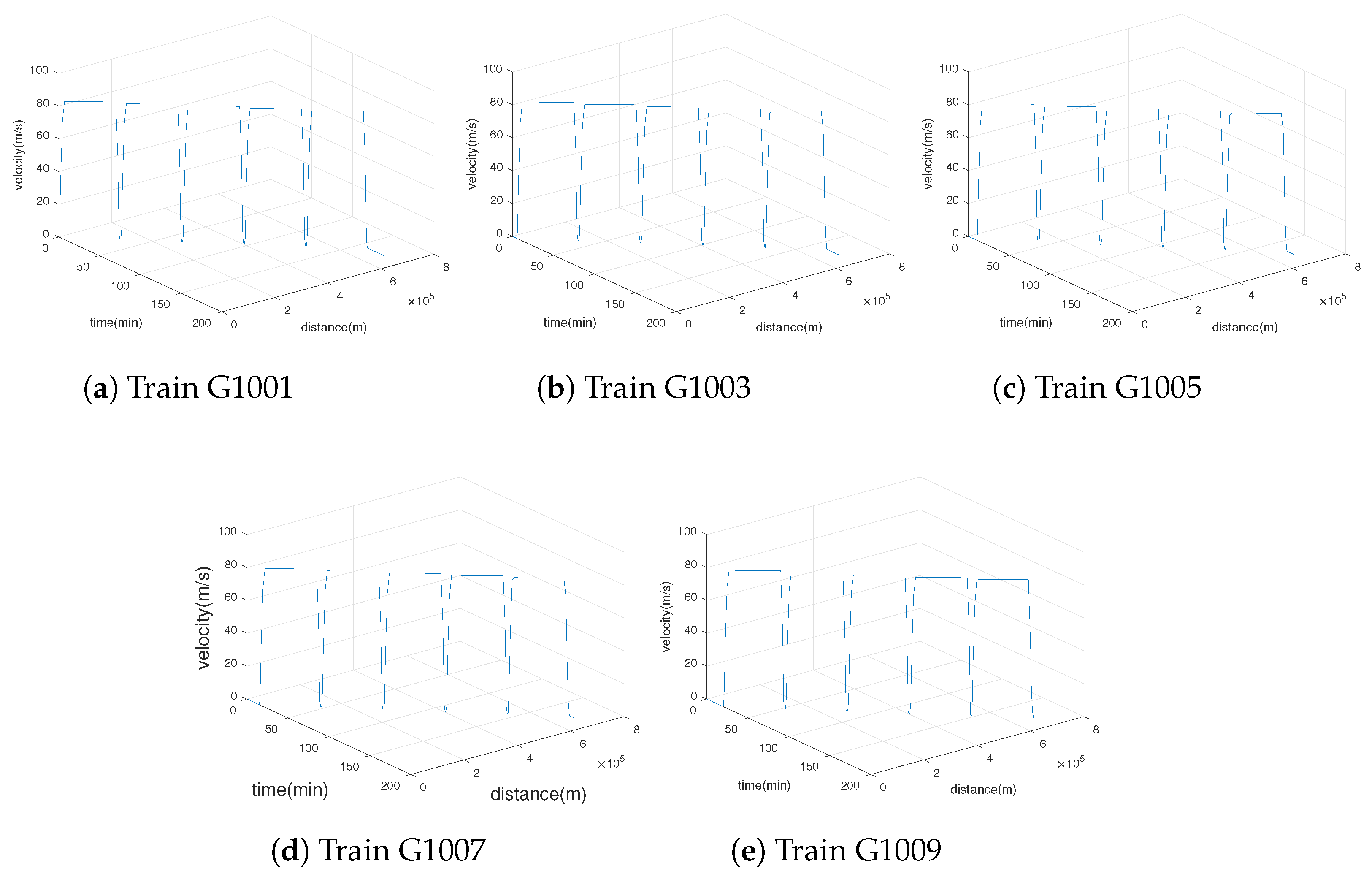
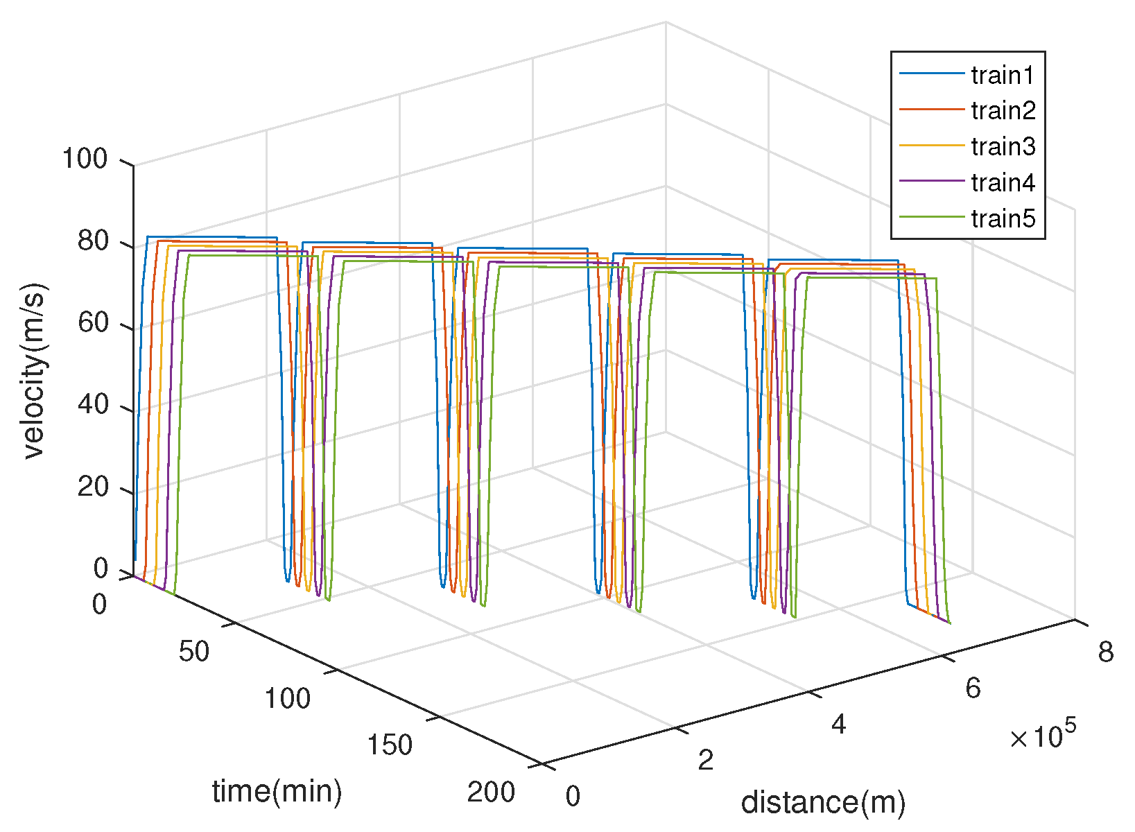
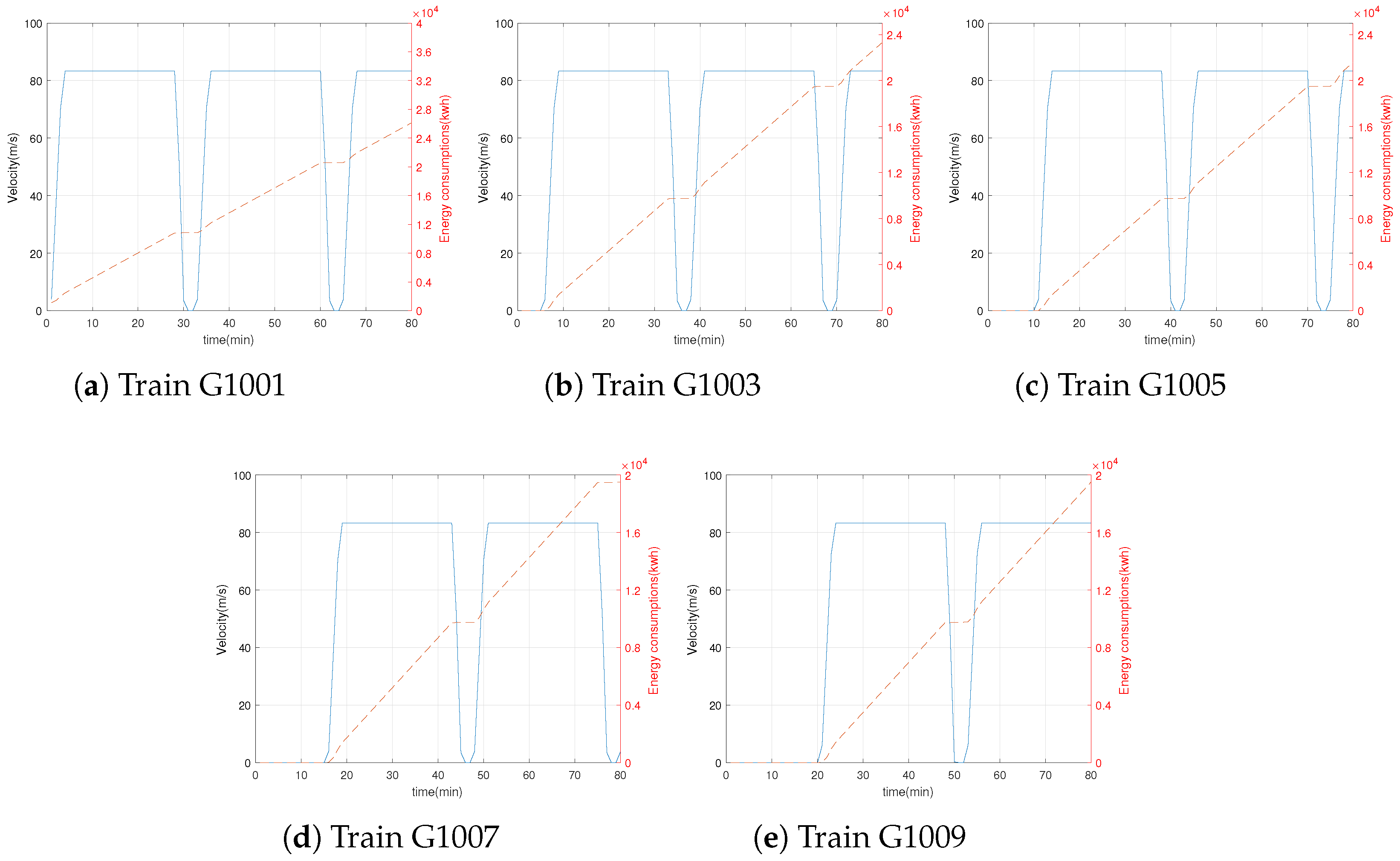
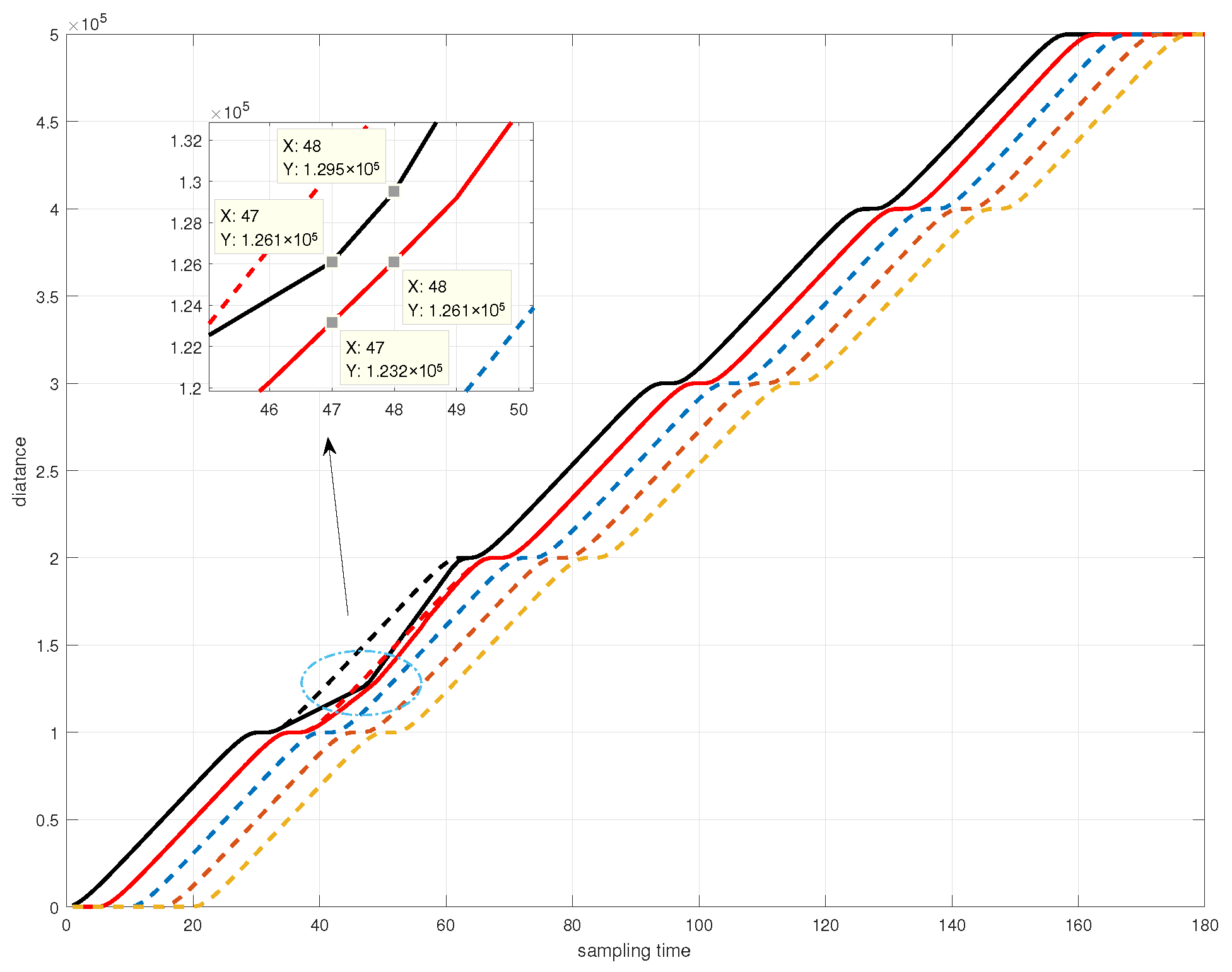
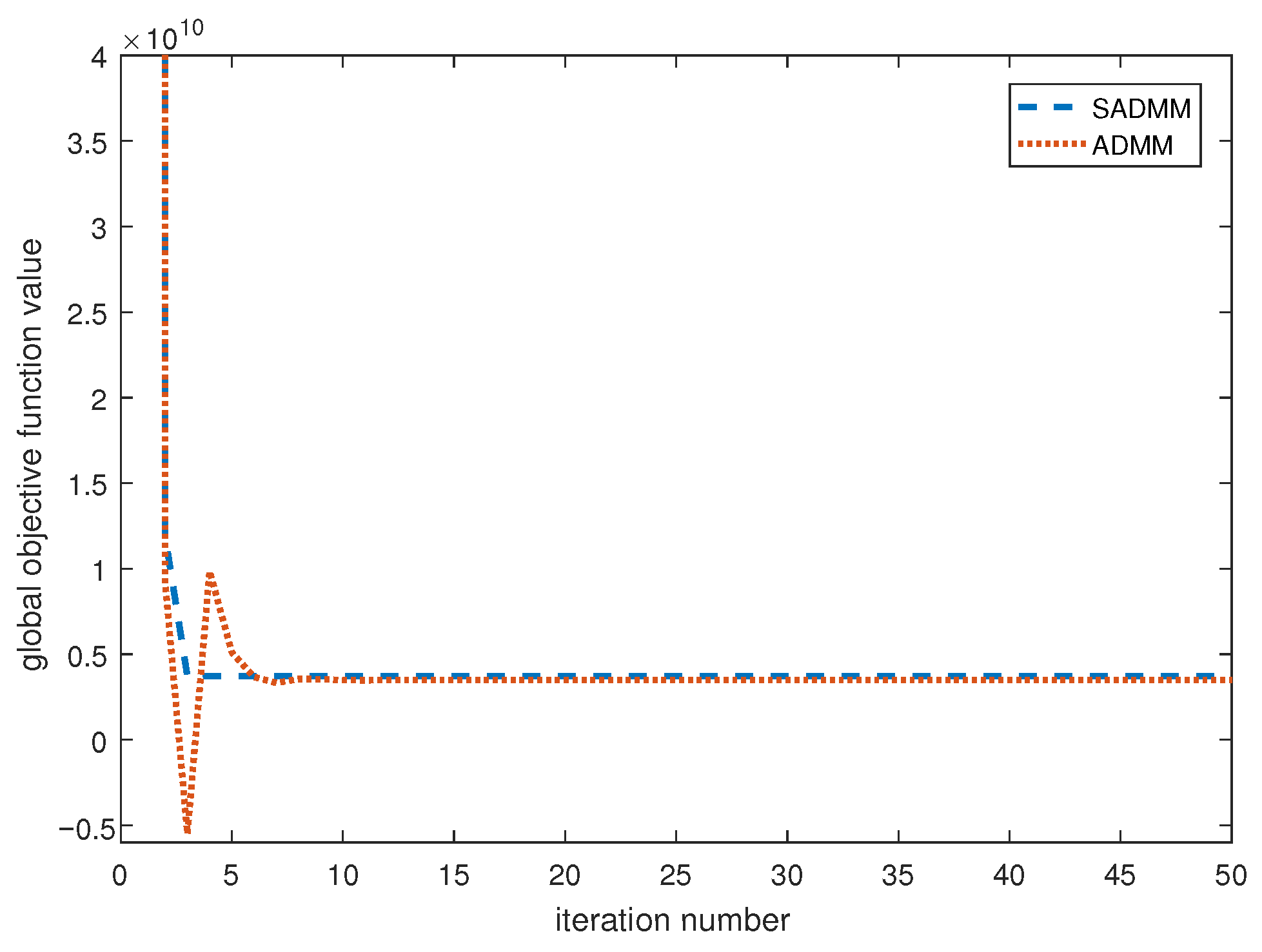
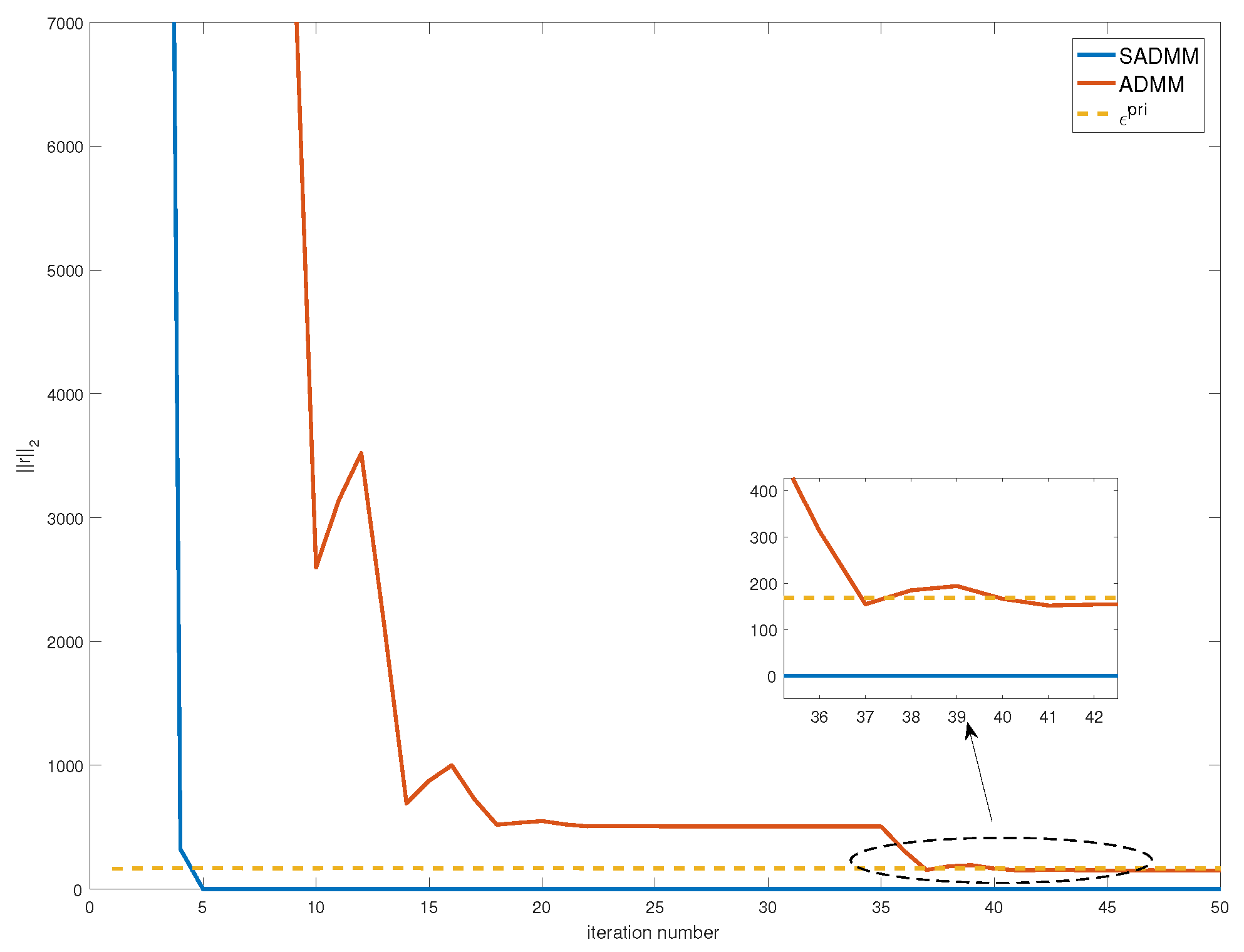
5. Numerical Simulations

In this section, we give a numerical experiment to illustrate the efficiency of our proposed algorithm. Our experiments are all executed on a computer with an Intel(R) Core (TM) i5-11300H processor (Intel Corporation, Santa Clara, CA, USA)CPU $3.10$ GHz and 16 GB memory. The source code is available from the GitHub repository on 14 May 2023 (https://github.com/ShanMa1/operation-control-of-trains.git).

The railway line in our experiment includes six stations and five trains. The speed limit of the trains is 300 km/h ($83.3$ m/s). The five trains are numbered G1001, G1003, G1005, G1007, and G1009. We assume that the distance between two adjacent stations is 135 km, the operation time of the trains between two adjacent stations is 30 min, and the headway buffer between two adjacent trains is 5 min. The planned timetable is shown in

Table 1. Scheduled timetable.

	Station	State	S1	S2	S3	S4	S5	S6
Train
G1001		arrive	8:00	8:28	8:58	9:28	9:58	10:28
		depart	8:00	8:30	9:00	9:30	10:00	10:30
G1003		arrive	-	8:33	9:03	9:33	10:03	10:33
		depart	8:05	8:35	9:05	9:35	10:05	10:35
G1005		arrive	-	8:38	9:08	9:38	10:08	10:38
		depart	8:10	8:40	9:10	9:40	10:10	10:40
G1007		arrive	-	8:43	9:13	9:43	9:13	10:43
		depart	8:15	8:45	9:15	9:45	10:15	10:45
G1009		arrive	-	8:48	9:18	9:48	10:18	10:48
		depart	8:20	8:50	9:20	9:50	10:20	10:50

and the train parameters are listed in

Table 2. Parameters of high-speed trains [18].

Parameters	Value	Unit
The weight of trains, $m_i,i=1,2,\dots ,5$	450	ton
Maximum acceleration, $a_{i,max}$	$0.56$	N/kg
Maximum deceleration, $a_{i,min}$	$0.8$	N/kg
Maximum control force, $F_{max}$	500	kN
Minimum control force, $F_{min}$	$-110$	kN
Resistance force, f	$-110$	kN
Sampled time period, d	60	s

. The weights $a_i$, $b_i$, and $q_i$ in the experiment are chosen as ${10}^7$, ${10}^7$, and 10, respectively. By using the proposed algorithm, our aim is to generate the optimal operation trajectories of trains while guaranteeing the safety and punctuality of trains.

By solving the optimal train operation control problem via SADMM, the optimal operation trajectory of each train can be obtained as shown in Figure 1. Figure 2 shows the optimal time-distance-speed profiles for 5 trains. Figure 3 shows the accumulated energy consumptions for the five trains under the optimal trajectory. In this figure, the blue lines denote the time-speed profiles, and the yellow lines denote the real-time energy consumption profiles.

Next, we consider the case that an emergency occurs, such that the first train receives a sudden speed limitation commend between stations $S2$ and $S3$. The speed of the first train is limited to 30 m/s. The duration of the emergency is assumed to be 15 min. By using our proposed algorithm, the optimal distance-time profile is obtained, as shown in Figure 4. In this figure, the dotted line represents the train operation profile without speed limitation, while the black line and red line denote the actual operation profile of the first train and the second train under the emergency, respectively. Since the speed of train $G1001$ is limited to 30 m/s, train $G1003$ has to slow down to keep a safe headway between train $G1001$. In this case, the minimum headway between train $G1001$ and train $G1003$ is 3 km. When the state of emergency is lifted, the speed of train $G1001$ will increase to achieve punctuality. In Figure 4, we can also find that the solution calculated by our proposed algorithm indicates that the trains could keep at least a minimum safe headway under the emergency.

Finally, we compare the computation effectiveness between SADMM and ADMM. The convergences of ADMM and SADMM are given as shown in Figure 5. Figure 6 shows the primal residual versus iterations. In this figure, we can see that SADMM can solve the optimal problem in 4 iterations, while ADMM can solve the optimal problem in 41 iterations. This means that SADMM converges faster than ADMM in our distributed control problem.

6. Conclusions

In this paper, for the dynamics of multiple trains with headway constraints and punctuality constraints, a distributed optimal control problem has been formulated to obtain the energy-efficient optimal train operation trajectories. The problem has been transformed into an optimization problem with several constraints. Then, we have proposed an efficient algorithm based on the framework of the symmetric alternating direction method of multipliers (SADMM) to solve this optimization problem. SADMM includes solving two convex optimization problems: the w-minimization problem and the z-minimization problem. The w-minimization problem could be solved by using the interior-point method, and the z-minimization problem could be solved via an analytical formula. Numerical simulations show that SADMM can obtain the optimal train control sequence in fewer iterative steps compared to the alternating direction multiplier method, thus illustrating the effectiveness of the algorithm. The results developed in this paper may have potential applications in the operational control of trains.

In particular, the results may find potential applications in future automatic train operation systems, where trains operate automatically and no driver is needed. In this case, the control inputs are generated according to algorithms, to ensure the punctuality and safety of trains.

References

1. Ichikawa, K. Application of optimization theory for bounded state variable problems to the operation of train. Bull. JSME 1968, 11, 857–865. [Google Scholar] [CrossRef]
2. Howlett, P. Optimal strategies for the control of a train. Automatica 1996, 32, 519–532. [Google Scholar] [CrossRef]
3. Guerra, T.-M.; Aguiar, B.; Berdjag, D.; Demaya, B. Robust estimation for nonlinear continuous-discrete systems with missing outputs: Application to automatic train control. IEEE Trans. Control. Syst. Technol. 2022, 30, 1304–1310. [Google Scholar] [CrossRef]
4. Havaei, P.; Sandidzadeh, M.A. Intelligent-PID controller design for speed track in automatic train operation system with heuristic algorithms. J. Rail Transp. Plan. Manag. 2022, 22, 100321. [Google Scholar] [CrossRef]
5. Ichikawa, S.; Miyatake, M. Energy efficient train trajectory in the railway system with moving block signaling scheme. IEEJ J. Ind. Appl. 2019, 8, 586–591. [Google Scholar] [CrossRef]
6. Sato, K.; Kato, H.; Fukushima, T. Development of SiC applied traction system for next-generation Shinkansen high-speed trains. IEEJ J. Ind. Appl. 2018, 9, 453–459. [Google Scholar] [CrossRef]
7. Nallaperuma, S.; Fletcher, D.; Harrison, R. Optimal control and energy storage for DC electric train systems using evolutionary algorithms. Railw. Eng. Sci. 2021, 29, 327–335. [Google Scholar] [CrossRef]
8. Khmelnitsky, E. On an optimal control problem of train operation. IEEE Trans. Autom. Control 2000, 45, 1257–1266. [Google Scholar] [CrossRef]
9. Bai, W.; Lin, Z.; Dong, H. Coordinated control in the presence of actuator saturation for multiple high-speed trains in the moving block signaling system mode. IEEE Trans. Veh. Technol. 2020, 69, 8054–8064. [Google Scholar] [CrossRef]
10. Li, S.; Yang, L.; Li, K.; Gao, Z. Robust sampled-data cruise control scheduling of high speed train. Transp. Res. Part C Emerg. Technol. 2014, 46, 274–283. [Google Scholar] [CrossRef]
11. Li, S.; Yang, L.; Gao, Z. Coordinated cruise control for high-speed train movements based on a multi-agent model. Transp. Res. Part C Emerg. Technol. 2015, 56, 281–292. [Google Scholar] [CrossRef]
12. Li, S.; Yang, L.; Li, K.; Gao, Z. Adaptive coordinated control of multiple high-speed trains with input saturation. Nonlinear Dyn. 2016, 83, 2157–2169. [Google Scholar] [CrossRef]
13. Lin, F.; Fardad, M.; Jovanovic, M.R. Optimal control of vehicular formations with nearest neighbor interactions. IEEE Trans. Autom. Control 2012, 57, 2203–2218. [Google Scholar] [CrossRef]
14. Yan, X.; Cai, B.; Ning, B.; ShangGuan, W. Online distributed cooperative model predictive control of energy-saving trajectory planning for multiple high-speed train movements. Transp. Res. Part C Emerg. Technol. 2016, 69, 60–78. [Google Scholar] [CrossRef]
15. Wang, Y.; De Schutter, B.; van den Boom, T.J.; Ning, B. Optimal trajectory planning for trains-a pseudospectral method and a mixed integer linear programming approach. Transp. Res. Part C Emerg. Technol. 2013, 29, 97–114. [Google Scholar] [CrossRef]
16. Boyd, S.; Parikh, N.; Eric, C.; Peleato, B.; Eckstein, J. Distributed optimization and statistical learning via the alternating direction method of multipliers. Found. Trends Mach. Learn. 2011, 3, 1–122. [Google Scholar] [CrossRef]
17. Lin, F.; Fardad, M.; Jovanović, M.R. Design of optimal sparse feedback gains via the alternating direction method of multipliers. IEEE Trans. Autom. Control 2013, 58, 2426–2431. [Google Scholar] [CrossRef]
18. Li, S.; Yang, L.; Gao, Z. Distributed optimal control for multiple high-speed train movement: An alternating direction method of multipliers. Automatica 2020, 112, 108646–108654. [Google Scholar] [CrossRef]
19. He, B.; Liu, H.; Wang, Z.; Yuan, X. A strictly contractive peaceman-rachford splitting method for convex programming. SIAM J. Optim. 2014, 24, 1011–1040. [Google Scholar] [CrossRef]
20. He, B.; Ma, F.; Yuan, X. Convergence study on the symmetric version of ADMM with larger step sizes. SIAM J. Imaging Sci. 2016, 9, 1467–1501. [Google Scholar] [CrossRef]
21. He, B.; Ma, F.; Yuan, X. Optimally linearizing the alternating direction method of multipliers for convex programming. Comput. Optim. Appl. 2020, 75, 361–388. [Google Scholar] [CrossRef]
22. Gao, B.; Ma, F. Symmetric alternating direction method with indefinite proximal regularization for linearly constrained convex optimization. J. Optim. Theory Appl. 2018, 176, 178–204. [Google Scholar] [CrossRef]
23. Jiao, Y.; Jin, Q.; Lu, X.; Wang, W. Alternating direction method of multipliers for linear inverse problems. SIAM J. Numer. Anal. 2016, 54, 2114–2137. [Google Scholar] [CrossRef]
24. Yang, L.; Luo, J.; Xu, Y.; Zhang, Z.; Dong, Z. A distributed dual consensus ADMM based on partition for dc-dopf with carbon emission trading. IEEE Trans. Ind. Inform. 2019, 16, 1858–1872. [Google Scholar] [CrossRef]
25. Nocedal, J.; Wright, S.J.; Mikosch, T.V.; Resnick, S.I.; Robinson, S.M. Numerical Optimization; Springer: Berlin/Heidelberg, Germany, 1999. [Google Scholar]
Figure 1. Optimal trajectory for five high-speed trains.
Axioms 12 00489 g001
Figure 2. The optimal time–distance–speed profiles for five high-speed trains.
Axioms 12 00489 g002
Figure 3. Energy consumption for five high-speed trains.
Axioms 12 00489 g003
Figure 4. Rescheduling solutions of first train and second train.
Axioms 12 00489 g004
Figure 5. Convergence curves of ADMM and SADMM.
Axioms 12 00489 g005
Figure 6. Primal residual versus iterations of ADMM and SADMM.
Axioms 12 00489 g006