Article

An Analytic Solution for 2D Heat Conduction Problems with General Dirichlet Boundary Conditions

1
Department of Aircraft Engineering, Air Force Institute of Technology, 1 Associate Jyulun Road, Gang-Shan District, Kaoshiung City 820, Taiwan
2
Department of Mechanical Engineering, Air Force Institute of Technology, 1 Associate Jyulun Road, Gang-Shan District, Kaoshiung City 820, Taiwan
*
Author to whom correspondence should be addressed.
Axioms 2023, 12(5), 416; https://doi.org/10.3390/axioms12050416
Submission received: 2 March 2023 / Revised: 8 April 2023 / Accepted: 20 April 2023 / Published: 24 April 2023
(This article belongs to the Special Issue Applied Mathematics in Energy and Mechanical Engineering)

Abstract

:
This paper proposed a closed-form solution for the 2D transient heat conduction in a rectangular cross-section of an infinite bar with the general Dirichlet boundary conditions. The boundary conditions at the four edges of the rectangular region are specified as the general case of space–time dependence. First, the physical system is decomposed into two one-dimensional subsystems, each of which can be solved by combining the proposed shifting function method with the eigenfunction expansion theorem. Therefore, through the superposition of the solutions of the two subsystems, the complete solution in the form of series can be obtained. Two numerical examples are used to investigate the analytic solution of the 2D heat conduction problems with space–time-dependent boundary conditions. The considered space–time-dependent functions are separable in the space–time domain for convenience. The space-dependent function is specified as a sine function and/or a parabolic function, and the time-dependent function is specified as an exponential function and/or a cosine function. In order to verify the correctness of the proposed method, the case of the space-dependent sinusoidal function and time-dependent exponential function is studied, and the consistency between the derived solution and the literature solution is verified. The parameter influence of the time-dependent function of the boundary conditions on the temperature variation is also investigated, and the time-dependent function includes harmonic type and exponential type.

1. Introduction

The application of heat conduction problems with time-dependent boundary conditions can be broadly applied in a wide range of engineering fields, such as time-varying heating on walls or plate panels, laser heating on solids, and the design of mechanical parts (such as those in turbines and engines [1,2]). In general, the types of time-dependent boundary conditions at the boundary surface include (1) the first type: specified temperature distribution (Dirichlet boundary condition); (2) the second type: specified heat flux distribution; and (3) the third type: convective heat exchange with the environment at a specified temperature. There are many methods to solve these three types of problems, such as pure numerical method, approximate method, and exact method. The literature review focuses on the study of 1D and 2D transient heat conduction problems with various time-dependent boundary conditions, as shown below.
For one-dimensional heat conduction problems with different kinds of time-dependent boundary conditions, these problems cannot be solved directly by the variable separation method due to the nonhomogeneity of boundary conditions. In the early 1970s, Ivanov and Salomatov [3,4] and Postol’Nik [5] were the first to transform the governing differential equation of the linear one-dimensional system into a nonlinear equation by introducing new variables. After neglecting the nonlinear terms, they obtained an approximated solution that they said was valid for the system with the Biot number less than 0.25. At the same time, Kozlov [6] used the Laplace transformation technique to study the problem with the Biot function in a rational combination of sine, cosine, polynomial and exponential functions. Although exact series solutions can be obtained for a given transformation system, great difficulties arise in the inversion of the transformation function, which is often not so straightforward. In addition, various approximation methods such as the iterative perturbation method [7], the eigenfunction expansion method [8], and the Lie point symmetry analysis method [9] have been used to study such heat conduction problems. Later in 2010, Lee and colleagues [10,11,12] proposed an integration-free solution method, which is an extension of the shifting function method developed in their previous research [13], to derive an analytic closed solution for the heat conduction with time-dependent boundary conditions of the second and the third types. Using the same method, they [14,15,16] had successfully performed one-dimensional inverse estimation of the heat treatment problem with unknown time-dependent boundary conditions of various types.
For the two-dimensional heat conduction problems with time-dependent boundary conditions, a considerable amount of work can be found in the literature on the development of exact, approximate, and numerical methods. In some advanced heat conduction books [17,18,19], some classical techniques such as Laplace transform, Duhamel’s theorem, and Green’s function have been proposed to solve them. Applying the Laplace transform starts with finding the solution of a 2D problem with nonhomogeneous boundary conditions in the transformed domain. Taking the inverse Laplace transform from the complex domain always has difficulties. The typical surveys included Zhu [20], Zhu et al. [21], and Sutradhar et al. [22] who dealt with the time derivative term in the diffusion equation by using the Laplace transform techniques. On the other hand, using Duhamel’s theorem [17], an auxiliary 2D problem with associated nonhomogeneous boundary conditions must first be solved. Therefore, the result will be obtained by differentiating under the integration. Similarly, Green’s function solution method [17] requires the derivation of the associated Green’s function, which satisfies a differential equation with a delta function and homogeneous boundary conditions. To obtain the general solution, the associated Green’s function must be directionally differentiated and integrated over the space and time domains. In addition, some numerical techniques, such as finite difference method and boundary element method, have also been used to solve 2D heat conduction problems with time-dependent boundary conditions. Bulgakov et al. [23] used the finite difference method to advance the solution in the time domain with the numerical schemes based on the boundary element method, while Walker [24] applied the diffusion fundamental solution combined with the time integration to solve the diffusion equation. Later, Chen et al. [25] applied the method of fundamental solutions for diffusion equations by using the modified Helmholtz fundamental solution. Burgess and Mahajerin [26] used the fundamental collocation method to solve the problems of arbitrary shapes subjected to arbitrary initial conditions and mixed time-dependent boundary conditions. The time-dependent fundamental solutions for diffusion equations were directly used by Young et al. [27] to obtain the solution as a linear combination of the fundamental solution of the diffusion operator. On the other hand, Cole and Yen [28] involved the method of Green’s function to obtain fast-converging expressions for the temperature and heat flux in a rectangular plate. Beck et al. [29] have developed the transient temperatures of the plates under time-varying heating conditions to an integer power at a surface. Lei et al. [30] presented a space–time generalized finite difference method (GFDM) to solve the transient heat conduction problem by integrating direct space–time discretization techniques into the meshless GFDM. Alam et al. [31] proposed a novel generalized (G’/G) extension technique for two nonlinear evolution equations: the (2+1) dimensional Konopelchenko–Dubrovsky (KD) equation and the (2+1) dimensional Kadomtsev–Petviashvili (KP) equations and obtained some new precise answers. The secured answers include a particular variety of solitary wave solutions. Islam et al. [32] applied a modified (G’/G) expansion method to seek new calculations of the Zakharov–Kuznetsov (ZK) equations developed in electrical engineering. Illustrated by 3D and contour plots, the mathematical results clearly demonstrate the complete honesty and high performance of the proposed algorithm. Krishnan et al. [33] proposed a technique based on eigenfunction expansion for solving 1D phase change heat transfer problems with time-dependent temperature or heat flux boundary conditions. By using Duhamel’s theorem, Belekar et al. [34] derived an analytic solution for the transient axisymmetric temperature distribution in a cylindrical geometry with time-dependent boundary conditions.
To the best of the authors’ knowledge, there is no literature formulating an analytic solution for the 2D heat conduction problems with the general Dirichlet boundary conditions specifying space–time-dependent dependent boundary conditions at the four edges of rectangular region. This paper develops a simplified exact solution method for the transient heat conduction in a rectangular cross-section of an infinite bar with space–time-dependent dependent boundary conditions using the shifting function method proposed by Lee and colleagues [10,11,12,13,14,15,16]. The study focuses on the 2D heat conduction problems with the general Dirichlet boundary conditions. For the two-dimensional problem, the original two-dimensional system is separated into two independent one-dimensional subsystems. The boundary conditions of the subsystems can then be changed from nonhomogeneous to homogeneous using the shifting function method, and an analytic solution can be derived using the eigenfunction expansion theorem. The solutions obtained from the two separate subsystems are combined to construct the solution of the original two-dimensional system. Finally, a numerical example is given, and the correctness of the obtained solution is verified via comparison with the literature [27]. Other case studies illustrate the feasibility of this approach.
The contributions of this paper are as follows:
(1)
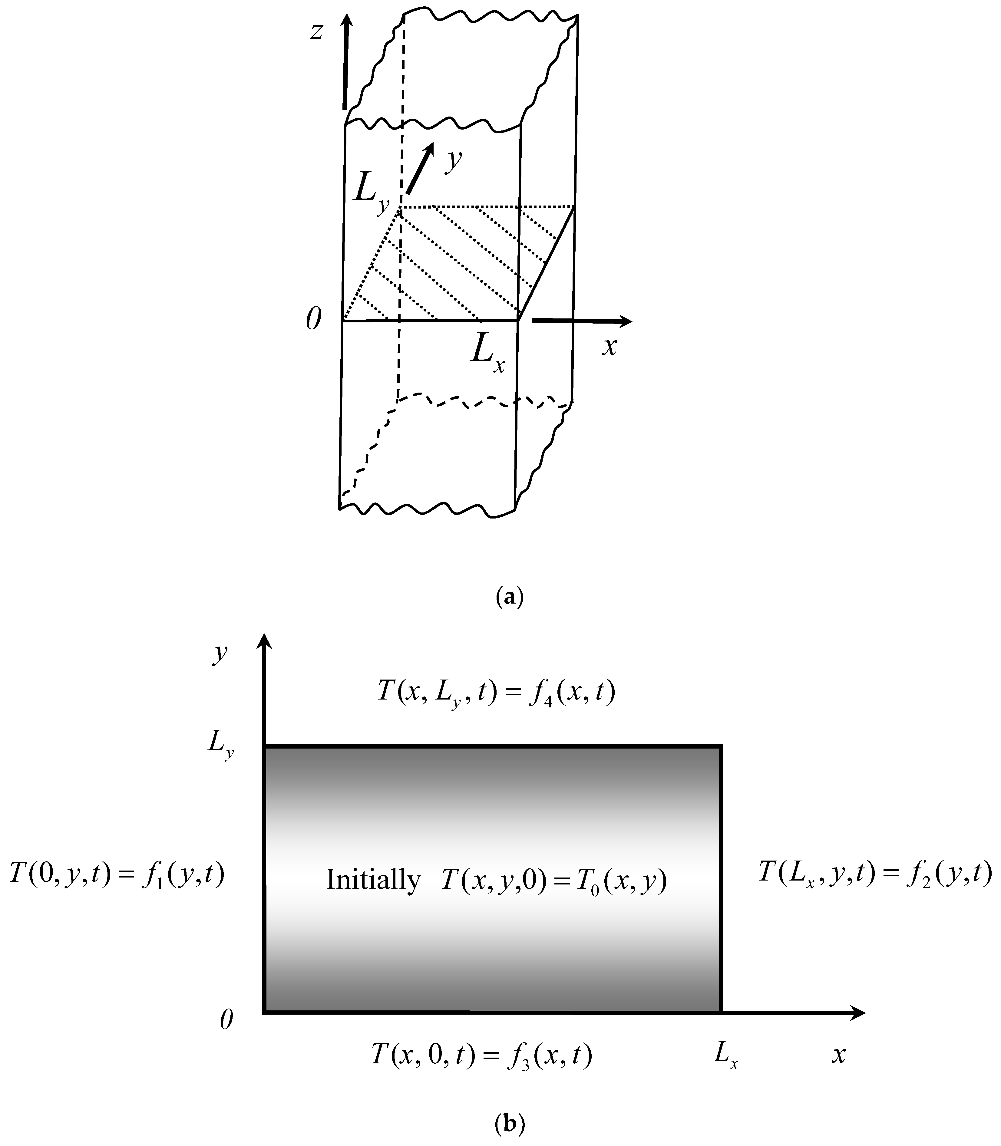
Lee and colleagues [10,11,12,13,14,15,16] used the shifting function method to derive an analytic solution for the heat conduction with time-dependent boundary conditions. They also performed an inverse estimation of a heat treatment problem with unknown time-dependent boundary conditions. However, their research is limited to the scope of one-dimensional heat conduction problems. The greatest contribution of this work is the first investigation of the analytic solution to 2D heat conduction problems with the general Dirichlet boundary conditions by using the proposed method, combining the shifting function method with the expansion theorem method. The applicability of the present method is in solving the heat conduction problems of a rectangular cross-section of an infinite rod with specified space–time-dependent dependent boundary conditions at the four edges of the rectangular region;
(2)
Some advanced heat conduction books [17,18,19] proposed some classical techniques such as the Laplace transform, Duhamel’s theorem, and Green’s function to solve the heat conduction problem. However, they are limited to the integration situation during the solution process. The correctness of the solution in this study is verified by comparing it with the results of Young et al. [27]. To the best of the authors’ knowledge, the other cases in this paper have never been presented in past studies. Although the number of series expansion terms determines the accuracy of the solution, the case study shows that the proposed method has good convergence to the solution using series expansion and can quickly reach a convergence value. The influence of the parameters of the time-dependent boundary function on the temperature variation is also studied.

2. Mathematical Modeling

Consider the transient heat conduction for a rectangular cross-section in an infinite bar with the space–time-dependent Dirichlet boundary conditions on its four sides and no heat generation in the medium. Figure 1 shows the geometry, the boundary conditions and initial condition of a rectangular cross-section in an infinite bar. The governing equation, boundary conditions and initial condition of the problem are as follows:
k [ 2 T ( x , y , t ) x 2 + 2 T ( x , y , t ) y 2 ] = ρ c T ( x , y , t ) t         in   0 < x < L x ,     0 < y < L y ,     t > 0 ,
T ( 0 , y , t ) = f 1 ( y , t )           at   x = 0 ,         0 y L y ,
T ( L x , y , t ) = f 2 ( y , t )           at   x = L x ,       0 y L y ,
T ( x , 0 , t ) = f 3 ( x , t )           at   y = 0 ,       0 x L x ,
T ( x , L y , t ) = f 4 ( x , t )           at   y = L y ,       0 x L x ,
T ( x , y , 0 ) = T 0 ( x , y )           at   t = 0 ,       0 x L x ,       0 y L y
where T ( x , y , t ) denotes the temperature function, x and y are the two-dimensional space variables, L x and L y are the thicknesses of the rectangular region at x and y directions, respectively, and t is the time variable. In addition, k is the thermal conductivity, ρ is the mass density, and c is the specific heat. It is noted that f i ( y , t ) i = 1 , 2 and f i ( x , t ) i = 3 , 4 denote the general case of space–time-dependent temperatures prescribed along the surfaces at the left and right ends and bottom and top ends, respectively. Furthermore, considering the matching of the boundary conditions with the initial conditions, one has
f 1 ( y , 0 ) = T 0 ( 0 , y ) ,       f 2 ( y , 0 ) = T 0 ( L x , y ) ,       f 3 ( x , 0 ) = T 0 ( x , 0 ) ,       f 4 ( x , 0 ) = T 0 ( x , L y ) .

3. The Solution Methodology

A dimensionless form of the 2D heat conduction system is first derived and split into two subsystems, each of which can be solved as a 1D problem. By properly introducing the shifting functions, the second-order governing differential equation with space–time-dependent boundary conditions are transformed into the differential equation with homogeneous boundary conditions.

3.1. The Dimensionless Form of Physical System

The dimensionless parameters are defined as follows:
θ ( X , Y , τ ) = T ( x , y , t ) T r ,   τ = α t L y 2 ,   X = x L x ,   Y = y L y ,   L r = L y L x ,       F 1 ( Y , τ ) = f 1 ( y , t ) T r ,
F 2 ( Y , τ ) = f 2 ( y , t ) T r ,   F 3 ( X , τ ) = f 3 ( x , t ) T r ,   F 4 ( X , τ ) = f 4 ( x , t ) T r ,   θ 0 ( X , Y ) = T 0 ( x , y ) T r .
The dimensionless form of the boundary-initial value problem is derived as follows:
[ L r 2 2 θ ( X , Y , τ ) X 2 + 2 θ ( X , Y , τ ) Y 2 ] = θ ( X , Y , τ ) τ       in   0 < X < 1 , 0 < Y < 1 ,   τ > 0 ,
θ ( 0 , Y , τ ) = F 1 ( Y , τ )           at   X = 0 ,           0 Y 1 ,
θ ( 1 , Y , τ ) = F 2 ( Y , τ )           at   X = 1 ,           0 Y 1 ,
θ ( X , 0 , τ ) = F 3 ( X , τ )           at   Y = 0 ,           0 X 1 ,
θ ( X , 1 , τ ) = F 4 ( X , τ )           at   Y = 1 ,           0 X 1 ,
θ ( X , Y , 0 ) = θ 0 ( X , Y )           at   τ = 0 ,           0 X 1 , 0 Y 1 ,
F 1 ( Y , 0 ) = θ 0 ( 0 , Y ) ,       F 2 ( Y , 0 ) = θ 0 ( 1 , Y ) ,       F 3 ( X , 0 ) = θ 0 ( X , 0 ) ,       F 4 ( X , 0 ) = θ 0 ( X , 1 )
where the parameter α = k ρ c in Equation (8) represents the thermal diffusivity and T r is the reference temperature.

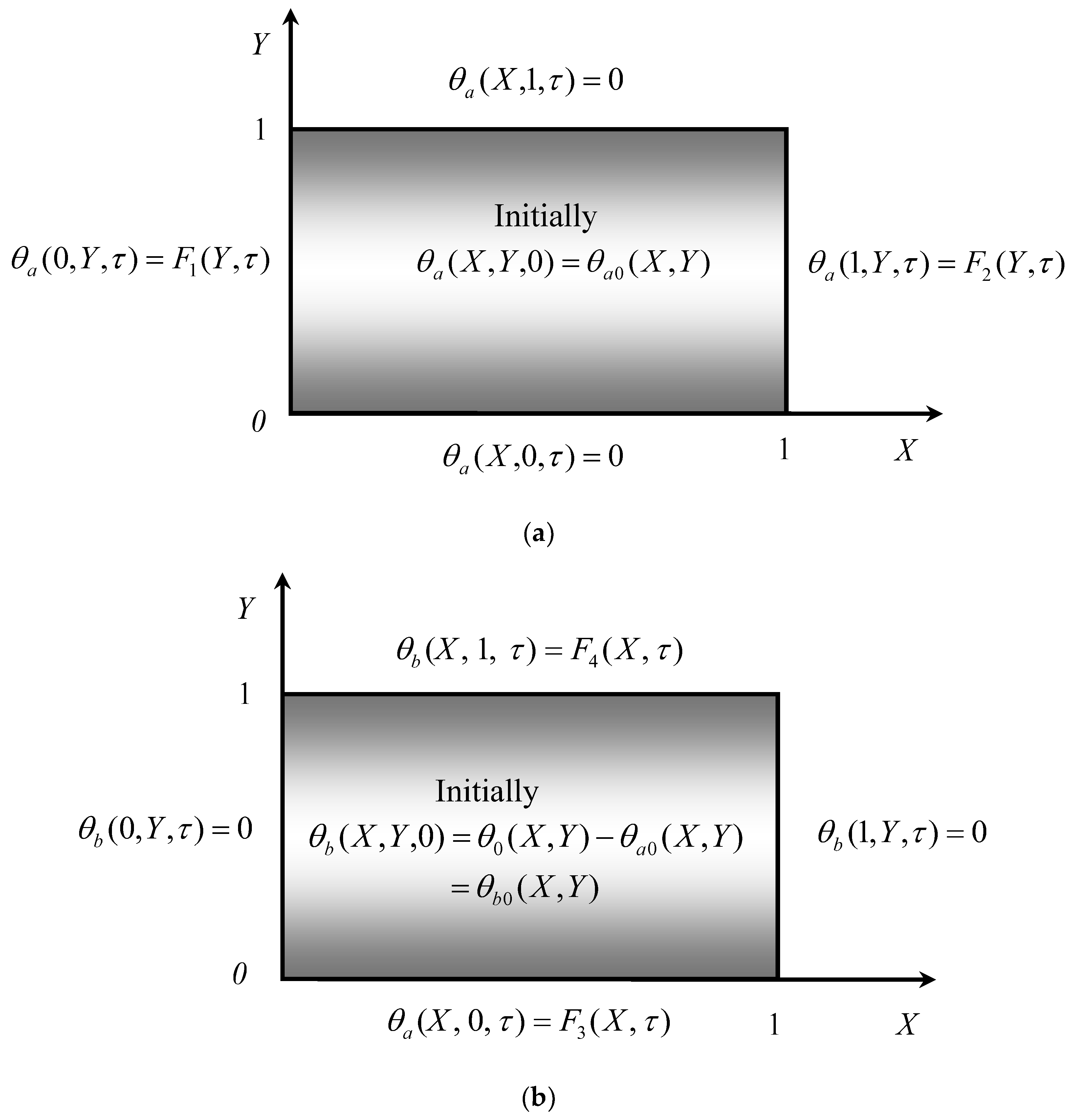
3.2. Principle of Superposition

Due to the linear property of the boundary value problem, the physical system can be divided into two subsystems, A and B along the X and Y directions by using the superposition principle, as shown in Figure 2; θ ( X , Y , τ ) is spilt into two parts as follows:
θ ( X , Y , τ ) = θ a ( X , Y , τ ) + θ b ( X , Y , τ ) .
For the subsystem A , the governing equation, boundary conditions and initial condition for the heat conduction problem are
[ L r 2 2 θ a ( X , Y , τ ) X 2 + 2 θ a ( X , Y , τ ) Y 2 ] = θ a ( X , Y , τ ) τ         in   0 < X < 1 , 0 < Y < 1 ,       τ > 0 ,
θ a ( 0 , Y , τ ) = F 1 ( Y , τ )           at   X = 0 ,           0 Y 1 ,
θ a ( 1 , Y , τ ) = F 2 ( Y , τ )           at   X = 1 ,           0 Y 1 ,
θ a ( X , 0 , τ ) = 0           at   Y = 0 ,           0 X 1 ,
θ a ( X , 1 , τ ) = 0           at   Y = 1 ,           0 X 1 ,
θ a ( X , Y , 0 ) = θ a 0 ( X , Y )           at   τ = 0 ,           0 X 1 , 0 Y 1 .
Likewise, for the subsystem B , the governing equation, boundary conditions and initial condition for the heat conduction problem are
[ L r 2 2 θ b ( X , Y , τ ) X 2 + 2 θ b ( X , Y , τ ) Y 2 ] = θ b ( X , Y , τ ) τ       in   0 < X < 1 , 0 < Y < 1 ,     τ > 0 ,
θ b ( 0 , Y , τ ) = 0           at   X = 0 ,           0 Y 1 ,
θ b ( 1 , Y , τ ) = 0           at   X = 1 ,           0 Y 1 ,
θ b ( X , 0 , τ ) = F 3 ( X , τ )           at   Y = 0 ,           0 X 1 ,
θ b ( X , 1 , τ ) = F 4 ( X , τ )           at   Y = 1 ,           0 X 1 ,
θ b ( X , Y , 0 ) = θ 0 ( X , Y ) θ a 0 ( X , Y ) = θ b 0 ( X , Y )           at   τ = 0 ,       0 X 1 , 0 Y 1 .
For the two similar subsystems, first solve the subsystem A , and then solve the subsystem B , listed in the Appendix A for brevity.

3.3. Reduced to One-Dimensional Problem

Considering the two homogeneous boundary conditions at the opposite edges of the rectangular region, namely, Y = 0 and Y = 1 , one can reasonably assume that the temperature θ a ( X , Y , τ ) and dimensionless quantities F i ( Y , τ ) ( i = 1 , 2 ) defined in Equations (18) and (19) are
θ a ( X , Y , τ ) = m = 1 [ θ m ( X , τ ) sin ( m π Y ) ] ,
F i ( Y , τ ) = m = 1 [ F ¯ i , m ( τ ) sin ( m π Y ) ] ,           ( i = 1 , 2 )
where F ¯ i , m ( τ ) ( i = 1 , 2 ) is defined as
F ¯ i , m ( τ ) = 2 0 1 F i ( Y , τ ) sin ( m π Y ) d Y , ( i = 1 , 2 ) .
Thus, θ m ( X , τ ) in Equation (29) is determined by satisfying the boundary conditions on both sides X = 0 and X = 1 (Equations (18) and (19)) and the governing equation. After substituting Equations (29) and (30) back into Equations (17)–(19), we can obtain the following results
θ m ( X , τ ) τ L r 2 2 θ m ( X , τ ) X 2 + m 2 π 2 θ m ( X , τ ) = 0           in   0 < X < 1 ,       τ > 0 ,
θ m ( 0 , τ ) = F ¯ 1 , m ( τ )           at   X = 0 ,
θ m ( 1 , τ ) = F ¯ 2 , m ( τ )           at   X = 1 ,
θ m ( X , 0 ) = 2 0 1 θ a 0 ( X , Y ) sin ( m π Y ) d Y           at   τ = 0 .

3.4. The Shifting Function Method

3.4.1. Change of Variable

To solve the second-order partial differential equation (Equation (32)) with nonhomogeneous boundary conditions (Equations (33) and (34)), the shifting function method developed by Lee and colleagues [10] is extended by employing the following transformation equation
θ m ( X , τ ) = θ ¯ m ( X , τ ) + i = 1 2 [ g i , m ( X ) F ¯ i , m ( τ ) ] .
where θ ¯ m ( X , τ ) is a transformed function and g i , m ( X ) ( i = 1 , 2 ) represents the two shift functions that need to be specified.
Substituting Equation (36) into Equations (32)–(34) can obtain
θ ¯ ˙ m ( X , τ ) + i = 1 2 [ g i , m ( X ) F ¯ ˙ i , m ( τ ) ] L r 2 { θ ¯ m ( X , τ ) + i = 1 2 [ g i , m ( X ) F ¯ i , m ( τ ) ] } + m 2 π 2 { θ ¯ m ( X , τ ) + i = 1 2 [ g i , m ( X ) F ¯ i , m ( τ ) ] } = 0
where the double primes are used to represent the twice differentiation with respect to X and the dots represent the differentiation with respect to τ , respectively.
The associated boundary conditions become
θ ¯ m ( 0 , τ ) + i = 1 2 [ g i , m ( 0 ) F ¯ i , m ( τ ) ] = F ¯ 1 , m ( τ ) ,
θ ¯ m ( 1 , τ ) + i = 1 2 [ g i , m ( 1 ) F ¯ i , m ( τ ) ] = F ¯ 2 , m ( τ ) .

3.4.2. The Shifting Functions

For the convenience of analysis, the shifting functions are specially selected so that they satisfy the following differential equations and boundary conditions
g i , m ( X ) = 0 , i = 1 , 2 ,           0 < X < 1 ,
g i , m ( 0 ) = δ i 1 ,             g i , m ( 1 ) = δ i 2
where δ i j is the Kronecker delta. Therefore, two shifting functions can be easily determined as
g 1 , m ( X ) = 1 X ,             g 2 , m ( X ) = X
After substituting Equations (40)–(42) back into Equations (37)–(39) yields a differential equation for θ ¯ m ( X , τ ) as below:
θ ¯ ˙ m ( X , τ ) L r 2 θ ¯ m ( X , τ ) + m 2 π 2 θ ¯ m ( X , τ ) = G ¯ m ( X , τ )
and the homogeneous boundary conditions become
θ ¯ m ( 0 , τ ) = 0 ,             θ ¯ m ( 1 , τ ) = 0
where G ¯ m ( X , τ ) in Equation (43) is defined as
G ¯ m ( X , τ ) = i = 1 2 { g i , m ( X ) [ F ¯ ˙ i , m ( τ ) + m 2 π 2 F ¯ i , m ( τ ) ] } .
Moreover, the initial condition can be transformed as
θ ¯ m ( X , 0 ) = 2 0 1 θ a 0 ( X , Y ) sin ( m π Y ) d Y i = 1 2 [ g i , m ( X ) F ¯ i , m ( 0 ) ] .

3.4.3. The Eigenfunction Expansion Theorem

The solution θ ¯ m ( X , τ ) specified by Equations (43) and (44) can be expressed by applying the method of separation variable as
θ ¯ m ( X , τ ) = n = 1 [ θ ¯ m n ( X ) T m n a ( τ ) ]
where the space variable θ ¯ m n ( X ) satisfies the following Sturm–Liouville eigenvalue problem
θ ¯ m n ( X ) + ω n 2 θ ¯ m n ( X ) = 0 ,             0 < X < 1 ,
θ ¯ m n ( 0 ) = 0             at       X = 0 ,
θ ¯ m n ( 1 ) = 0             at       X = 1 .
It is noted that the eigenfunctions θ ¯ m n ( X ) ( n = 1 , 2 , 3 , ) and the corresponding eigenvalues are
θ ¯ m n ( X ) = sin ω n X ,         ω n = n π ,         ( n = 1 , 2 , 3 , )
In addition, the eigenfunctions form an orthogonal set in the interval [ 0 , 1 ] as
0 1 θ ¯ m i ( X ) θ ¯ m j ( X ) d X = { 0 for i j , 1 2 for i = j .
Substituting Equation (47) into Equation (43), multiplying it by θ ¯ m n ( X ) , and integrating from 0 to 1, one will obtain the following differential equation
T ˙ m n a ( τ ) + λ m n a 2 T m n a ( τ ) = γ m n a ( τ )
where λ m n a and γ m n a ( τ ) are given as
λ m n a = m 2 + n 2 L r 2 π ,
γ m n a ( τ ) = 2 0 1 θ ¯ m n ( X ) G ¯ m ( X , τ ) d X = 2 n π { [ F ¯ ˙ 1 , m ( τ ) ( 1 ) n F ¯ ˙ 2 , m ( τ ) ] + m 2 π 2 [ F ¯ 1 , m ( τ ) ( 1 ) n F ¯ 2 , m ( τ ) ] } .
T m n a ( 0 ) is determined from the initial condition of the transformed function defined in Equation (46) as
T m n a ( 0 ) = 2 0 1 θ ¯ m n ( X ) θ ¯ m ( X , 0 ) d X = 4 0 1 sin ( n π X ) 0 1 θ a 0 ( X , Y ) sin ( m π Y ) d Y d X 2 n π [ F ¯ 1 , m ( 0 ) ( 1 ) n F ¯ 2 , m ( 0 ) ] .
Therefore, the general solution to Equation (53) with the above initial conditions is
T m n a ( τ ) = e λ m n a 2 τ T m n a ( 0 ) + 0 τ e λ m n a 2 ( τ ϕ ) γ m n a ( ϕ ) d ϕ .

3.5. The Analytic Solution

After substituting the solution of the transformed function in Equation (47), and the shifting functions in Equation (42), back into Equations (36) and (29), we can derive the closed-form solution for the θ a ( X , Y , τ ) subsystem as follows:
θ a ( X , Y , τ ) = m = 1 { n = 1 [ sin ( n π X ) T m n a ( τ ) ] + ( 1 X ) F ¯ 1 , m ( τ ) + X F ¯ 2 , m ( τ ) } sin ( m π Y ) .
Due to the high symmetry with the θ a ( X , Y , τ ) subsystem, the solution form of the θ b ( X , Y , τ ) subsystem can be easily obtained through a similar derivation process (see Appendix A for details) as
θ b ( X , Y , τ ) = m = 1 { n = 1 [ sin ( n π Y ) T m n b ( τ ) ] + ( 1 Y ) F ¯ 3 , m ( τ ) + Y F ¯ 4 , m ( τ ) } sin ( m π X ) .
Finally, adding the solutions of the two subsystems, the analytic solution for the 2D heat conduction in a rectangular region with the general Dirichlet boundary conditions is obtained as follows:
θ ( X , Y , τ ) = m = 1 { n = 1 [ sin ( n π X ) T m n a ( τ ) ] + ( 1 X ) F ¯ 1 , m ( τ ) + X F ¯ 2 , m ( τ ) } sin ( m π Y ) + m = 1 { n = 1 [ sin ( n π Y ) T m n b ( τ ) ] + ( 1 Y ) F ¯ 3 , m ( τ ) + Y F ¯ 4 , m ( τ ) } sin ( m π X ) .
From the above derivation process, it can be seen that the assumptions in Equations (29) and (A5) have restrictions on the boundary conditions and initial condition; that is, these values at the four corners of the rectangular region should be zero. If the values of the boundary conditions and initial condition at the four corners of the rectangular region are not zero, they should be zeroed first.

4. Examples and Verification

To illustrate the advantages of the proposed method, two examples with different types of space-dependent boundary conditions are examined in detail below:

4.1. The Space-Dependent Boundary Conditions of Periodical Type

Example 1: 
Consider a linear 2D heat conduction problem in a rectangular region ( L x = L y = L r = 1 ) subject to the space–time-dependent boundary conditions and initial condition as follows:
T ( 0 , y , t ) = f 1 ( y , t ) = [ sin ( π y ) ] η 1 ( α t )           at   x = 0 ,       0 y 1 ,
T ( 1 , y , t ) = f 2 ( y , t ) = [ sin ( π y ) ] η 2 ( α t )           at   x = 1 ,       0 y 1 ,
T ( x , 0 , t ) = f 3 ( x , t ) = [ sin ( π x ) ] η 3 ( α t )           at   y = 0 ,       0 x 1 ,
T ( x , 1 , t ) = f 4 ( x , t ) = [ sin ( π x ) ] η 4 ( α t )           at   y = 1 ,       0 x 1 ,
T ( x , y , 0 ) = sin π x + sin π y           at   t = 0 ,       0 x 1 ,       0 y 1 .
Following the present solution procedure and using the dimensionless parameters defined in Equation (8), we can change the space–time-dependent boundary and initial conditions to
θ ( 0 , Y , τ ) = F 1 ( Y , τ ) = sin ( π Y ) T r η 1 ( τ )           at   X = 0 ,       0 Y 1 ,
θ ( 1 , Y , τ ) = F 2 ( Y , τ ) = sin ( π Y ) T r η 2 ( τ )           at   X = 1 ,       0 Y 1 ,
θ ( X , 0 , τ ) = F 3 ( X , τ ) = sin ( π X ) T r η 3 ( τ )           at   Y = 0 ,       0 X 1 ,
θ ( X , 1 , τ ) = F 4 ( X , τ ) = sin ( π X ) T r η 4 ( τ )           at   Y = 1 ,       0 X 1 ,
θ ( X , Y , 0 ) = [ sin ( π X ) + sin ( π Y ) ] T r           at   τ = 0 ,       0 X 1 ,       0 Y 1 .
The temperature θ ( X , Y , 0 ) is divided into two parts as follows:
θ a 0 ( X , Y , 0 ) = sin ( π Y ) T r ,             θ b 0 ( X , Y , 0 ) = sin ( π X ) T r .
In this case, using one-term expansion ( m = n = 1 ) in the analytic solution derived from Equation (60), the solution is derived as
θ ( X , Y , τ ) = [ sin ( π X ) T 11 a ( τ ) + ( 1 X ) F ¯ 1 , 1 ( τ ) + X F ¯ 2 , 1 ( τ ) ] sin ( π Y ) + [ sin ( π Y ) T 11 b ( τ ) + ( 1 Y ) F ¯ 3 , 1 ( τ ) + Y F ¯ 4 , 1 ( τ ) ] sin ( π X )
where the associated dimensionless quantity F ¯ i , 1 ( τ ) ( i = 1 , 2 , 3 , 4 ) is
F ¯ i , 1 ( τ ) = η i ( τ ) T r , i = 1 , 2 , 3 , 4
T 11 a ( 0 ) and T 11 b ( 0 ) are determined from the initial conditions of the transformed functions defined in Equations (46) and (A25) as
T 11 a ( 0 ) = 4 π 2 π [ η 1 ( 0 ) + η 2 ( 0 ) ] ,           T 11 b ( 0 ) = 4 π 2 π [ η 3 ( 0 ) + η 4 ( 0 ) ]
Likewise, from Equations (54) and (55), and Equations (A23) and (A24), one obtains
λ 11 a = λ 11 b = 2 π ,
γ 11 a ( τ ) = 2 π { η ˙ 1 ( τ ) + η ˙ 2 ( τ ) + π 2 [ η 1 ( τ ) + η 2 ( τ ) ] } , γ 11 b ( τ ) = 2 π { η ˙ 3 ( τ ) + η ˙ 4 ( τ ) + π 2 [ η 3 ( τ ) + η 4 ( τ ) ] } ,
Therefore, one can obtain
T 11 a ( τ ) = 4 π e 2 π 2 τ 2 π [ η 1 ( τ ) + η 2 ( τ ) ] + 2 π 0 τ e 2 π 2 ( τ ϕ ) [ η 1 ( ϕ ) + η 2 ( ϕ ) ] d ϕ ,
T 11 b ( τ ) = 4 π e 2 π 2 τ 2 π [ η 3 ( τ ) + η 4 ( τ ) ] + 2 π 0 τ e 2 π 2 ( τ ϕ ) [ η 3 ( ϕ ) + η 4 ( ϕ ) ] d ϕ .
(Case 1): Consider the time-dependent functions to be of exponential type, as follows:
η i ( τ ) = e π 2 τ ,           ( i = 1 , 2 , 3 , 4 ) .
From Equations (77) and (78) one obtains
T 11 a ( τ ) = T 11 b ( τ ) = 0 .
The solution from the dimensionless form of Equation (72) becomes
θ ( X , Y , τ ) = [ sin ( π X ) + sin ( π Y ) ] e π 2 τ T r .
Substituting this back into dimensional form would be
T ( x , y , t ) = [ sin ( π x ) + sin ( π y ) ] e α π 2 t .
It can be seen that the solution obtained in Equation (82) is exactly the same form as that given by Young et al. [25].
(Case 2): Consider the time-dependent functions to be of periodic type, as follows:
η i ( τ ) = cos ( ω i τ ) ,           ( i = 1 , 2 , 3 , 4 ) .
One obtains
γ 11 a ( τ ) = 2 π [ ω 1 sin ( ω 1 τ ) ω 2 sin ( ω 2 τ ) + π 2 cos ( ω 1 τ ) + π 2 cos ( ω 2 τ ) ] ,
γ 11 b ( τ ) = 2 π [ ω 3 sin ( ω 3 τ ) ω 4 sin ( ω 4 τ ) + π 2 cos ( ω 3 τ ) + π 2 cos ( ω 4 τ ) ]
T 11 a ( τ ) = 2 π e 2 π 2 τ ( 2 π 4 + ω 1 2 4 π 4 + ω 1 2 + 2 π 4 + ω 2 2 4 π 4 + ω 2 2 ) 2 π [ ( 2 π 4 + ω 1 2 ) cos ( ω 1 π ) π 2 ω 1 sin ( ω 1 π ) 4 π 4 + ω 1 2 + ( 2 π 4 + ω 2 2 ) cos ( ω 2 π ) π 2 ω 2 sin ( ω 2 π ) 4 π 4 + ω 2 2 ] ,
T 11 b ( τ ) = 2 π e 2 π 2 τ ( 2 π 4 + ω 3 2 4 π 4 + ω 3 2 + 2 π 4 + ω 4 2 4 π 4 + ω 4 2 ) 2 π [ ( 2 π 4 + ω 3 2 ) cos ( ω 3 π ) π 2 ω 3 sin ( ω 3 π ) 4 π 4 + ω 3 2 + ( 2 π 4 + ω 4 2 ) cos ( ω 4 π ) π 2 ω 4 sin ( ω 4 π ) 4 π 4 + ω 4 2 ] .
Therefore, the exact solution in dimensionless form becomes
θ ( X , Y , τ ) = [ sin ( π X ) T 11 a ( τ ) + ( 1 X ) cos ( ω 1 τ ) T r + X cos ( ω 2 τ ) T r ] sin ( π Y ) + [ sin ( π Y ) T 11 b ( τ ) + ( 1 Y ) cos ( ω 3 τ ) T r + Y cos ( ω 4 τ ) T r ] sin ( π X ) .
Three cases including ω i = π ( i = 1 , 2 , 3 , 4 ) , ω i = 5 ( i = 1 , 2 , 3 , 4 ) , and ω i = 7 ( i = 1 , 2 , 3 , 4 ) will be considered in the numerical analysis. Figure 3 illustrates the temperature-time variation in the middle of a rectangular region with various parameter values of ω i ( i = 1 , 2 , 3 , 4 ) , which shows the oscillating behavior, as expected. In addition, the larger the parameter value of ω i ( i = 1 , 2 , 3 , 4 ) , the more frequent the temperature fluctuation.

4.2. The Space-Dependent Boundary Conditions of Parabolic Type

Example 2: 
Consider a 2D transient heat conduction problem in a rectangular region ( L x = L y = L r = 1 ).
The boundary and initial conditions are listed as follows:
T ( 0 , y , t ) = f 1 ( y , t ) = ( y y 2 ) η 1 ( α t )           at   x = 0 ,       0 y 1 ,
T ( 1 , y , t ) = f 2 ( y , t ) = ( y y 2 ) η 2 ( α t )           at   x = 1 ,       0 y 1 ,
T ( x , 0 , t ) = f 3 ( x , t ) = ( x x 2 ) η 3 ( α t )           at   y = 0 ,       0 x 1 ,
T ( x , 1 , t ) = f 4 ( x , t ) = ( x x 2 ) η 4 ( α t )           at   y = 1 ,       0 x 1 ,
T ( x , y , 0 ) = ( x x 2 ) + ( y y 2 )           at   t = 0 ,       0 x 1 ,       0 y 1
Using the dimensionless parameters generates
θ ( 0 , Y , τ ) = Y Y 2 T r η 1 ( τ ) F 1 ( Y , τ )           at   X = 0 ,       0 Y 1 ,
θ ( 1 , Y , τ ) = Y Y 2 T r η 2 ( τ ) F 2 ( Y , τ )           at   X = 1 ,       0 Y 1 ,
θ ( X , 0 , τ ) = X X 2 T r η 3 ( τ ) F 3 ( X , τ )           at   Y = 0 ,       0 X 1 ,
θ ( X , 1 , τ ) = X X 2 T r η 4 ( τ ) F 4 ( X , τ )           at   Y = 0 ,       0 X 1 ,
θ ( X , Y , 0 ) = ( X X 2 ) + ( Y Y 2 ) T r           at   τ = 0 ,       0 X 1 ,       0 Y 1 ,
and separating θ ( X , Y , 0 ) into two parts yields
θ a 0 ( X , Y , 0 ) = Y Y 2 T r ,             θ b 0 ( X , Y , 0 ) = X X 2 T r .
Following the same solution procedure, the associated dimensionless quantity F ¯ i , m ( τ ) ( i = 1 , 2 , 3 , 4 ) becomes
F ¯ i , m ( τ ) = 4 [ 1 ( 1 ) m ] m 3 π 3 T r η i ( τ ) , i = 1 , 2 , 3 , 4 .
To determine T m n a ( τ ) and T m n b ( τ ) , one derives first
λ m n a = λ m n b = m 2 + n 2 π ,
T m n a ( 0 ) = 8 [ 1 ( 1 ) m ] m 3 n π 4 T r [ 1 ( 1 ) n η 1 ( 0 ) + ( 1 ) n η 2 ( 0 ) ] ,
T m n b ( 0 ) = 8 [ 1 ( 1 ) m ] m 3 n π 4 T r [ 1 ( 1 ) n η 3 ( 0 ) + ( 1 ) n η 4 ( 0 ) ] ,
γ m n a ( τ ) = 8 [ 1 ( 1 ) m ] m 3 n π 4 T r { η ˙ 1 ( τ ) ( 1 ) n η ˙ 2 ( τ ) + m 2 π 2 [ η 1 ( τ ) ( 1 ) n η 2 ( τ ) ] } ,
γ m n b ( τ ) = 8 [ 1 ( 1 ) m ] m 3 n π 4 T r { η ˙ 3 ( τ ) ( 1 ) n η ˙ 4 ( τ ) + m 2 π 2 [ η 3 ( τ ) ( 1 ) n η 4 ( τ ) ] } .
Accordingly, the solutions for T m n a ( τ ) and T m n b ( τ ) are
T m n a ( τ ) = 8 [ 1 ( 1 ) m ] m 3 n π 4 T r { [ 1 ( 1 ) n ] e λ m n a 2 τ η 1 ( τ ) + ( 1 ) n η 2 ( τ ) ] + n 2 π 2 0 τ e λ m n a 2 ( τ ϕ ) [ η 1 ( ϕ ) ( 1 ) n η 2 ( ϕ ) ] d ϕ } ,
T m n b ( τ ) = 8 [ 1 ( 1 ) m ] m 3 n π 4 T r { [ 1 ( 1 ) n ] e λ m n b 2 τ η 3 ( τ ) + ( 1 ) n η 4 ( τ ) ] + n 2 π 2 0 τ e λ m n b 2 ( τ ϕ ) [ η 3 ( ϕ ) ( 1 ) n η 4 ( ϕ ) ] d ϕ } .
Therefore, the exact solution in dimensionless form is
θ ( X , Y , τ ) = m = 1 { n = 1 [ sin ( n π X ) T m n a ( τ ) ] + 4 ( 1 X ) [ 1 ( 1 ) m ] m 3 π 3 T r η 1 ( τ ) + 4 X [ 1 ( 1 ) m ] m 3 π 3 T r η 2 ( τ ) } sin ( m π Y ) + m = 1 { n = 1 [ sin ( n π Y ) T m n b ( τ ) ] + 4 ( 1 Y ) [ 1 ( 1 ) m ] m 3 π 3 T r η 3 ( τ ) + 4 Y [ 1 ( 1 ) m ] m 3 π 3 T r η 4 ( τ ) } sin ( m π X ) .
Considering the time-dependent term of exponential type as
η i ( τ ) = e d i τ ,             ( i = 1 , 2 , 3 , 4 ) ,
one has
T m n a ( τ ) = 8 [ 1 ( 1 ) m ] m 3 n π 4 T r { [ 1 ( 1 ) n ] e λ m n a 2 τ e d 1 τ + ( 1 ) n e d 2 τ ] + n 2 π 2 [ e d 1 τ e λ m n a 2 τ λ m n a 2 d 1 ( 1 ) n e d 2 τ e λ m n a 2 τ λ m n a 2 d 2 ] } ,
T m n b ( τ ) = 8 [ 1 ( 1 ) m ] m 3 n π 4 T r { [ 1 ( 1 ) n ] e λ m n b 2 τ e d 3 τ + ( 1 ) n e d 4 τ ] + n 2 π 2 [ e d 3 τ e λ m n b 2 τ λ m n b 2 d 3 ( 1 ) n e d 4 τ e λ m n b 2 τ λ m n b 2 d 4 ] }
where d i ( i = 1 , 2 , 3 , 4 ) .represents four arbitrary constants. Table 1, Table 2 and Table 3 shows the temperature variation of the midpoint of the rectangular region under the three kinds of exponential parameters of d i ( i = 1 , 2 , 3 , 4 ) . It can be found that the solutions developed converge to convergence values as the number of series terms ( m = n ) increases. The temperature at 0 τ 1.2 are the same between 10 and 20 terms expansion. The results converge when 10 terms expansion is used. By comparing the temperature at 0 τ 1.2 between 5 and 10 terms expansion in each table of Table 1, Table 2 and Table 3, one can see that when 5 terms expansion is used, the error of the solution evaluated is less than 1%. Therefore, 5 terms expansion ( m = n ) of the series will be taken for the numerical analysis below. Figure 4 illustrates the temperature variation in the middle of the rectangular region with respect to time τ for three different kinds of di (i = 1, 2, 3, 4). It is seen from Figure 4 that the temperature curve of the set of d i = 1 ( i = 1 , 2 , 3 , 4 ) decays faster than the other two curves, and the trend of the temperature curves of three sets is the same.

5. Conclusions

A closed form solution of the transient heat conduction in a rectangular cross-section in an infinite bar with the general space–time-dependent boundary conditions has been developed in terms of series expansion. The main advantages of the proposed solution method is that differentiation and/or integration of the Green’s function is not required and the solution of the auxiliary 2D problem with associated nonhomogeneous boundary conditions is avoided. Two examples are given to illustrate the applicability of the method and the example of space-dependent boundary for periodic function is shown to be consistent with results in the literature.
The new findings of the present study are as follows:
(1)
The proposed approach combining the shifting function method and the expansion theorem method can derive an analytic solution for the 2D heat conduction in a rectangular cross-section of an infinite bar with the general Dirichlet boundary conditions specifying space–time-dependent boundary conditions at the four edges of the rectangular region;
(2)
The series expansion derived from the proposed method has a good convergence to reach the convergence values. For space-dependent boundary with the parabolic-type case, one can take five terms of the series to obtain the series solutions within 1% error;
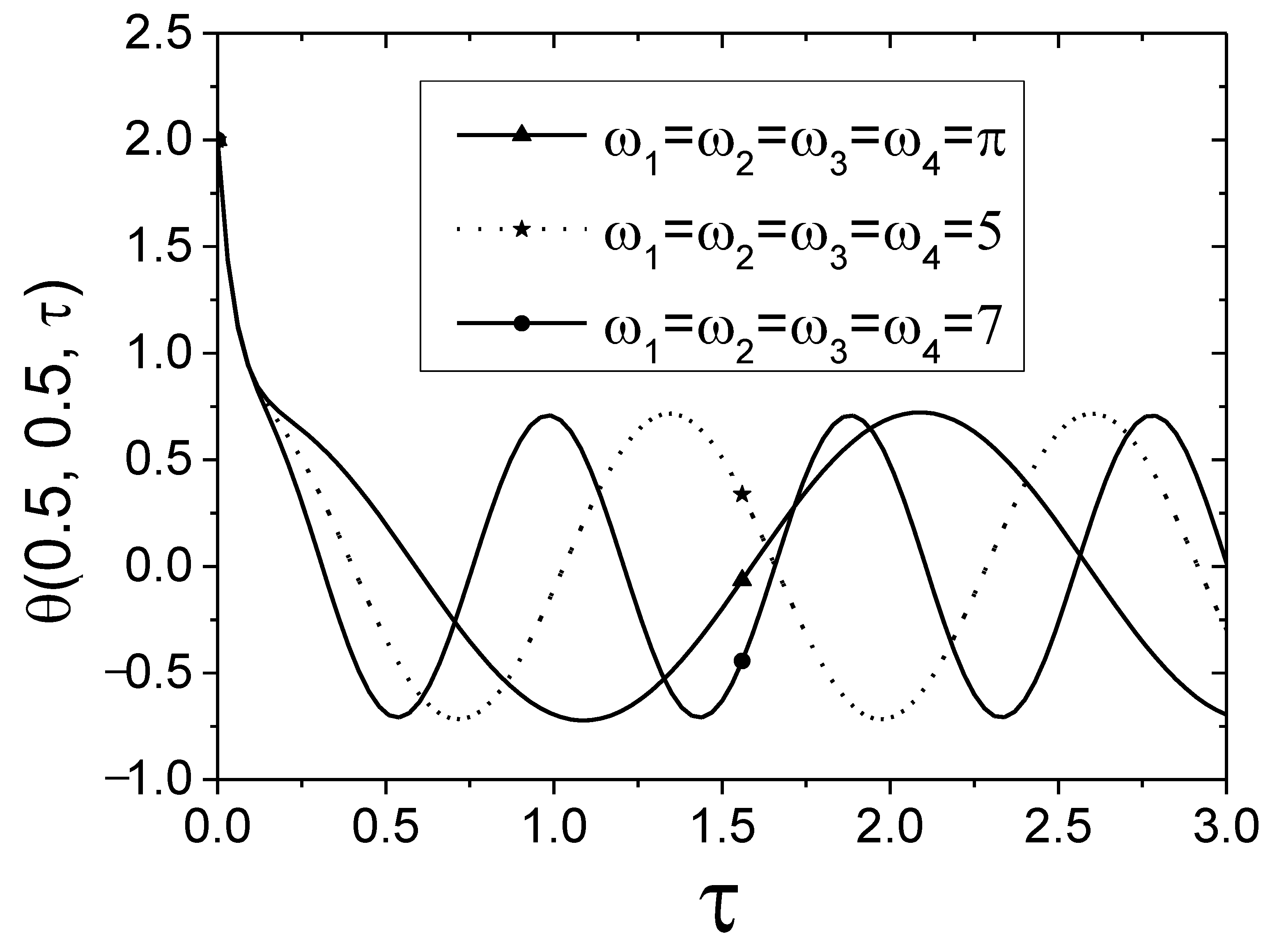
(3)
When considering the time-dependent boundary of harmonic function, the fluctuation of the temperature variation increases as the frequency of the harmonic function increases. When considering the time-dependent boundary of exponential function, e d i τ , a smaller coefficient d i will result in a lower and faster drop in temperature.
The analytic solution for the 2D heat conduction problems with general Dirichlet boundary conditions is obtained using the proposed method. However, the values of the boundary conditions and initial condition at the four corners of the rectangular region should be zero, which limits the applicability of this study. Transforming the temperature function before using the method proposed in this paper may overcome this limitation. A method that can be applied to the case for non-zero values at the four corners will be proposed in the near future.

Author Contributions

Conceptualization, T.-W.T. and J.-R.C.; formal analysis, H.-P.H.; investigation, J.-R.C.; methodology, H.-P.H., T.-W.T. and J.-R.C.; software, H.-P.H.; supervision, T.-W.T.; validation, J.-R.C.; writing—original draft, T.-W.T.; writing—review and editing, J.-R.C. All authors have read and agreed to the published version of the manuscript.

Funding

This research received no external funding. And the APC was funded by H.-P.H. and J.-R.C.

Data Availability Statement

Not applicable.

Conflicts of Interest

The authors declare no conflict of interest.

Nomenclature

A , B two subsystems
c specific heat ( W s / kg °C)
d i ( i = 1 , 2 , 3 , 4 ) four arbitrary constants
f i ( y , t ) , i = 1 , 2 temperatures along the surface at the left end and the right end of the rectangular region
f i ( x , t ) , i = 3 , 4 temperatures along the surface at the bottom end and the top end of the rectangular region
F i ( Y , τ ) , i = 1 , 2 dimensionless quantity defined in Equation (8)
F i ( X , τ ) , i = 3 , 4 dimensionless quantity defined in Equation (8)
F ¯ i , m ( τ ) , i = 1 , 2 dimensionless quantity defined in Equation (31)
F ¯ i , m ( τ ) , i = 3 , 4 dimensionless quantity defined in Equation (A7)
g i , m ( X ) , i = 1 , 2 shifting function
g i , m ( Y ) , i = 3 , 4 shifting function
G ¯ m ( X , τ ) nonhomogeneous term in the differential equation of the transformed system defined in Equation (43)
k thermal conductivity ( W / m °C)
L r aspect ratio, L y / L x defined in Equation (8)
L x , L y thickness of the two-dimensional rectangular region at x- and y- directions (m)
T ( x , y , t ) temperature function (°C)
T m n a ( τ ) , T m n b ( τ ) dimensionless time variable of the transformed function defined in Equations (53) and (A22)
T r reference temperature (°C)
T 0 ( x , y ) initial temperature (°C)
t time variable (s)
x space variable in x-direction of a rectangular region (m)
X dimensionless space variable in x-direction of a rectangular region
y space variable in y-direction of a rectangular region (m)
Y dimensionless space variable in y-direction of a rectangular region
α thermal diffusivity ( m 2 / s )
ϕ auxiliary integration variable
γ m n a ( τ ) , γ m n b ( τ ) dimensionless quantity defined in Equations (55) and (A24)
η i ( i = 1 , 2 , 3 , 4 ) time-dependent boundary condition
λ m n a , λ m n b n-th eigenvalues depend on ω n defined in Equations (54) and (A23)
θ dimensionless temperature
θ 0 dimensionless initial temperature
θ a , θ b dimensionless temperatures for subsystems A and B
θ m ( X , τ ) generalized Fourier coefficient defined in Equation (29)
θ ¯ m ( X , τ ) transformed function defined in Equation (36)
θ ¯ m n ( X , τ ) n-th eigenfunction of the transformed function defined in Equation (47)
ρ density ( kg / m 3 )
τ dimensionless time
ω n n-th eigenvalue for Sturm–Liouville problem defined in Equation (48).
Subscripts
0 , 1 , 2 , 3 , 4 , a , b , i , m , n , r described in the article

Appendix A. Analytic Solution of the Subsystem B

For the subsystem B , the boundary value problem is as follows:
[ L r 2 2 θ b ( X , Y , τ ) X 2 + 2 θ b ( X , Y , τ ) Y 2 ] = θ b ( X , Y , τ ) τ       in   0 < X < 1 , 0 < Y < 1 ,       τ > 0 ,
θ b ( 0 , Y , τ ) = 0 ,             θ b ( 1 , Y , τ ) = 0 ,
θ b ( X , 0 , τ ) = F 3 ( X , τ ) ,             θ b ( X , 1 , τ ) = F 4 ( X , τ ) ,
θ b ( X , Y , 0 ) = θ 0 ( X , Y ) θ a 0 ( X , Y ) = θ b 0 ( X , Y ) .
Because the boundary conditions of the rectangular region at two opposite edges X = 0 and X = 1 are homogeneous, the temperature θ b ( X , Y , τ ) and the dimensionless quantities F 3 ( X , τ ) , F 4 ( X , τ ) defined in Equation (A3), can be expressed as
θ b ( X , Y , τ ) = m = 1 [ θ m ( Y , τ ) sin ( m π X ) ] ,
F i ( X , τ ) = m = 1 [ F ¯ i , m ( τ ) sin ( m π X ) ] ,             ( i = 3 , 4 )
where m denotes a positive integer and F ¯ i , m ( τ ) ( i = 3 , 4 ) is given as
F ¯ i , m ( τ ) = 2 0 1 F i ( X , τ ) sin ( m π X ) d X , ( i = 3 , 4 ) .
Substituting Equations (A5) and (A6) back into Equations (A1)–(A4), one obtains
θ m ( Y , τ ) τ 2 θ m ( Y , τ ) Y 2 + m 2 π 2 L r 2 θ m ( Y , τ ) = 0 ,
θ m ( 0 , τ ) = F ¯ 3 , m ( τ ) ,             θ m ( 1 , τ ) = F ¯ 4 , m ( τ ) ,
θ m ( Y , 0 ) = 2 0 1 θ b 0 ( X , Y ) sin ( m π X ) d X .
To find the solution for the second-order differential Equation (A8) with nonhomogeneous boundary conditions (A9), one uses the shifting function method by taking
θ m ( Y , τ ) = θ ¯ m ( Y , τ ) + i = 3 4 g i , m ( Y ) F ¯ i , m ( τ )
where θ ¯ m ( Y , τ ) is the transformed function while g i , m ( Y ) ( i = 3 , 4 ) indicates the shifting function to be specified.
Substituting Equation (A11) back into Equations (A8)–(A10), one obtains
θ ¯ ˙ m ( Y , τ ) + i = 3 4 g i , m ( Y ) F ¯ ˙ i , m ( τ ) [ θ ¯ m ( Y , τ ) + i = 3 4 g i , m ( Y ) F ¯ i , m ( τ ) ] + m 2 π 2 L r 2 [ θ ¯ m ( Y , τ ) + i = 3 4 g i , m ( Y ) F ¯ i , m ( τ ) ] = 0 .
The associated boundary conditions become
θ ¯ m ( 0 , τ ) + g 3 , m ( 0 ) F ¯ 3 , m ( τ ) + g 4 , m ( 0 ) F ¯ 4 , m ( τ ) = F ¯ 3 , m ( τ ) ,
θ ¯ m ( 1 , τ ) + g 3 , m ( 1 ) F ¯ 3 , m ( τ ) + g 4 , m ( 1 ) F ¯ 4 , m ( τ ) = F ¯ 4 , m ( τ )
As in the derivation process, the two shifting functions are determined as
g 3 , m ( Y ) = 1 Y ,             g 4 , m ( Y ) = Y .
After substituting Equation (A15) into Equations (A12)–(A14), one has the differential equation for θ ¯ m ( Y , τ ) as
θ ¯ ˙ m ( Y , τ ) θ ¯ m ( Y , τ ) + m 2 π 2 L r 2 θ ¯ m ( Y , τ ) = G ¯ m ( Y , τ ) ,
and the associated homogeneous boundary conditions as
θ ¯ m ( 0 , τ ) = 0 ,             θ ¯ m ( 1 , τ ) = 0 .
G ¯ m ( Y , τ ) is defined as
G ¯ m ( Y , τ ) = i = 3 4 [ m 2 π 2 L r 2 g i , m ( Y ) F ¯ i , m ( τ ) + g i , m ( Y ) F ¯ ˙ i , m ( τ ) ] .
Moreover, the initial condition is transformed to be
θ ¯ m ( Y , 0 ) = 2 0 1 θ b 0 ( X , Y ) sin ( m π X ) d X i = 3 4 [ g i , m ( Y ) F ¯ i , m ( 0 ) ] .
The solution θ ¯ m ( Y , τ ) specified by Equations (A16)–(A19) can be expressed in the form of eigenfunctions as
θ ¯ m ( Y , τ ) = n = 1 θ ¯ m n ( Y ) T m n b ( τ )
where θ ¯ m n ( Y ) is
θ ¯ m n ( Y ) = sin n π Y .
Substituting Equation (A20) into Equation (A16), multiplying it by θ ¯ m n ( Y ) , and integrating from 0 to 1, one will obtain
T ˙ m n b ( τ ) + λ m n b 2 T m n b ( τ ) = γ m n b ( τ )
where λ m n b and γ m n b ( τ ) are
λ m n b = m 2 L r 2 + n 2 π ,
γ m n b ( τ ) = 2 0 1 θ ¯ m n ( Y ) G ¯ m ( Y , τ ) d Y = 2 n π { [ F ¯ ˙ 3 , m ( τ ) ( 1 ) n F ¯ ˙ 4 , m ( τ ) ] + m 2 π 2 L r 2 [ F ¯ 3 , m ( τ ) ( 1 ) n F ¯ 4 , m ( τ ) ] } .
Note that T m n b ( 0 ) can be determined from the initial condition of the transformed function defined in Equation (A19) as
T m n b ( 0 ) = 4 0 1 sin ( n π Y ) 0 1 θ b 0 ( X , Y ) sin ( n π X ) d X d Y 2 n π [ F ¯ 3 , m ( 0 ) ( 1 ) n F ¯ 4 , m ( 0 ) ] .
The general solution of Equation (A22) with the initial condition above is
T m n b ( τ ) = e λ m n b 2 τ T m n b ( 0 ) + 0 τ e λ m n b 2 ( τ ϕ ) γ m n b ( ϕ ) d ϕ .

References

  1. Perakis, N.; Haidna, O.J.; Ihme, M. Heat transfer augmentation by recombination reactions in turbulent reacting boundary layers at elevated pressures. Int. J. Heat Mass Transf. 2021, 178, 121628. [Google Scholar] [CrossRef]
  2. Hassan, M.A.S.M.; Razlan, Z.M.; Bakar, S.A.; Rahman, A.A.; Rojan, M.A.; Wan, W.K.; Ibrahim, Z.; Ishak, A.A.; Ridzuan, M.J.M. Derivation and validation of heat transfer model for Spark-Ignition engine cylinder head. Appl. Therm. Eng. 2023, 225, 120240. [Google Scholar] [CrossRef]
  3. Ivanov, V.; Salomatov, V. On the calculation of the temperature field in solids with variable heat-transfer coefficients. J. Eng. Phys. Thermophys. 1965, 72, 63–64. [Google Scholar] [CrossRef]
  4. Ivanov, V.; Salomatov, V. Unsteady temperature field in solid bodies with variable heat transfer coefficient. J. Eng. Phys. Thermophys. 1966, 11, 151–152. [Google Scholar] [CrossRef]
  5. Postol’Nik, Y.S. One-dimensional convective heating with a time-dependent heat-transfer coefficient. J. Eng. Phys. Thermophys. 1970, 18, 233–238. [Google Scholar] [CrossRef]
  6. Kozlov, V. Solution of heat-conduction problem with variable heat-exchange coefficient. J. Eng. Phys. Thermophys. 1970, 18, 100–104. [Google Scholar] [CrossRef]
  7. Holy, Z. Temperature and stresses in reactor fuel elements due to time-and space-dependent heat-transfer coefficients. Nucl. Eng. Des. 1972, 18, 145–197. [Google Scholar] [CrossRef]
  8. Özişik, M.N.; Murray, R. On the solution of linear diffusion problems with variable boundary condition parameters. J. Heat Transf. 1974, 96, 48–51. [Google Scholar] [CrossRef]
  9. Moitsheki, R.J. Transient heat diffusion with temperature-dependent conductivity and time-dependent heat transfer coefficient. Math. Probl. Eng. 2008, 9, 41–58. [Google Scholar] [CrossRef]
  10. Chen, H.T.; Sun, S.L.; Huang, H.C.; Lee, S.Y. Analytic closed solution for the heat conduction with time dependent heat convection coefficient at one boundary. Comput. Model. Eng. Sci. 2010, 59, 107–126. [Google Scholar]
  11. Lee, S.Y.; Huang, C.C. Analytic solutions for heat conduction in functionally graded circular hollow cylinders with time-dependent boundary conditions. Math. Probl. Eng. 2013, 5, 816385. [Google Scholar] [CrossRef]
  12. Lee, S.Y.; Tu, T.W. Unsteady temperature field in slabs with different kinds of time-dependent boundary conditions. Acta Mech. 2015, 226, 3597–3609. [Google Scholar] [CrossRef]
  13. Lee, S.Y.; Lin, S.M. Dynamic analysis of nonuniform beams with time-dependent elastic boundary conditions. J. Appl. Mech. 1996, 63, 474–478. [Google Scholar] [CrossRef]
  14. Lee, S.Y.; Huang, T.W. A method for inverse analysis of laser surface heating with experimental data. Int. J. Heat Mass Transf. 2014, 72, 299–307. [Google Scholar] [CrossRef]
  15. Lee, S.Y.; Huang, T.W. Inverse analysis of spray cooling on a hot surface with experimental data. Int. J. Therm. Sci. 2016, 100, 145–154. [Google Scholar] [CrossRef]
  16. Lee, S.Y.; Yan, Q.Z. Inverse analysis of heat conduction problems with relatively long heat treatment. Int. J. Heat Mass Transf. 2017, 105, 401–410. [Google Scholar] [CrossRef]
  17. Carslaw, H.; Jaeger, J. Heat in Solids, 2nd ed.; Clarendon Press: Oxford, UK, 1959. [Google Scholar]
  18. Özışık, M.N. Heat Conduction; John Wiley & Sons: New York, USA, 1993. [Google Scholar]
  19. Cole, K.D.; Beck, J.V.; Haji-Sheikh, A.; Litkouhi, B. Heat Conduction Using Green’s Functions; Taylor & Francis: Boca Raton, FL, USA, 2010. [Google Scholar]
  20. Zhu, S.P. Solving transient diffusion problems: Time-dependent fundamental solution approaches versus LTDRM approaches. Eng. Anal. Bound. Elem. 1998, 21, 87–90. [Google Scholar] [CrossRef]
  21. Zhu, S.P.; Liu, H.W.; Lu, X.P. A combination of LTDRM and ATPS in solving diffusion problems. Eng. Anal. Bound. Elem. 1998, 21, 285–289. [Google Scholar] [CrossRef]
  22. Sutradhar, A.; Paulino, G.H.; Gray, L. Transient heat conduction in homogeneous and non-homogeneous materials by the Laplace transform Galerkin boundary element method. Eng. Anal. Bound. Elem. 2002, 26, 119–132. [Google Scholar] [CrossRef]
  23. Bulgakov, V.; Šarler, B.; Kuhn, G. Iterative solution of systems of equations in the dual reciprocity boundary element method for the diffusion equation. Int. J. Numer. Methods Eng. 1998, 43, 713–732. [Google Scholar] [CrossRef]
  24. Walker, S. Diffusion problems using transient discrete source superposition. Int. J. Numer. Methods Eng. 1992, 35, 165–178. [Google Scholar] [CrossRef]
  25. Chen, C.; Golberg, M.; Hon, Y. The method of fundamental solutions and quasi-Monte-Carlo method for diffusion equations. Int. J. Numer. Methods Eng. 1998, 43, 1421–1435. [Google Scholar] [CrossRef]
  26. Burgess, G.; Mahajerin, E. Transient heat flow analysis using the fundamental collocation method. Appl. Therm. Eng. 2003, 23, 893–904. [Google Scholar] [CrossRef]
  27. Young, D.; Tsai, C.; Murugesan, K.; Fan, C.; Chen, C. Time-dependent fundamental solutions for homogeneous diffusion problems. Eng. Anal. Bound. Elem. 2004, 28, 1463–1473. [Google Scholar] [CrossRef]
  28. Cole, K.D.; Yen, D.H. Green’s functions, temperature and heat flux in the rectangle. Int. J. Heat Mass Transf. 2001, 44, 3883–3894. [Google Scholar] [CrossRef]
  29. Beck, J.V.; Wright, N.T.; Haji-Sheikh, A. Transient power variation in surface conditions in heat conduction for plates. Int. J. Heat Mass Transf. 2008, 51, 2553–2565. [Google Scholar] [CrossRef]
  30. Lei, J.; Wang, Q.; Liu, X.; Gu, Y.; Fan, C.-M. A novel space-time generalized FDM for transient heat conduction problems. Eng. Anal. Bound. Elem. 2020, 119, 1–12. [Google Scholar] [CrossRef]
  31. Alam, M.N.; Tunç, C. New solitary wave structures to the (2 + 1)-dimensional KD and KP equations with spatio-temporal dispersion. J. King Saud Univ. Sci. 2020, 32, 3400–3409. [Google Scholar] [CrossRef]
  32. Islam, S.; Alam, M.N.; Fayz-Al-Asad, M.; Tunç, C. An analytical technique for solving new computational solutions of the modified Zakharov-Kuznetsov equation arising in electrical engineering. J. Appl. Comput. Mech. 2021, 7, 715–726. [Google Scholar]
  33. Krishnan, G.; Parhizi, M.; Jain, A. Eigenfunction-based solution for solid-liquid phase change heat transfer problems with time-dependent boundary conditions. Int. J. Heat Mass Transf. 2022, 189, 122693. [Google Scholar] [CrossRef]
  34. Belekar, V.V.; Murphy, E.J.; Subramaniam, S. Analytical solution to heat transfer in stationary wet granular mixtures with time-varying boundary conditions. Int. Commun. Heat Mass Transf. 2023, 140, 106500. [Google Scholar] [CrossRef]
Figure 1. The 2D heat conduction in a rectangular cross-section of an infinite bar with general Dirichlet boundary conditions. (a) An infinite bar with a rectangular cross-section. (b) The 2D heat transfer system in a rectangular region (cross-section).
Axioms 12 00416 g001
Figure 2. The two subsystems of the two-dimensional heat conduction system with general Dirichlet boundary conditions. (a) For subsystem A. (b) For subsystem B.
Axioms 12 00416 g002
Figure 3. Temperature variation in the middle of the rectangular region with various parameters of harmonic-type time-dependent boundary conditions (Case 2 of Example 1).
Axioms 12 00416 g003
Figure 4. Temperature variation in the middle of the rectangular region with various parameters of exponential-type time-dependent boundary conditions (Example 2).
Axioms 12 00416 g004
Table 1. The temperature of the rectangular region at X = Y = 0.5 and at various times [ η i ( τ ) = e τ , ( i = 1 , 2 , 3 , 4 ) ].
τ θ ( X = 0.5 , Y = 0.5 , τ )
Number   of   Expansion   Terms   ( m = n )
1351020
00.5160.4970.5010.5000.500
0.10.2290.2460.2430.2430.243
0.20.1740.1890.1870.1870.187
0.40.1380.1500.1480.1480.148
0.60.1130.1230.1210.1210.121
0.80.09210.1000.09890.09940.0994
1.00.07540.08230.08100.08140.0814
1.20.06180.06740.06630.06660.0666
Table 2. The temperature of the rectangular region at X = Y = 0.5 and at various times [ η i ( τ ) = e τ , ( i = 1 , 2 ) ; η i ( τ ) = e 2 τ , ( i = 3 , 4 ) ].
τ θ ( X = 0.5 , Y = 0.5 , τ )
Number   of   Expansion   Terms   ( m = n )
1351020
00.5160.4970.5010.5000.500
0.10.2490.2630.2610.2610.261
0.20.2030.2150.2130.2130.213
0.40.1760.1840.1830.1830.183
0.60.1540.1590.1590.1590.159
0.80.1330.1360.1360.1360.136
1.00.1130.1150.1150.1150.115
1.20.09540.09690.09670.09680.0968
Table 3. The temperature of the rectangular region at X = Y = 0.5 and at various times [ η i ( τ ) = e i τ , ( i = 1 , 2 , 3 , 4 ) ].
τ θ ( X = 0.5 , Y = 0.5 , τ )
Number   of   Expansion   Terms   ( m = n )
1351020
00.5160.4970.5010.5000.500
0.10.2850.2950.2930.2930.293
0.20.2510.2570.2560.2560.256
0.40.2290.2300.2300.2300.230
0.60.2020.2010.2020.2020.202
0.80.1740.1720.1720.1720.172
1.00.1470.1450.1460.1460.146
1.20.1230.1210.1220.1220.122
Disclaimer/Publisher’s Note: The statements, opinions and data contained in all publications are solely those of the individual author(s) and contributor(s) and not of MDPI and/or the editor(s). MDPI and/or the editor(s) disclaim responsibility for any injury to people or property resulting from any ideas, methods, instructions or products referred to in the content.

