
Aperiodic Sampled-Data Control for Anti-Synchronization of Chaotic Nonlinear Systems Subject to Input Saturation


1
College of Mathematic Science, Shandong University of Science and Technology, Qingdao 266590, China
2
College of Electrical Engineering and Automation, Shandong University of Science and Technology, Qingdao 266590, China
*
Author to whom correspondence should be addressed.
Axioms 2023, 12(4), 403; https://doi.org/10.3390/axioms12040403
Submission received: 29 March 2023
/
Revised: 16 April 2023
/
Accepted: 19 April 2023
/
Published: 21 April 2023
(This article belongs to the Topic Advances in Nonlinear Dynamics: Methods and Applications)
Abstract
:This paper studies the aperiodic sampled-data (SD) control anti-synchronization issue of chaotic nonlinear systems under the effects of input saturation. At first, to describe the simultaneous existence of the aperiodic SD pattern and the input saturation, a nonlinear closed-loop system model is established. Then, to make the anti-synchronization analysis, a relaxed sampling-interval-dependent Lyapunov functional (RSIDLF) is constructed for the resulting closed-loop system. Thereinto, the positive definiteness requirement of the RSIDLF is abandoned. Due to the indefiniteness of RSIDLF, the discrete-time Lyapunov method (DTLM) then is used to guarantee the local stability of the trivial solutions of the modeled nonlinear system. Furthermore, two convex optimization schemes are proposed to expand the allowable initial area (AIA) and maximize the upper bound of the sampling period (UBSP). Finally, two examples of nonlinear systems are provided to illustrate the superiority of the RSIDLF method over the previous methods in expanding the AIA and enlarging the UBSP.
1. Introduction
The concept of chaotic synchronization of master–slave systems was proposed in the last century. Up to now, the chaotic synchronization issue has been extensively studied and has been widely used in many fields [1,2], such as secure communication and biochemistry. There are a variety of types chaotic synchronization, including but not limited to complete synchronization [3,4,5,6,7], anti-synchronization [8,9,10,11,12], projective synchronization [13,14,15], and generalized synchronization [16,17,18]. As an interesting chaotic synchronization behavior, anti-synchronization refers to the state vectors of the master–slave systems having the same absolute value but with opposite sign. Recently, anti-synchronization has been widely studied. For example, Ref. [8] has investigated the anti-synchronization problem of hyperchaotic Chua systems, Ref. [9] has discussed the finite-time anti-synchronization issue for a class of coupled neural networks, Ref. [10] has addressed the anti-synchronization of switched inertial neural networks, etc. Moreover, nonlinear systems have been gaining more and more attention in recent decades [19,20,21]. To the best of our knowledge, the theory and applications of linear systems are far more mature and complete than those of nonlinear systems. However, linear systems absolutely do not exist in practical applications because all components of the practical system have nonlinear properties to varying degrees. Indeed, the research of nonlinear systems will be more complicated compared with simple linear systems. What is more, many practical examples, such as neural networks and Chua systems, can be classified as nonlinear systems. It is, therefore, necessary and challenging to study the anti-synchronization of nonlinear systems.
Looking through the excellent works in the control field, e.g., adaptive control and state feedback control, there are many classical and effective synchronization control methods. However, the common characteristic of these control methods is that they are all point-to-point control, which will inevitably give rise to the excessive occupation of communication channels. Followed by the booming of network technology, networked control methods have emerged due to their advantages in energy saving; these methods include SD control [22,23,24,25,26], intermittent control [27,28], quantized control [29,30], even-triggered control [31,32,33], and so on. Thereinto, the SD controllers deliver control signals at a range of discrete instants . As such, SD control has become an economic and welcome approach given the booming of networks and multimedia digital technologies. Note that under periodic SD control, signals are usually sampled in a fixed period. However, considering some adverse factors, that is, the unstable voltage source from the physical environment, the sampler used may vibrate slightly, and the actual sampling period will undulate within a limited period. Therefore, it is very necessary to study the stability analysis of closed-loop systems under aperiodic SD control. As an example, the exponential synchronization issue of neural networks has been discussed by using the aperiodic SD control in [22], and aperiodic SD synchronization has been discussed for delayed Lur’e systems in [24]. In addition, aperiodic SD synchronization has been studied for delayed stochastic Markovian jump neural networks in [25] and the quasi-synchronization of heterogeneous harmonic oscillators has been investigated under an aperiodic SD scheme in [26]. Nevertheless, the above works are obtained without considering the input saturation. In fact, actuators often experience a saturation phenomenon due to the physical constraints of the components [34]. This nonlinear characteristic might give rise to oscillation or even instabilities of the saturation control systems. Therefore, it is of great importance to analyze the design of saturated aperiodic SD controllers. Although it has an engineering background, so far, there is little research on the local anti-synchronization of nonlinear systems with input saturation by utilizing aperiodic SD control.
On the other hand, in the SD control closed-loop systems, the continuous and discrete signals exist simultaneously. From the viewpoint of control theory, it will bring substantial challenges in the analysis and synthesis of SD control systems. In recent years, a breed of sampling-interval-dependent Lyapunov functionals (SIDLFs) has been constructed for discussing the local stability of various systems under SD. In comparison with the traditional quadratic Lyapunov–Krasovskii functional, the SIDLF makes full use of the state’s information within the sampling intervals. Obviously, this will help to improve the stability results. For example, an SIDLF is constructed and the input delay approach has been utilized to investigate the SD control linear systems in [35]. In addition, a novel SIDLF has been constructed for the delayed neural networks to study the exponential synchronization problems in [22]. To further improve the results, an RSIDLF, where the positive definiteness is not required within the sampling intervals, has been established for linear SD control systems [36]. After that, an RSIDLF has been established to carry out the stability analysis of linear systems under aperiodic SD control [37]. Furthermore, the RSIDLF has been employed to deal with the aperiodic SD control exponential stabilization of delayed neural networks in [38]. Nonetheless, these works do not take the input saturation into account. Namely, the proposed analysis approaches cannot be applied in saturated control systems. Inspired by these existing works, two interesting problems naturally arise: whether can we construct a joint strategy where not only a novel RSIDLF for local stability of closed-loop nonlinear systems is designed but also the satisfactory anti-synchronization performance to satisfy the demand caused by the saturated aperiodic SD control can be guaranteed. How can we quantitatively analyze the superiority of the RSIDLF over the traditional SIDLF? Thus, how can we handle these problems well enough to motivate the present discussion of this paper.
According to the discussion above, this paper addresses the anti-synchronization issue of chaotic nonlinear systems via aperiodic SD control considering input saturation. The research works and contributions are mainly concluded as follows.
(1) Taking the characteristics of the aperiodic SD scheme into consideration, a novel SIDLF is newly designed to carry out some less conservative results for the local stability of nonlinear systems. It should be mentioned that the positive definite restrictions of the RSIDLF are discarded. As an alternative, the RSIDLF is only required to be positive definite at the discrete sampling instants.
(2) Under the RSIDLF, in combination with the DTLM, the squeeze theory, and some inequality estimation techniques, two improved criteria are derived for closed-loop nonlinear systems under saturated aperiodic SD control.
(3) Aiming at enlarging the AIA and maximizing the UBSP, two optimization algorithms are designed. With the help of the devised optimization algorithms, two comparative analyses between the RSIDLF and the existing results are provided.
The outline of this paper is as follows. Section 2 gives some preliminaries and presents an aperiodic SD scheme and system model. Section 3 presents the main results on stability and stabilization of nonlinear systems by using the SD strategy. Section 4 designs two optimization algorithms to expand the AIA and maximize the UBSP. Two numerical examples are presented to verify the obtained results. Finally, Section 6 concludes this paper.
Notations. stands for the set of symmetric matrices. represents the set of positive definite and symmetric matrices. denotes the ith row of matrix W. and stand for a block diagonal matrix and a column vector. stands for inverse (transpose) of matrix W. denotes the maximal eigenvalue of matrix W. , is the p-norm of a vector or a matrix.
2. Preliminaries and Problem Formulation
Consider chaotic nonlinear systems as follows:
where denotes the state vector, matrices , and , the activation function .
Take the system (1) as the master system; the corresponding slave system is represented as
where denotes the state vector of the slave system, and the other items and matrices are the same as those in the master system; is the saturated control input.
Following the definition of the anti-synchronization, let . Then, the error system can be described as
where , and
with the control gain matrix and the sequence of sampling instants () satisfying , , satisfying . is the saturated nonlinear function, which is defined as
where denotes the saturation degree. denotes the ith row of the control gain matrix C.
Define a dead-zone nonlinear function [39] as
Then, rewrite system (3) as follows:
Next, define a polyhedral set
Next, an assumption and a lemma are presented as follows:
Assumption A1.
The nonlinear function is assumed to be odd, monotonically nondecreasing, and satisfies
Lemma 1
3. Main Results
In this section, several anti-synchronization criteria are derived by using an RSIDLF, some inequality techniques, and discrete-time Lyapunov method.
Theorem 1.
For given scalars and C, , if there exist matrices , diagonal matrices , and matrices , , enabling LMIs (7)–(9) to be satisfied for ,
where and , , ; other matrix blocks not mentioned are zero matrices with suitable dimensions, and Then, for any initial values , the trajectories of nonlinear systems (4) under aperiodic SD control can converge to zero. That is, the anti-synchronization of master system and slave system can be achieved.
Proof.
Differentiate for ; it holds that
Based on the Jensen’s inequality and Lemma 1, we can obtain
where .
In view of the Newton–Leibniz formulae, for matrices , and , we obtain
Furthermore, for any matrices , we can derive
In addition, there is a diagonal matrix , such that
In view of (6), one has
Combining with (8) and (9) and the convex combination technique [35], it can be inferred that if , , hold, , can be obtained. Thus, we can derive
Due to the indefiniteness of , we cannot directly draw the stability conclusion of the system (4). From (14), we have ; thus, . It should be noted that at instants , degenerates into and therefore satisfies the requirement of positive definiteness and strict decreasing. Thus, from the DTLM, it yields
which means
Next, the result that the trivial solution of system (4) is locally stable, i.e., small perturbations around an equilibrium point do not cause the system to move away from that point in the long term, for , will be proved. From the p-norm estimation method and (4), it follows that
In addition, according to the Cauchy–Schwarz inequality [40], it holds that
Remark 1.
It should be mentioned that the feature of the constructed functionals in Theorem 1 is that the states of information from to and from to are fully utilized. As a result, it has the ability to relax the conservatism of the stability conditions. On the other hand, the main difference between the constructed functionals in Theorem 1 and the previous functionals used in SIDLF [22,35,42] is that the positive definiteness constraints of Lyapunov matrices in functionals and are dropped. The previous functionals [22,35,42] will undoubtedly increase the conservatism of the results. That is, it can be believed that the results obtained based on the RSIDLF in Theorem 1 are superior to the results in [22,35,42].
Notice that if we set and , the designed relaxed functional will become positive, which is used in [22,35,42]. Then, aiming at displaying the advantage of the obtained results in Theorem 1, the following Corollary 1 is presented.
Corollary 1.
Proof.
With the conditions , , and (16), it holds that . Correspondingly, combined with the condition (14) and according to the CTLM, we can directly obtain that the trajectories of (4) can converge to zero for any initial values belonging to the . Namely, the locally asymptotical anti-synchronization of systems (1) and (2) with input saturation can be realized under the aperiodic SD scheme. The proof is completed. □
Remark 2.
It is worth noting that the main challenge in this paper is how to analyze the local stability of the trivial solutions of the error system (4) in Theorem 1. It is worth noting that the positive definiteness of the constructed RSIDLF between two adjacent sampling instants, i.e., , is no longer necessary. In this situation, the traditional Lyapunov–Krasovskii stability analysis method [22,35], i.e., is greater than 0, is less than 0, utilized in [22,35], can no longer be used to deal with the stability problem in Theorem 1. On the other hand, under the RSIDLF, the existing direct integration method [37] for linear SD control systems is also not applicable to the nonlinear systems. To overcome these challenges, the proof of Theorem 1 is divided into two steps.
- Step 1:
- Guaranteeing the stability of discrete instants with the help of the DTLM;
- Step 2:
- Estimating the trivial solutions inside the sampling interval by using the squeeze theory.
On this basis, combining the generalized sector condition with a series of inequality estimation approaches, a new local asymptotical anti-synchronization criterion is derived for closed-loop nonlinear system (4) under saturated aperiodic SD control.
In the following, in order to solve the control gain, the following criteria can be obtained.
Theorem 2.
For given scalars , if there exist , , , diagonal matrices , and matrices , , LMIs (17)–(19) are satisfied for ,
where and , , ; other matrix blocks not mentioned are zero matrices with suitable dimensions and Then, for any initial values with , the trajectories of nonlinear systems (4) under aperiodic SD control can converge to the zero. In addition, the gain matrix is given by .
Proof.
Define three partitioned diagonal matrices
and denote , , , , , , , , , , , , , .
Corollary 2.
Proof.
Remark 3.
From Theorems 1 and 2, it can be concluded that the estimated AIA is contained in the exact AIA. If , the inequality (7) implies that . Then, under the conditions of Theorems 1–2, it an be derived that . Hence, also belongs to . Repeating the above derivation, we can obtain the result that and hold for all . In consequence, it can be easily concluded that is indeed a positive invariant set as for the sampling states .
4. Optimization Algorithms
Due to the input saturation phenomenon and limited bandwidth, the larger AIA and the larger UBSP are more favorable. To handle these issues, the following two optimization algorithms in view of Theorem 2 and Corollary 2 are presented.
4.1. Optimization of the AIA
Given scalars , the aim is to obtain the largest AIA. Inspired by [39], the maximization of the minimal axis of the set is equal to the minimization of the value . To address this issue, the following optimization algorithm is designed:
then, it yields , and thus .
4.2. Optimization of the UBSP
Given AIA , the scalar , the aim is to maximize the UBSP . To solve this issue, the following optimization algorithm is designed:
Similar to the optimization algorithm in Section 4.1, the last LMI can guarantee .
5. Numerical Simulation
Example 1.
Set , (), , . Then, with help of the optimization scheme in Section 4 and the LMI toolbox in MATLAB, we obtain the results based on Corollary 2 (method in [22,35]) as , and the AIA
and the results based on the RSIDLF [22,28,35,42] as , , and the AIA
More clearly, the corresponding results are shown in Table 1 and Figure 2. One can see that the RSIDLF in Theorem 2 is helpful to expand the AIA indeed in comparison with Corollary 2 (method in [22,35]).
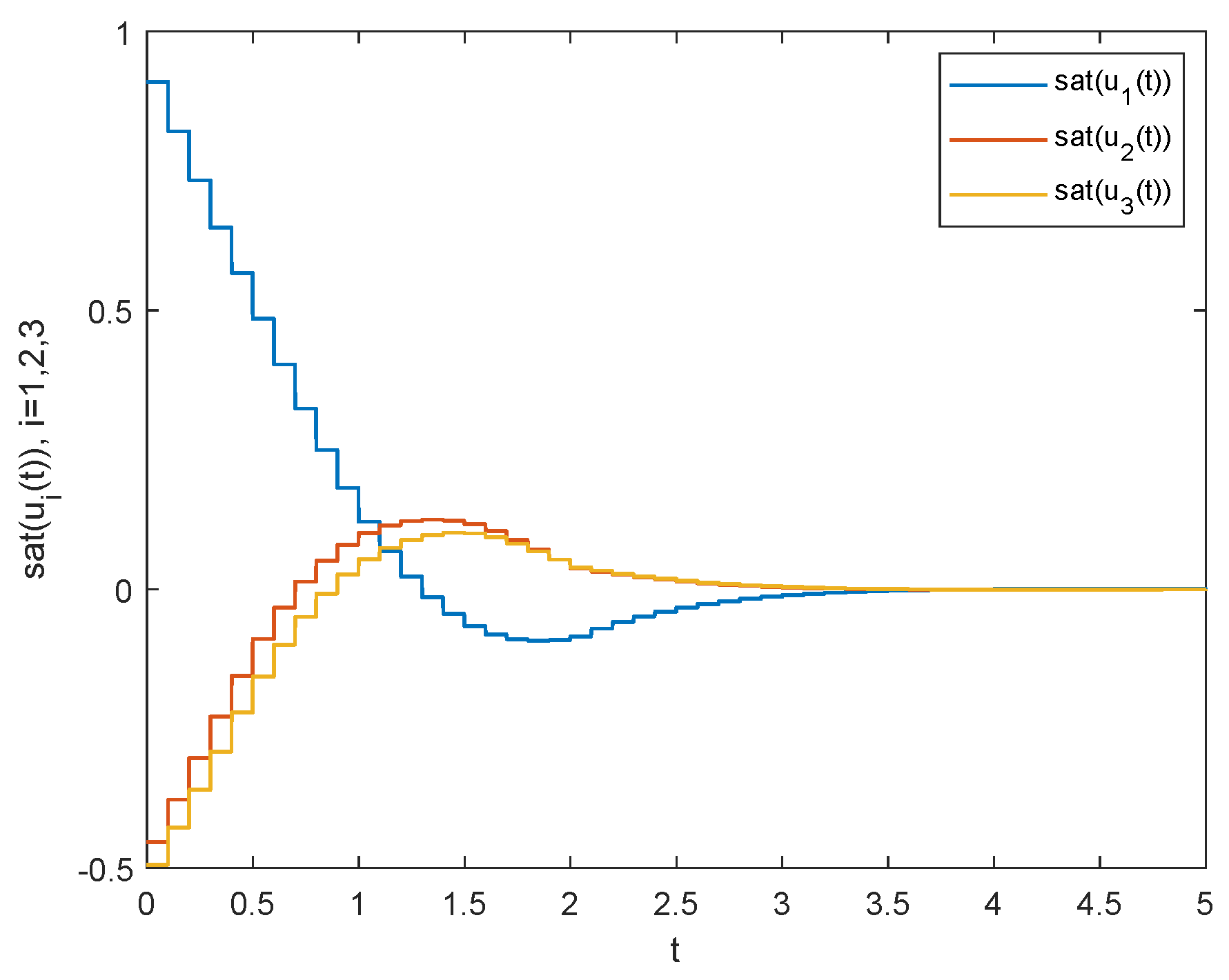
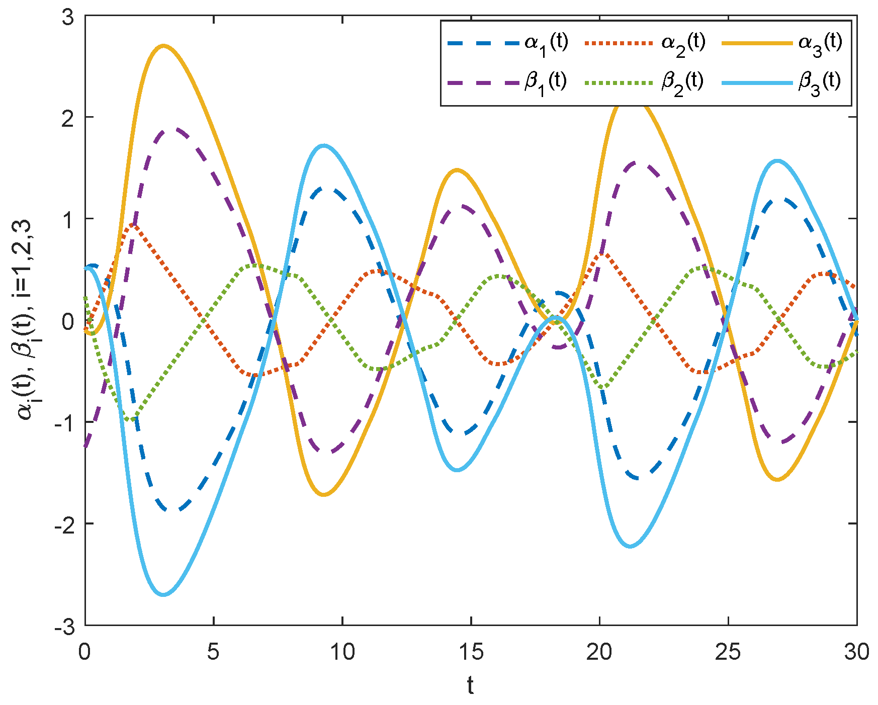
Take the initial value of the slave system as so that the initial value of the error system is belonging to the AIA . Then, the trajectories of the saturated aperiodic SD controller , the master system and the slave system , and the error system under the controller are shown in Figure 3, Figure 4 and Figure 5, respectively.
It can be seen that the error system and saturated aperiodic SD controller are each asymptotically stable. Furthermore, the master system and slave system are completely opposite as .
Example 2.
Based on optimization Section 4.2, select , (), , and ; then, in view of Theorem 2, one can obtain ,
and the AIA
It can be seen from the above results that, compared with Corollary 2, the RSIDLF in Theorem 2 is indeed conducive to improving the UBSP.
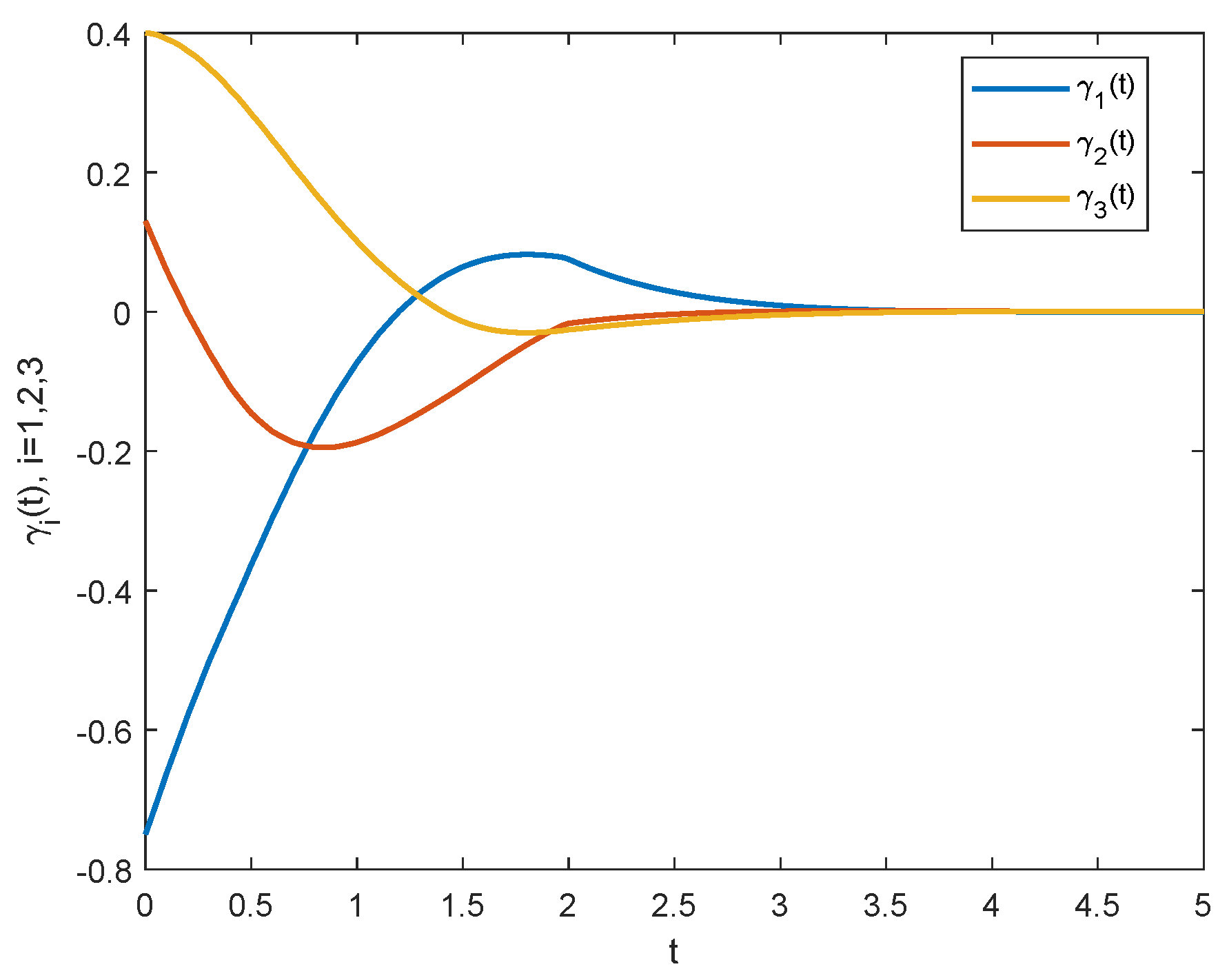
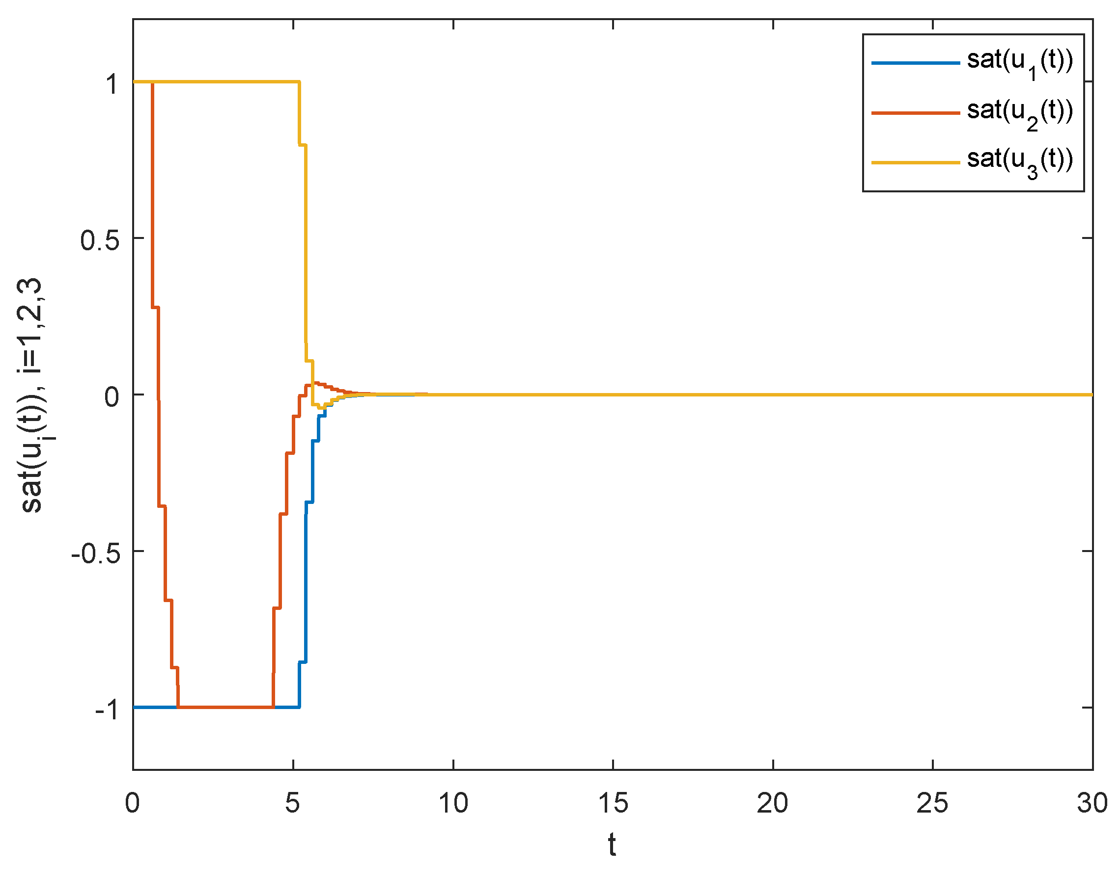
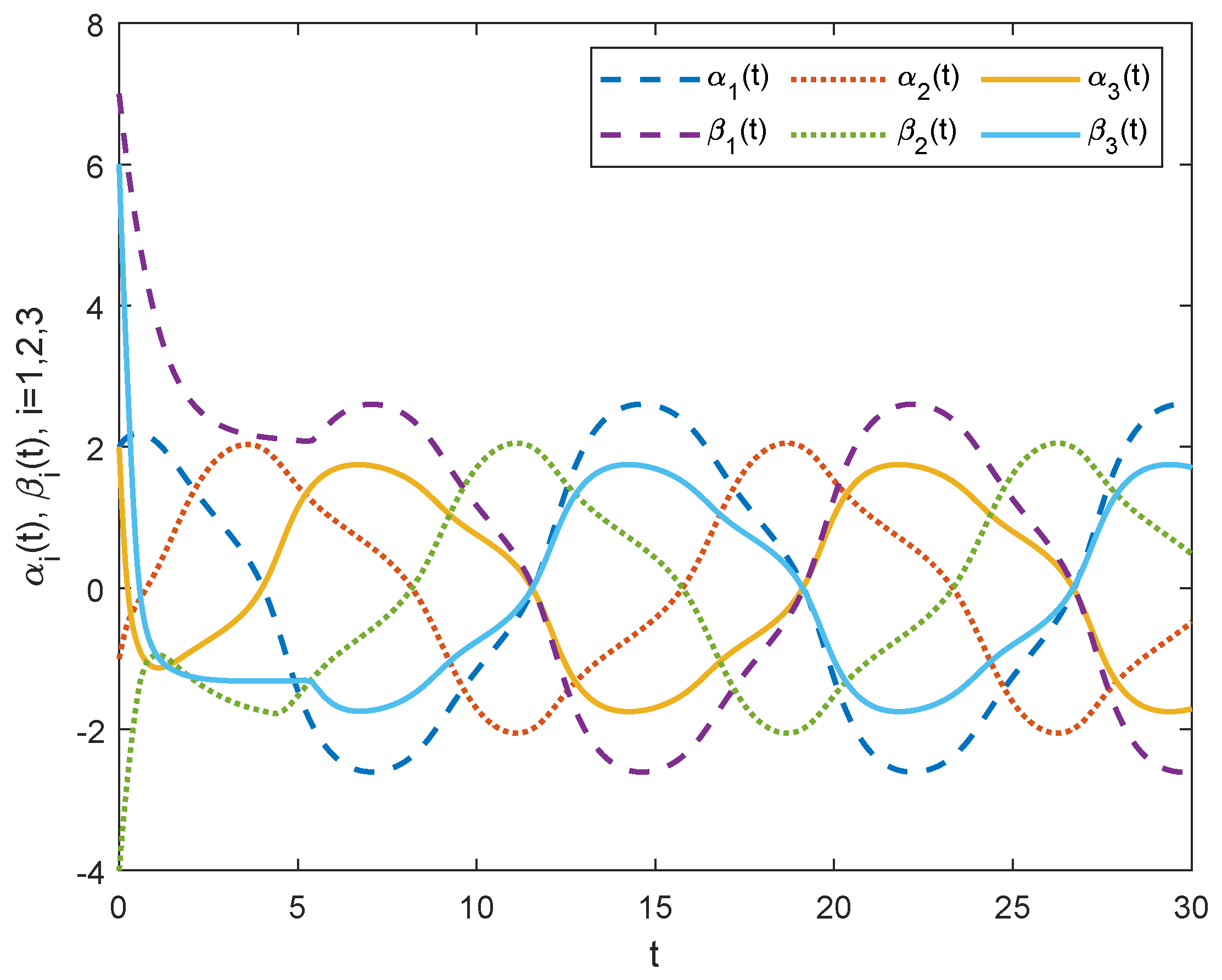
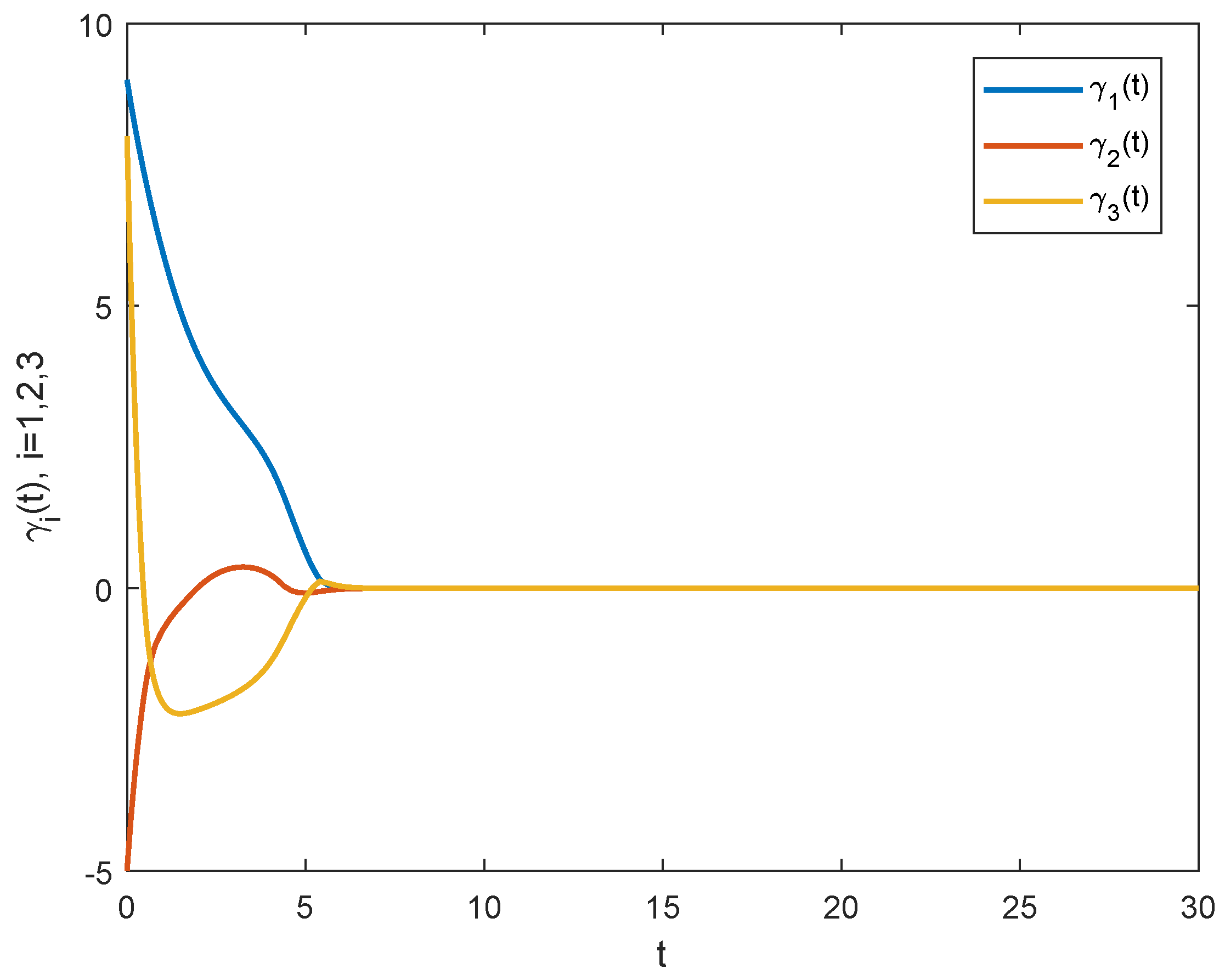
Take the initial value of the slave system as so that the initial value of the error system is belonging to the AIA . Then, the the saturated aperiodic SD controller , the master system and the slave system , and the error system under the saturated aperiodic SD controller are shown in Figure 6, Figure 7 and Figure 8, respectively.
It can be concluded that the designed saturated aperiodic SD controller has the ability to stabilize the error system as . That is, the anti-synchronization of master system and slave system can be achieved. It illustrates that although Theorem 2 relaxes the sufficient conditions to guarantee the anti-synchronization, the anti-synchronization between the master system and slave system can also be successfully achieved.
6. Conclusions
This article has been concerned with the anti-synchronization problem of chaotic nonlinear systems under aperiodic SD control subject to input saturation. In view of the characteristics of the aperiodic SD control, an RSIDLF which makes full use of the state information in sampling intervals has been newly designed. Then, the CTLM are utilized to derive the sufficient conditions to guarantee the local anti-synchronization of the master–slave systems. To expand the AIA and maximize the UBSP, two convex optimization schemes have been put forward. Two numerical examples of nonlinear systems have been presented to illustrate the advantages of the derived results compared with the previous methods. Our future work will pay attention to designing the lower conservative functional to study the anti-synchronization problem of nonlinear systems under event-triggered control and how to generalize our research to higher-order systems.
Author Contributions
Conceptualization and methodology, M.L.; writing—original draft preparation, Y.F.; funding acquisition, Y.F. All authors have read and agreed to the published manuscript.
Funding
This work was supported by the National Natural Science Foundation of China under Grants 62003794.
Institutional Review Board Statement
Not applicable.
Informed Consent Statement
Not applicable.
Data Availability Statement
Data sharing not applicable to this article as no datasets were generated or analyzed.
Acknowledgments
We would like to express our great appreciation to the editors and reviewers.
Conflicts of Interest
The authors declare no conflict of interest.
References
- Sun, J.; Zang, M.; Liu, P.; Wang, Y. A secure communication scheme of three-variable chaotic coupling synchronization based on DNA chemical reaction networks. IEEE Trans. Signal Process. 2022, 70, 2362–2373. [Google Scholar] [CrossRef]
- Kano, T.; Umeno, K. Chaotic synchronization of mutually coupled systems-arbitrary proportional linear relations. Chaos 2022, 32, 113137. [Google Scholar] [CrossRef]
- Jiang, H.; Zhuang, L.; Chen, C.; Wang, Z. Hidden dynamics and hybrid synchronization of fractional-order memristive systems. Axioms 2022, 11, 645. [Google Scholar] [CrossRef]
- Xin, L.; Shi, X.; Xu, M. Dynamical analysis and generalized synchronization of a novel fractional-order hyperchaotic system with hidden attractor. Axioms 2023, 12, 6. [Google Scholar] [CrossRef]
- Yan, S.; Gu, Z.; Park, J.H.; Xie, X. Synchronization of delayed fuzzy neural networks with probabilistic communication delay and its application to image encryption. IEEE Trans. Fuzzy Syst. 2023, 31, 930–940. [Google Scholar] [CrossRef]
- Dong, S.; Liu, X.; Zhong, S.; Shi, K.; Zhu, H. Practical synchronization of neural networks with delayed impulses and external disturbance via hybrid control. Neural Netw. 2023, 157, 54–64. [Google Scholar] [CrossRef] [PubMed]
- Si, X.; Wang, Z.; Fan, Y. Quantized control for finite-time synchronization of delayed fractional-order memristive neural networks: The Gronwall inequality approach. Expert Syst. Appl. 2023, 215, 119310. [Google Scholar] [CrossRef]
- Li, H.L.; Jiang, Y.L.; Wang, Z.L. Anti-synchronization and intermittent anti-synchronization of two identical hyperchaotic Chua systems via impulsive control. Nonlinear Dyn. 2015, 79, 919–925. [Google Scholar] [CrossRef]
- Hou, J.; Huang, Y.; Yang, E. Finite-time anti-synchronization of multi-weighted coupled neural networks with and without coupling delays. Neural Process. Lett. 2019, 50, 2871–2898. [Google Scholar] [CrossRef]
- Shi, J.; Zeng, Z. Anti-synchronization of delayed state-based switched inertial neural networks. IEEE Trans. Cybern. 2021, 51, 2540–2549. [Google Scholar] [CrossRef]
- Sakthivel, R.; Anbuvithya, R.; Mathiyalagan, K.; Ma, Y.K.; Prakash, P. Reliable anti-synchronization conditions for BAM memristive neural networks with different memductance functions. Appl. Math. Comput. 2016, 275, 213–228. [Google Scholar] [CrossRef]
- Yuan, M.; Wang, W.; Luo, X.; Liu, L.; Zhao, W. Finite-time anti-synchronization of memristive stochastic BAM neural networks with probabilistic time-varying delays. Chaos Solitons Fractals 2018, 113, 244–260. [Google Scholar] [CrossRef]
- Min, F.; Luo, A.C. Complex dynamics of projective synchronization of Chua circuits with different scrolls. Int. J. Bifurc. Chaos 2015, 25, 1530016. [Google Scholar] [CrossRef]
- Sun, J.; Shen, Y.; Zhang, X. Modified projective and modified function projective synchronization of a class of real nonlinear systems and a class of complex nonlinear systems. Nonlinear Dyn. 2014, 78, 1755–1764. [Google Scholar] [CrossRef]
- Zhang, W.; Sha, C.; Cao, J.; Wang, G.; Wang, Y. Adaptive quaternion projective synchronization of fractional order delayed neural networks in quaternion field. Appl. Math. Comput. 2021, 400, 126045. [Google Scholar] [CrossRef]
- Gasri, A.; Ouannas, A.; Ojo, K.S.; Pham, V.T. Coexistence of generalized synchronization and inverse generalized synchronization between chaotic and hyperchaotic systems. Nonlinear Anal. Model. Control. 2018, 23, 583–598. [Google Scholar] [CrossRef]
- Wang, D.; Huang, L.; Tang, L.; Zhuang, J. Generalized pinning synchronization of delayed Cohen-Grossberg neural networks with discontinuous activations. Neural Netw. 2018, 104, 80–92. [Google Scholar] [CrossRef]
- Huang, Y.; Chen, W.; Ren, S.; Zheng, Z. Analysis and pinning control for generalized synchronization of delayed coupled neural networks with different dimensional nodes. J. Frankl. Inst. 2018, 355, 5968–5997. [Google Scholar] [CrossRef]
- Shi, K.; Wang, B.; Yang, L.; Jian, S.; Bi, J. Takagi-Sugeno fuzzy generalized predictive control for a class of nonlinear systems. Nonlinear Dyn. 2017, 89, 169–177. [Google Scholar] [CrossRef]
- Califano, C.; Moog, C.H. Accessibility of nonlinear time-delay systems. IEEE Trans. Autom. Control. 2017, 62, 1254–1268. [Google Scholar] [CrossRef]
- Araújo, R.F.; Torres, L.A.; Palhares, R.M. Reinaldo Martine, Distributed control of networked nonlinear systems via interconnected Takagi-Sugeno fuzzy systems with nonlinear consequent. IEEE Trans. Syst. Man, Cybern. Syst. 2021, 51, 4858–4867. [Google Scholar] [CrossRef]
- Wu, Z.G.; Shi, P.; Su, H.; Chu, J. Exponential synchronization of neural networks with discrete and distributed delays under time-varying sampling. IEEE Trans. Neural Netw. Learn. Syst. 2012, 23, 1368–1376. [Google Scholar]
- Yan, S.; Gu, Z.; Park, J.H.; Xie, X. Sampled memory-event-triggered fuzzy load frequency control for wind power systems subject to outliers and transmission delays. IEEE Trans. Cybern. 2022. [Google Scholar] [CrossRef] [PubMed]
- Wu, Z.G.; Shi, P.; Su, H.; Chu, J. Sampled-data synchronization of chaotic Lur’e systems with time delays. IEEE Trans. Neural Netw. Learn. Syst. 2013, 24, 410–421. [Google Scholar] [PubMed]
- Chen, G.; Xia, J.; Park, J.H.; Shen, H.; Zhuang, G. Sampled-data synchronization of stochastic Markovian jump neural networks with time-varying delay. IEEE Trans. Neural Netw. Learn. Syst. 2022, 33, 3829–3841. [Google Scholar] [CrossRef]
- Wang, Z.; He, H.; Jiang, G.P.; Cao, J. Quasi-synchronization in heterogeneous harmonic oscillators with continuous and sampled coupling. IEEE Trans. Syst. Man Cybern. Syst. 2021, 51, 1267–1277. [Google Scholar] [CrossRef]
- Yang, W.; Huang, J.; Wang, X. Fixed-time synchronization of neural networks with parameter uncertainties via quantized intermittent control. Neural Process. Lett. 2022, 54, 2303–2318. [Google Scholar] [CrossRef]
- Sang, H.; Zhao, J. Intermittent pinning synchronization for directed networks with switching technique. IEEE Trans. Circuits Syst. II Express Briefs 2022, 69, 1432–1436. [Google Scholar] [CrossRef]
- Wang, Z.P.; Wu, H.N.; Wang, J.L.; Li, H.X. Quantized sampled-data synchronization of delayed reaction-diffusion neural networks under spatially point measurements. IEEE Trans. Cybern. 2021, 51, 5740–5751. [Google Scholar] [CrossRef]
- Zhang, W.; Li, C.; Yang, S.; Yang, X. Synchronization criteria for neural networks with proportional delays via quantized control. Nonlinear Dyn. 2018, 94, 541–551. [Google Scholar] [CrossRef]
- Li, J.; Jiang, H.; Wang, J.; Hu, C.; Zhang, G. H∞ Exponential synchronization of complex networks: Aperiodic sampled-data-based event-triggered control. IEEE Trans. Cybern. 2022, 52, 7968–7980. [Google Scholar] [CrossRef] [PubMed]
- Sun, M.; Zhuang, G.; Xia, J.; Wang, Y.; Chen, G. Stochastic admissibility and H∞ output feedback control for singular Markov jump systems under dynamic measurement output event-triggered strategy. Chaos Solitons Fractals 2022, 164, 112635. [Google Scholar] [CrossRef]
- Lv, X.; Cao, J.; Li, X.; Abdel-Aty, M.; Al-Juboori, U.A. Synchronization analysis for complex dynamical networks with coupling delay via event-triggered delayed impulsive control. IEEE Trans. Cybern. 2021, 51, 5269–5278. [Google Scholar] [CrossRef] [PubMed]
- Yan, S.; Gu, Z.; Park, J.H.; Xie, X. A delay-kernel-dependent approach to saturated control of linear systems with mixed delays. Automatica 2023, 152, 110984. [Google Scholar] [CrossRef]
- Fridman, E. A refined input delay approach to sampled-data control. Automatica 2010, 46, 421–427. [Google Scholar] [CrossRef]
- Zeng, H.B.; Teo, K.L.; He, Y. A new looped-functional for stability analysis of sampled-data systems. Automatica 2017, 82, 328–331. [Google Scholar] [CrossRef]
- Seuret, A. A novel stability analysis of linear systems under asynchronous samplings. Automatica 2012, 48, 177–182. [Google Scholar] [CrossRef]
- Yao, L.; Wang, Z.; Huang, X.; Li, Y.; Shen, H.; Chen, G. Aperiodic sampled-data control for exponential stabilization of delayed neural networks: A refined two-sided looped-functional approach. IEEE Trans. Circuits Syst. II Express Briefs 2020, 67, 3217–3221. [Google Scholar] [CrossRef]
- Seuret, A.; Da Silva, J.M.G., Jr. Taking into account period variations and actuator saturation in sampled-data systems. Syst. Control Lett. 2012, 61, 3217–3221. [Google Scholar] [CrossRef]
- Luo, D.; Zhu, Q.; Luo, Z. A novel result on averaging principle of stochastic Hilfer-type fractional system involving non-Lipschitz coefficients. Appl. Math. Lett. 2021, 122, 107549. [Google Scholar] [CrossRef]
- Menz, P.; Mulberry, N.; Guichard, D.; Team, L.L. Calculus Early Transcendentals: Differential & Multi-Variable Calculus for Social Sciences; SFU: Vancouver BC, Canada, 2018. [Google Scholar]
- Liu, A.; Huang, X.; Fan, Y.; Wang, Z. A control-interval-dependent functional for exponential stabilization of neural networks via intermittent sampled-data control. Appl. Math. Comput. 2021, 411, 126494. [Google Scholar] [CrossRef]
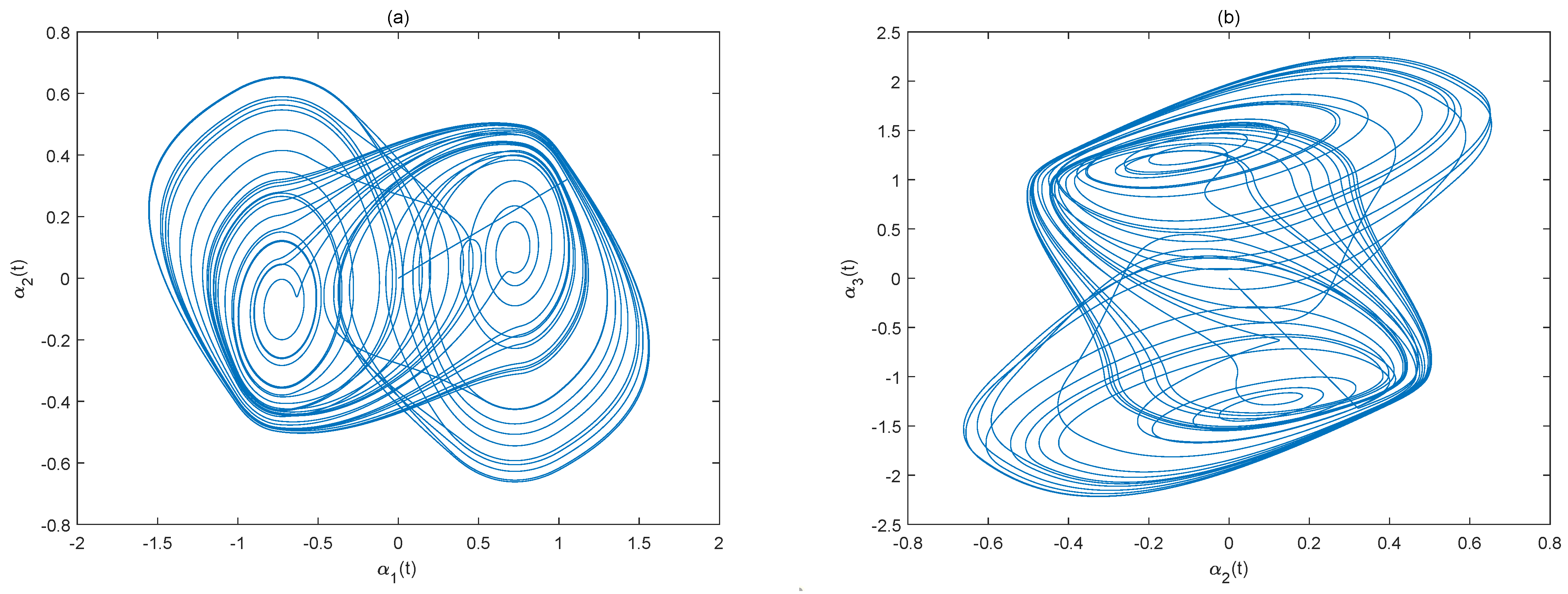
Figure 1.
Chaotic behavior of on (a) and (b) .


Figure 3.
Schematic of the saturated aperiodic sampled-data (SD) controller of Example I.

Figure 4.
Schematic of the master system and the slave system under the saturated aperiodic SD controller of Example I.
Figure 4.
Schematic of the master system and the slave system under the saturated aperiodic SD controller of Example I.

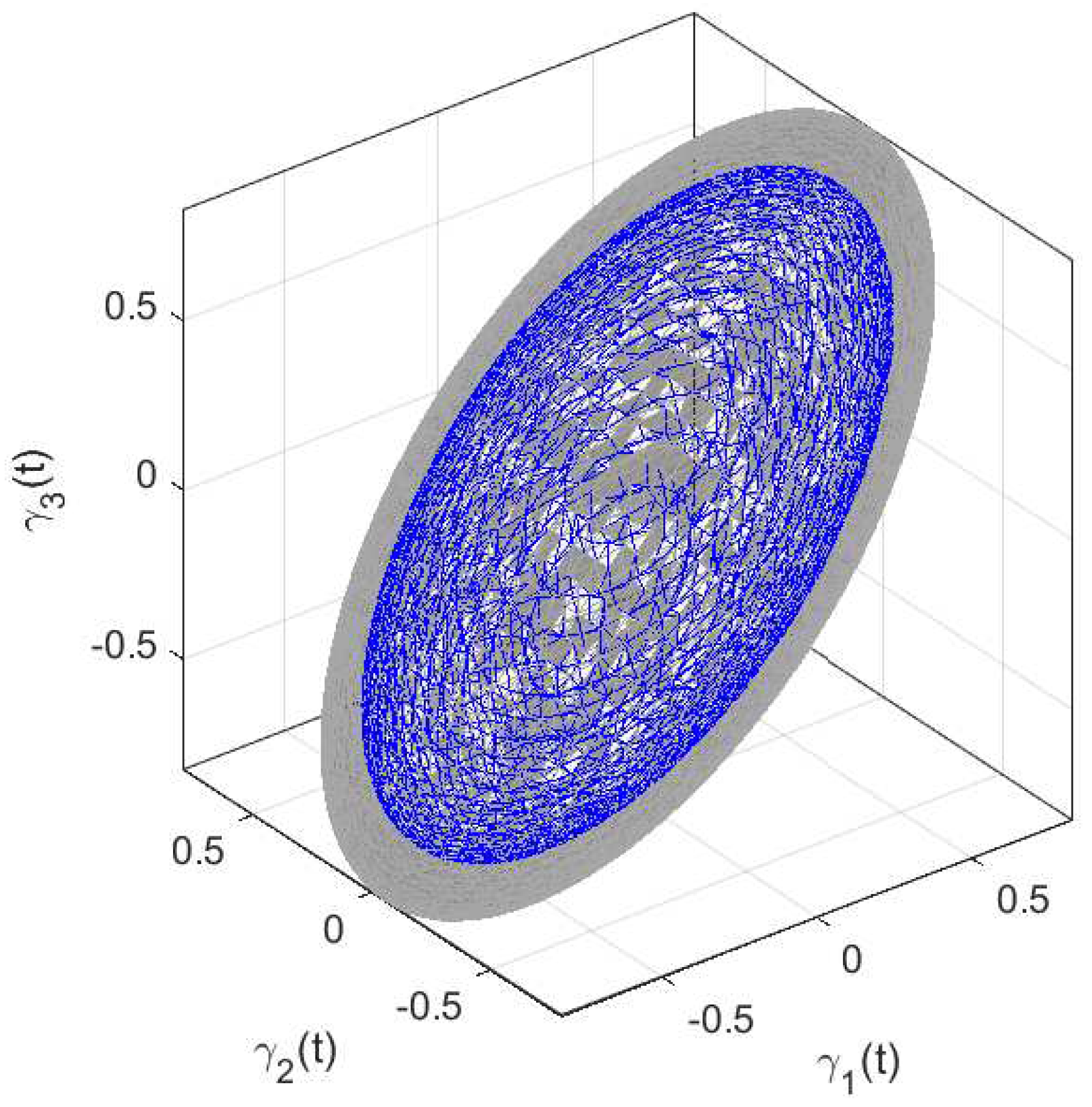
Figure 5.
Schematic of the error system under the saturated aperiodic SD controller of Example I.

Figure 6.
Schematic of the saturated aperiodic SD controller of Example II.

Figure 7.
Schematic of the master system and the slave system under the saturated aperiodic SD controller of Example II.
Figure 7.
Schematic of the master system and the slave system under the saturated aperiodic SD controller of Example II.

Figure 8.
Schematic of the error system under the saturated aperiodic SD controller of Example II.


Disclaimer/Publisher’s Note: The statements, opinions and data contained in all publications are solely those of the individual author(s) and contributor(s) and not of MDPI and/or the editor(s). MDPI and/or the editor(s) disclaim responsibility for any injury to people or property resulting from any ideas, methods, instructions or products referred to in the content. |
© 2023 by the authors. Licensee MDPI, Basel, Switzerland. This article is an open access article distributed under the terms and conditions of the Creative Commons Attribution (CC BY) license (https://creativecommons.org/licenses/by/4.0/).
Share and Cite
MDPI and ACS Style
Li, M.; Fan, Y. Aperiodic Sampled-Data Control for Anti-Synchronization of Chaotic Nonlinear Systems Subject to Input Saturation. Axioms 2023, 12, 403. https://doi.org/10.3390/axioms12040403
AMA Style
Li M, Fan Y. Aperiodic Sampled-Data Control for Anti-Synchronization of Chaotic Nonlinear Systems Subject to Input Saturation. Axioms. 2023; 12(4):403. https://doi.org/10.3390/axioms12040403
Chicago/Turabian StyleLi, Meixuan, and Yingjie Fan. 2023. "Aperiodic Sampled-Data Control for Anti-Synchronization of Chaotic Nonlinear Systems Subject to Input Saturation" Axioms 12, no. 4: 403. https://doi.org/10.3390/axioms12040403
Note that from the first issue of 2016, this journal uses article numbers instead of page numbers. See further details here.