
On the Fixed Circle Problem on Metric Spaces and Related Results


1
Department of Mathematics and Sciences, Prince Sultan University, Riyadh 11586, Saudi Arabia
2
Department of Mathematics, Izmir Democracy University, Izmir 35140, Turkey
3
Department of Mathematics, Balıkesir University, Balıkesir 10145, Turkey
*
Author to whom correspondence should be addressed.
Axioms 2023, 12(4), 401; https://doi.org/10.3390/axioms12040401
Submission received: 17 March 2023
/
Revised: 16 April 2023
/
Accepted: 18 April 2023
/
Published: 20 April 2023
(This article belongs to the Special Issue Fixed Point Theory and Its Related Topics IV)
Abstract
:The fixed-circle issue is a geometric technique that is connected to the study of geometric characteristics of certain points, and that are fixed by the self-mapping of either the metric space or of the generalized space. The fixed-disc problem is a natural resultant that arises as a direct outcome of this problem. In this study, our goal is to examine new classes of self-mappings that meet a new particular sort of contraction in a metric space. The common geometrical characteristic of the set of fixed points of any element of these classes is that a circle or even a disc, that is either termed the fixed circle or even the fixed disc of the appropriate self-map, is included within that set. In order to accomplish this, we establish two new classifications of contraction mapping: -contractive mapping and -expanding mapping. In the investigation of neural networks, activation functions with either fixed circles (or even fixed discs) are observed frequently. This demonstrates how successful our results with the fixed-circle (respectively, the fixed-disc) model were.
1. Introduction
Over the course of the past few decades, the Banach contraction principle has been researched and expanded upon using a variety of methods. These methods include generalizing the contractive condition that was utilized (see [1,2,3,4,5,6,7,8,9,10,11,12,13,14,15,16,17,18,19,20] for more details) and to generalize the used metric space (see [21,22,23,24,25,26,27,28,29] for more details). A recent approach is to examine the geometric characteristics of the fixed point set of a self-mapping with the help of a special geometric shape, introduced by Özgür and Taş in [30]. For this purpose, several theorems on the fixed circle are derived as the geometric aspects of the generalization of fixed-point theorems (see [30,31,32,33,34], for further information).
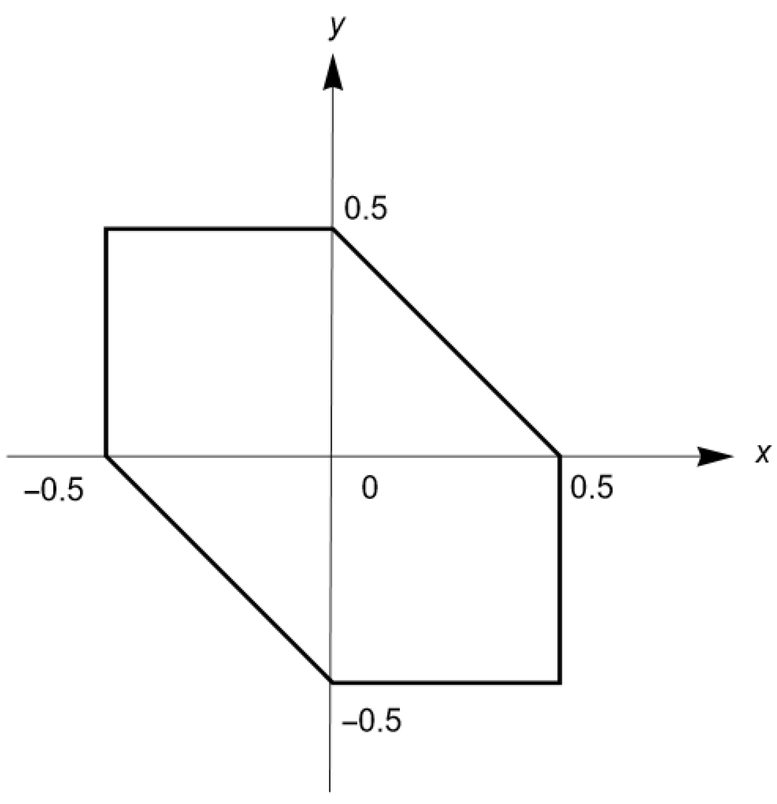
Consider the metric space and consider f as a self-mapping on . First, we recall that circle is a fixed circle of f if for all (see [30]). Similarly, disc is called a fixed disc of f if for all . There are several cases of self-mappings that demonstrate how the fixed point set of the self-mapping contains a circle (or a disc). Consider, for instance, the metric space along with the metric defined for the complex numbers and , as follows:
It is important to point out that the metric described in (1) is the same as the metric that is induced by the norm function
(notice the example given in 2.4 of [35]). In the accompanying illustration that was created with [36], you can see the circle denoted by . Define the self-mapping on , as follows:
for each , then clearly the fixed point set of contains circle , that is, is a fixed circle of (see Figure 1). Therefore, the study of geometrical properties of the fixed points of a self-mapping seems to be an intriguing problem in the case where the fixed point is non unique.
Moreover, self-mappings with fixed points are becoming more important to researchers studying neural networks. For instance, in [37], it was pointed out that the fixed points of a neural network can be determined by the fixed points of the activation function used. If the global input-output relationship in a neural network can be considered in the framework of Möbius transformations, then the existence of one or two fixed points throughout the neural network is guaranteed (see [38] for basic algebraic and geometric properties of Möbius transformations). Some possible applications of theoretical fixed-circle results to neural networks have been investigated in recent studies [30,32].
Next, we remind the readers of the following theorems on a fixed circle.
Theorem 1
([30]). Consider the metric space and let the mapping
for every . If there exists a self-mapping meeting
and
for every , hence circle is a fixed circle of f.
Theorem 2
Theorem 3
Theorem 4
([32]). Assume that is a metric space and the mapping be defined by
for every . If there exits a self-mapping meeting
- 1.
- for every ,
- 2.
- for every and ,
- 3.
- for every ,
hence circle is a fixed circle of f.
The following is the organization of this manuscript. In Section 2, we provide some generalizations of Theorems 1–3. In Section 3, we present the definitions of an “-contraction” and an “-expanding map” where we prove new theorems on a fixed circle. In Section 4, we consider the fixed point sets of some activation functions frequently used in the study of neural networks with a geometric viewpoint. This demonstrates how effective our results are, based on fixed circles. In Section 5, we present some open problems for future studies. When the fixed point we are looking at is not unique, our findings highlight the significance of the geometry of the other fixed points in a self-mapping.
2. New Fixed-Circle Theorems for Some Generalized Contractive Mappings
First, we provide a theorem for a fixed circle using an auxiliary function.
Theorem 5.
Assume that is a metric space, f is a self-mapping on Y and the mapping is described by
for every and . Suppose that
- 1.
- for some and every ,
- 2.
- for every ,
- 3.
- for every and ,
- 4.
- for every and ,
then, f fixes the circle .
Proof.
Let be a point chosen at random. By using conditions (1) and (2), we obtain
and so
There are two distinct cases.
Case 1. If , then we find by (4), that is, we have . Assume that for . Since , by using condition (3), we obtain
Furthermore, using condition (4)
and hence
which contradicts inequality (5). Therefore, it should be by which it implies that .
Case 2. Let . If , we obtain a contradiction by (4). Hence, it should be .
Thereby, we obtain for every , that is, is a fixed circle of f. To put it another way, the fixed point set of f contains circle . □
Remark 1.
Notice that, if we consider the case in condition of Theorem 5 for , then we obtain
and hence
For , we obtain
This means that condition (resp. condition is satisfied for this case.
Clearly, condition of Theorem 5 is the same as condition . Moreover, if condition of Theorem 5 is fulfilled, then condition is satisfied. Consequently, Theorem 5 is a generalization of Theorems 1 and 3 for the cases . For the case , Theorem 5 coincides with Theorem 1, and it is a particular case of Theorem 3.
Next, we present some illustrative examples.
Example 1.
Consider the metric space with the standard metric and circle . If we describe the self-mapping as
for each y belongs to , so it is not difficult to see that meets the hypothesis of Theorem 5 for circle and . Indeed, conditions (2), (3), and (4) of Theorem 5 can be easily checked. For condition (1), we take into consideration the two cases below.
Case 1. Let . Hence, we have and so
Case 2. Let . Then we have and hence, . Clearly, we have
Consequently, is the fixed circle of .
Example 2.
Consider to be the standard metric space and circle . Define by
for each , then does not meet condition of Theorem 5 for each and for any . Furthermore, does not fulfil condition for each and for any . Clearly, does not fix , and this example shows that condition is crucial in Theorem 5.
Example 3.
Consider to be the standard metric space and circles and . If we define as
for each , then meets the hypothesis of Theorem 5 for circles and and for any . Clearly, and are the fixed circles of .
Example 4.
Consider to be the standard metric space and describe the self-mapping as
for each . Hence, g meets both conditions and of Theorem 5; however, it does not meet condition for circle . However, the fixed point set of g consists of points and . So, circle is not a fixed circle of g, and this example shows that condition is required to obtain a fixed circle.
Moreover, is the unique fixed circle of g. It is simple to verify that g satisfies conditions and of Theorem 5, but does not satisfy condition for circle . This demonstrates that the conclusion reached by applying the opposite of Theorem 5 does not hold true in most situations. Again, condition is also crucial here.
We give another result of a fixed circle.
Theorem 6.
Let be a metric space, f be a self-mapping on Y and the mapping be, as in Theorem 5. Suppose that
- 1.
- for some and each ,
- 2.
- for each ,
- 3.
- for every and ,
- 4.
- for each and ,
hence, circle is fixed by the self-mapping f.
Proof.
Consider to be an arbitrary point. Using conditions (1) and (2), we obtain
and
Similar to the arguments used in the proof of Theorem 5, a direct computation indicates that circle is fixed by f. □
Remark 2.
Notice that, if we consider the case in condition of Theorem 6 for , then we obtain
Hence, condition is satisfied. Furthermore, condition of Theorem 6 is contained in condition . Therefore, Theorem 6 is a particular case of Theorem 2 in this case. For the cases , Theorem 6 is an extension of Theorem 2.
Now, we look at some instances to help illustrate our point.
Example 5.
Consider the standard metric space and circle . Consider the map as
for each , hence, satisfies the hypothesis of Theorem 6 for . Clearly, is a fixed circle of . It is easy to check that does not fulfill condition of Theorem 5 to any .
Example 6.
Consider the standard metric space and circles and . Consider the self-mapping defined by
for each and , so satisfies the hypothesis of Theorem 6 for and for circles and . Clearly, and are the fixed circles of . Notice that fixed circles and are not disjoint.
Considering Examples 3 and 6, we deduce that a fixed circle does not require the uniqueness in Theorems 5 and 6. If a fixed circle is non unique, then two fixed circles of a self-mapping can be disjoint or not. Next, we prove a theorem where f fixes a unique circle.
Theorem 7.
Let be a metric space and be a self-mapping that fixes circle . If the following condition
is satisfied by f for every and , then is the unique fixed circle of f.
Proof.
Let be another fixed circle of f. If we take and with , from the inequality (7), we obtain
that is a contradiction. We have for every , then f has only one fixed circle □
Example 7.
Consider the standard metric space and circle Define on as follows:
for , where represents the complex conjugate of t. It is not difficult to see that is the unique fixed circle of , where does not fulfil the hypothesis of Theorem 7.
Example 7 demonstrates that the counterfactual of Theorem 7 is not correct in general. Now, in order to illustrate Theorem 7, we consider the following example.
Example 8.
Let and the metric be described by
for every . If we take the self-mapping is described by
for any ; hence, is the unique fixed circle of
Next, we present the following interesting theorem that involves the identity map described by for all
Theorem 8.
Consider the metric space . Let the map f be from to itself with fixed circle . The self-mapping f fulfils the following condition
for every and some , if and only when .
Proof.
Take with . By inequality (8), if , then we obtain
which leads us to a contradiction due to the fact that . If , then we obtain
Hence, we have and that is , since y is an arbitrary point in .
Conversely, satisfies condition (8) clearly. □
Corollary 1.
Let be a metric space and be a self-mapping. If f satisfies the hypothesis of Theorem 5 (resp. Theorem 6) but condition (8) is not satisfied, then .
Now, we rewrite the next theorem given in [30].
Theorem 9
Theorem 10.
Proof.
The proof follows easily. □
3. New Classes of Contractive and Expanding Mappings in Metric Spaces
In this part of the article, we will apply a different strategy to acquire new results for the fixed circle. This new approach also ensures the existence of a fixed disc of a self-mapping. The following group of functions, which was first presented by Wardowski in [39], is our primary resource for accomplishing this.
Definition 1
([39]). Let stand for the entire group of functions in such a way that
is neither decreasing nor constant,
For every sequence in the below must be true.
There exists such that .
Several examples of functions that satisfy the axioms , and of Definition 1 are the following , , and (check [39] for further information).
At this point, we are going to discuss a new sort of contraction that goes as follows.
Definition 2.
Consider the metric space . Let f be a self-mapping on . If there exists , and in such a way that
for every , then f is called as an -contraction.
It is important to notice that the point , which is referred to in Definition 2, needs to be a fixed point in the mapping f. In fact, if is not a fixed point of f, we obtain and then
It is clear that it is a contradiction due to the fact that the domain of is . As a result, the next proposition may be stated as a direct consequence of Definition 2.
Proposition 1.
Consider the metric space . If f is an -contraction with , then we obtain .
Using this new type of contraction, we will now state the following fixed-circle theorem.
Theorem 11.
Consider the metric space . Let f be an -contraction with . Define the number γ by
Then, is a fixed circle of f. Particularly, f fixes each circle where .
Proof.
If , then clearly , and by using Proposition 1, we observe that is a fixed circle of f. Assume and let . If , then by the definition of , we have . Since is increasing, using the -contractive property of f, we obtain
which leads to a contradiction. Therefore, we have , that is, . Consequently, is a fixed circle of f.
Now, we prove that f also fixes any arbitrary circle with . Take and assume that . Again, using the -contractive property of the self-mapping, we obtain
Since is increasing, we find
However, , which brings forth a contradiction. Hence, we obtain , that is, . Accordingly, , is a circle of f that is fixed. □
Remark 3.
(1) We note that in Theorem 11, the -contraction f fixes the disc . Hence, the centre of any fixed circle is also fixed by f. In Theorem 4, the self-mapping f maps into (or onto) itself, but the centre of the fixed circle does not require to be fixed by f.
(2) In relation to the number of points in the set , the number of fixed circles of an -contractive self-mapping f may be infinite (see Example 11).
We give some illustrative examples.
Example 9.
We consider the set with the usual metric and identify the self-mapping as
The self-mapping is an -contractive self-mapping, such as , and . Obviously, we have only for the point and
Clearly, we obtain , and fixes the circle . fixes also the disc . Notice that circle is another fixed circle of .
As may be observed in the following illustration, the converse assertion of Theorem 11 does not always hold true.
Example 10.
Take as a metric space, be any arbitrary point and be any number. If we consider the self-mapping defined by
Therefore, it is not hard to realize that is not an -contractive self-mapping for the point but fixes each circle where .
Example 11.
Consider the standard metric space and describe the self-mapping as
for all . We have and is an -contractive self-mapping with , and . Clearly, the self-mapping has infinitely many circles that are fixed.
Presently, we have settled on a new theorem of fixed circles based on the following well-known fact, that if a self-mapping f on is surjective, then there exists a self mapping , in such a way that the map is the identity map for . First, we give a new type of expanding map.
Definition 3.
A self-mapping f on a metric space is referred to as an -expanding map, if there exist , and in such a way that
for every .
Theorem 12.
Consider the metric space . If is a surjective -expanding map with , then f has a circle that is fixed in
Proof.
Since f is surjective, there exists a self-mapping such that the map is the identity map for . Take be such that and . First, notice the following fact
Since
by using -expanding property of f, we obtain
and
Therefore, we obtain
Consequently, is an -contraction of with as . Then, using Theorem 11, has a fixed circle . Let be any point. Using the fact that
we deduce that , then z is a fixed point of f, which implies that f also fixes , as required. □
Example 12.
Let us take the set with the standard metric and define the self-mapping by
is a surjective -expanding map with , and . We obtain
and circle is the fixed circle of f.
Example 13.
Let be the standard metric space and consider the self-mapping defined by
for all . We have
is a surjective -expanding map with , and . Indeed, we obtain
for each z with . Circle is a fixed circle of f.
Remark 4.
The conclusion for Theorem 12 does not hold true in all cases if f is not a surjective map. For instance, if we consider the set using the standard metric and let the self-mapping be defined as where
It is not hard to verify that fulfils the condition
for all , with , and . Therefore, meets all of the axioms of Theorem 12, except that is not surjective. Notice that and does not fix circle .
4. Fixed Point Sets of Activation Functions
Activation functions are the primary neural networks’ decision-making units in a neural network; and hence, it is important to choose the most appropriate activation function for the neural network analysis [40,41]. Characteristic properties of activation functions play an important role in learning and stability issues of a neural network. A comprehensive analysis of different activation functions with individual real-world applications was given in [40]. We note that the fixed point sets of commonly used activation functions (e.g., Ramp function, ReLU function, Leaky ReLU function) contain some fixed discs and fixed circles.
Example 14.
Let us consider the Leaky ReLU function defined by
where . In [42], the Leaky–Reluplex algorithm was proposed to verify deep neural networks (DNNs) with the Leaky ReLU activation function (see [42] for more details). Now, we consider the fixed point set of the Leaky ReLU activation function by a geometric viewpoint. Clearly, the fixed point set of f is . Let be a fixed point and consider the circle . Then, it is easy to verify that the function meets the criteria of Theorem 5 for circle with . Clearly, circle is a fixed circle of f and the centre of the fixed circle is also fixed by f.
Most of the known fixed point theorems (e.g., Banach fixed point theorem, Brouwer’s fixed point theorem) have been used in the theoretic studies of neural networks. For example, in [43], the existence of a fixed point for every recurrent neural network was shown, and a geometric approach was used to locate the fixed points. Brouwer’s fixed point theorem was used to maintain the existence of a fixed point. This study shows the importance of the geometric viewpoint and theoretic fixed point results in applications.
5. Conclusions and Prospective Initiatives
In this section, we point out the investigation of some open questions. Concerning the geometry of non unique fixed points of a self-mapping on a metric space, novel geometric (fixed-circle or fixed-disc) findings have been found. To do this, we use two different approaches. One of them is to measure whether a given circle is fixed or not by a self-mapping. Another approach is to find which circle is fixed by a self-mapping under some contractive or expanding conditions. The investigation of new conditions which ensure that a circle or a disc is fixed by a self-mapping can be considered as a future problem. For a self-mapping in which the fixed point set contains a circle or a disc, new contractive or expanding conditions can also be investigated.
Additionally, there are several examples of self-mappings that have a common fixed circle. Here is an example, let be the usual metric space and consider circle . We define the self-mappings and by
for each , respectively. Both self-mappings and fix circle , then, circle is a common fixed circle of the self-mappings and . At this point, the following question can be left for future study.
Question 13.
What condition(s) must exist for any circle to be the common fixed circle for two or more self-mappings?
In conclusion, the problems discussed in this study can also be investigated on various generalized metric spaces. For instance, the notion of an -metric space was introduced in [44].
Notation 14.
We use the following notations.
- 1.
- 2.
Definition 4.
An -metric on a set that contains at least one point is function , if for all we have
- 1.
- 2.
- 3.
- 4.
- Then, the pair is called an -metric space.
One can consult [44] for some examples and basic notions of an -metric space.
In -metric spaces, we define a circle as follows:
Question 15.
Consider the -metric space where , and let f be a surjective self-mapping on . Yet, we obtain
for every and some . Does f have a point circle on
Question 16.
Let be an -metric space, , , and f be a surjective self-mapping on . Yet, we have
for every and some . Does f have a fixed circle on
Author Contributions
N.M.: supervision, writing—original draft, methodology; N.Ö.: conceptualization, writing—original draft; N.T.: conceptualization, writing—original draft; D.S.: conceptualization, writing—original draft. All authors have read and agreed to the published version of the manuscript.
Funding
This research received no external funding.
Data Availability Statement
Not applicable.
Acknowledgments
The authors thank to the referees for valuable comments and remarks which improved the original manuscript. The authors N. Mlaiki and D. Santina would like to thank Prince Sultan University for funding this work through TAS LAB.
Conflicts of Interest
The authors declare no conflict of interest.
References
- Altun, I.; Aslantaş, M.; Şahin, H. Best proximity point results for p-proximal contractions. Acta Math. Hung. 2020, 162, 393–402. [Google Scholar] [CrossRef]
- Caristi, J. Fixed point theorems for mappings satisfying inwardness conditions. Trans. Am. Math. Soc. 1976, 215, 241–251. [Google Scholar] [CrossRef]
- Chatterjea, S.K. Fixed point theorem. C. R. Acad. Bulgare Sci. 1972, 25, 727–730. [Google Scholar] [CrossRef]
- Ćirić, L.B. A generalization of Banach’s contraction principle. Proc. Am. Math. Soc. 1974, 45, 267–273. [Google Scholar] [CrossRef]
- Djafari Rouhani, B.; Moradi, S. On the existence and approximation of fixed points for Ćirić type contractive mappings. Quaest. Math. 2014, 37, 179–189. [Google Scholar] [CrossRef]
- Edelstein, M. On fixed and periodic points under contractive mappings. J. Lond. Math. Soc. 1962, 37, 74–79. [Google Scholar] [CrossRef]
- Kannan, R. Some results on fixed points II. Am. Math. Mon. 1969, 76, 405–408. [Google Scholar]
- Kim, H. Fixed point theorems for Chandrabhan type maps in abstract convex uniform spaces. J. Nonlinear Funct. Anal. 2021, 2021, 1–8. [Google Scholar]
- Latif, A.; Al Subaie, R.F.; Alansari, M.O. Fixed points of generalized multi-valued contractive mappings in metric type spaces. J. Nonlinear Var. Anal. 2022, 6, 123–138. [Google Scholar]
- Nemytskii, V.V. The fixed point method in analysis. Usp. Mat. Nauk 1936, 1, 141–174. (In Russian) [Google Scholar]
- Olgun, M.; Biçer, Ö.; Alyıldız, T.; Altun, İ. A related fixed point theorem for F-contractions on two metric spaces. Hacet. J. Math. Stat. 2019, 48, 150–156. [Google Scholar] [CrossRef]
- Rhoades, B.E. A comparison of various definitions of contractive mappings. Trans. Amer. Math. Soc. 1977, 226, 257–290. [Google Scholar] [CrossRef]
- Shatanawi, W. On w-compatible mappings and common coupled coincidence point in cone metric spaces. Appl. Math. Lett. 2012, 25, 925–931. [Google Scholar] [CrossRef]
- Shatanawi, W.; Ćojbašić Rajić, R.V.; Radenović, S.; Al-Rawashdeh, A. Mizoguchi-Takahashi-type theorems in tvs-cone metric spaces. Fixed Point Theory Appl. 2012, 106, 7. [Google Scholar] [CrossRef]
- Al-Rawashdeh, A.; Aydi, H.; Felhi, A.; Sehmim, S.; Shatanawi, W. On common fixed points for α-F-contractions and applications. J. Nonlinear Sci. Appl. 2016, 9, 3445–3458. [Google Scholar] [CrossRef]
- Shatanawi, W.; Mustafa, Z.; Tahat, N. Some coincidence point theorems for nonlinear contraction in ordered metric spaces. Fixed Point Theory Appl. 2011, 68, 15. [Google Scholar] [CrossRef]
- Shatanawi, W. Some fixed point results for generalized ψ-weak contraction mappings in orbitally metric spaces. Chaos Solitons Fractals 2012, 45, 520–526. [Google Scholar] [CrossRef]
- Shatanawi, W.; Shatnawi, T.A.M. New fixed point results in controlled metric type spaces based on new contractive conditions. AIMS Math. 2023, 8, 9314–9330. [Google Scholar] [CrossRef]
- Rezazgui, A.-Z.; Tallafha, A.A.; Shatanawi, W. Common fixed point results via Aν—α—contractions with a pair and two pairs of self-mappings in the frame of an extended quasi b-metric space. AIMS Math. 2023, 8, 7225–7241. [Google Scholar] [CrossRef]
- Joshi, M.; Tomar, A.; Abdeljawad, T. On fixed points, their geometry and application to satellite web coupling problem in S—metric spaces. AIMS Math. 2023, 8, 4407–4441. [Google Scholar] [CrossRef]
- An, T.V.; Dung, N.V.; Kadelburg, Z.; Radenović, S. Various generalizations of metric spaces and fixed point theorems. Rev. R. Acad. Cienc. Exactas Fis. Nat. Ser. A Math. 2015, 109, 175–198. [Google Scholar] [CrossRef]
- Bakhtin, I.A. The contraction mapping principle in almost metric spaces. Funct. Anal. Gos. Ped. Inst. Unianowsk 1989, 30, 26–37. [Google Scholar]
- Gähler, S. 2-metrische Räume und ihre topologische Struktur. Math. Nachr. 1963, 26, 115–148. [Google Scholar] [CrossRef]
- Karayılan, H.; Telci, M. Caristi type fixed point theorems in fuzzy metric spaces. Hacet. J. Math. Stat. 2019, 48, 75–86. [Google Scholar] [CrossRef]
- Mustafa, Z.; Sims, B. A new approach to generalized metric spaces. J. Nonlinear Convex Anal. 2006, 7, 289–297. [Google Scholar]
- Mitrović, Z.D.; Radenović, S. A common fixed point theorem of Jungck in rectangular b-metric spaces. Acta Math. Hung. 2017, 153, 401–407. [Google Scholar] [CrossRef]
- Pasicki, L. A strong fixed point theorem. Topol. Appl. 2020, 282, 107300. [Google Scholar] [CrossRef]
- Sedghi, S.; Shobe, N.; Aliouche, A. A generalization of fixed point theorems in S-metric spaces. Mat. Vesn. 2012, 64, 258–266. [Google Scholar]
- Sihag, V.; Vats, R.K.; Vetro, C. A fixed point theorem in G-metric spaces via α-series. Quaest. Math. 2014, 37, 429–434. [Google Scholar] [CrossRef]
- Özgür, N.Y.; Taş, N. Some fixed-circle theorems on metric spaces. Bull. Malays. Math. Sci. Soc. 2019, 42, 1433–1449. [Google Scholar] [CrossRef]
- Özgür, N.Y.; Taş, N. Fixed-circle problem on S-metric spaces with a geometric viewpoint. Facta Univ. Ser. Math. Inform. 2019, 34, 459–472. [Google Scholar] [CrossRef]
- Özgür, N.Y.; Taş, N. Some fixed-circle theorems and discontinuity at fixed circle. AIP Conf. 2018, 1926, 020048. [Google Scholar]
- Özgür, N.Y.; Taş, N.; Çelik, U. New fixed-circle results on S-metric spaces. Bull. Math. Anal. Appl. 2017, 9, 10–23. [Google Scholar]
- Özgür, N. Fixed-disc results via simulation functions. Turk. J. Math. 2019, 43, 2794–2805. [Google Scholar] [CrossRef]
- Özgür, N.Y. Ellipses and similarity transformations with norm functions. Turk. J. Math. 2018, 42, 3204–3210. [Google Scholar] [CrossRef]
- Wolfram Research, Inc. Mathematica; Version 12.0; Wolfram Research, Inc.: Champaign, IL, USA, 2019. [Google Scholar]
- Mandic, D.P. The use of Möbius transformations in neural networks and signal processing. In Neural Networks for Signal Processing X, Proceedings of the 2000 IEEE Signal Processing Society Workshop (Cat. No. 00TH8501), Sydney, Australia, 11–13 December 2000; IEEE: Piscataway, NJ, USA; Volume 1, pp. 185–194.
- Jones, G.A.; Singerman, D. Complex Functions: An Algebraic and Geometric Viewpoint; Cambridge University Press: Cambridge, UK, 1987. [Google Scholar]
- Wardowski, D. Fixed points of a new type of contractive mappings in complete metric spaces. Fixed Point Theory Appl. 2012, 2012, 94. [Google Scholar] [CrossRef]
- Szandała, T. Review and Comparison of Commonly Used Activation Functions for Deep Neural Networks, In Bio-Inspired Neurocomputing. Studies in Computational Intelligence; Bhoi, A., Mallick, P., Liu, C.M., Balas, V., Eds.; Springer: Singapore, 2021; Volume 903. [Google Scholar] [CrossRef]
- Zhang, L. Implementation of fixed-point neuron models with threshold, ramp and sigmoid activation functions. IOP Conf. Ser. Mater. Sci. Eng. 2017, 224, 012054. [Google Scholar] [CrossRef]
- Xu, J.; Li, Z.; Du, B.; Zhang, M.; Liu, J. Reluplex made more practical: Leaky ReLU. In Proceedings of the 2020 IEEE Symposium on Computers and Communications (ISCC), Rennes, France, 7–10 July 2020; IEEE: Piscataway, NJ, USA, 2020; pp. 1–7. [Google Scholar]
- Li, L.K. Fixed point analysis for discrete-time recurrent neural networks. In Proceedings of the 1992 IJCNN International Joint Conference on Neural Networks, Baltimore, MD, USA, 15–19 January 1992; Volume 4, pp. 134–139. [Google Scholar]
- Mlaiki, N.; Souayah, N.; Abodayeh, K.; Abdeljawad, T. Contraction principles in Ms—metric spaces. J. Nonlinear Sci. Appl. 2017, 10, 575–582. [Google Scholar] [CrossRef]
Figure 1.
The graph of the circle .

Disclaimer/Publisher’s Note: The statements, opinions and data contained in all publications are solely those of the individual author(s) and contributor(s) and not of MDPI and/or the editor(s). MDPI and/or the editor(s) disclaim responsibility for any injury to people or property resulting from any ideas, methods, instructions or products referred to in the content. |
© 2023 by the authors. Licensee MDPI, Basel, Switzerland. This article is an open access article distributed under the terms and conditions of the Creative Commons Attribution (CC BY) license (https://creativecommons.org/licenses/by/4.0/).
Share and Cite
MDPI and ACS Style
Mlaiki, N.; Özgür, N.; Taş, N.; Santina, D. On the Fixed Circle Problem on Metric Spaces and Related Results. Axioms 2023, 12, 401. https://doi.org/10.3390/axioms12040401
AMA Style
Mlaiki N, Özgür N, Taş N, Santina D. On the Fixed Circle Problem on Metric Spaces and Related Results. Axioms. 2023; 12(4):401. https://doi.org/10.3390/axioms12040401
Chicago/Turabian StyleMlaiki, Nabil, Nihal Özgür, Nihal Taş, and Dania Santina. 2023. "On the Fixed Circle Problem on Metric Spaces and Related Results" Axioms 12, no. 4: 401. https://doi.org/10.3390/axioms12040401
Note that from the first issue of 2016, this journal uses article numbers instead of page numbers. See further details here.