Reconstructing Loads in Nanoplates from Dynamic Data

Abstract

It was recently proved that the knowledge of the transverse displacement of a nanoplate in an open subset of its mid-plane, measured for any interval of time, allows for the unique determination of the spatial components ${\left\{f_m(x,y)\right\}}_{m=1}^M$ of the transverse load ${\sum }_{m=1}^M{g}_m\left(t\right)f_m(x,y)$, where $M\ge 1$ and ${\left\{g_m\left(t\right)\right\}}_{m=1}^M$ is a known set of linearly independent functions of the time variable. The nanoplate mechanical model is built within the strain gradient linear elasticity theory, according to the Kirchhoff–Love kinematic assumptions. In this paper, we derive a reconstruction algorithm for the above inverse source problem, and we implement a numerical procedure based on a finite element spatial discretization to approximate the loads ${\left\{f_m(x,y)\right\}}_{m=1}^M$. The computations are developed for a uniform rectangular nanoplate clamped at the boundary. The sensitivity of the results with respect to the main parameters that influence the identification is analyzed in detail. The adoption of a regularization scheme based on the singular value decomposition turns out to be decisive for the accuracy and stability of the reconstruction.

1. Introduction

In this paper, we report the results of a systematic numerical study—the first one published in the literature, to our knowledge—on the identification of transverse pressures exerted on a nanoplate from the measurement of its transverse vibrational response in an open subset of the mid-plane, for any interval of time. From the mathematical point of view, the small transverse vibration $u=u(t,x,y)$ of a clamped nanoplate, with constant thickness and mid-plane $\Omega$, made by homogeneous and linearly elastic isotropic material is governed by the following boundary value problem with initial data [1]:

$$\{\begin{array}{lll}{\rho }_0{u}_{,tt}+p_2{\Delta }^{2}u-p_1{\Delta }^{3}u=F(t,x,y),\hfill & \mathrm{in} ]0,\mathcal{T}[\times \Omega ,\hfill & \hfill \left(1\right)\\ u=u_{,m}=u,nn=0,\hfill & \mathrm{on} ]0,\mathcal{T}[\times \partial \Omega ,\hfill & \hfill \left(2\right)\\ u=u_{,t}=0,\hfill & \mathrm{at} \{t=0\}\times \Omega .\hfill & \hfill \left(3\right)\end{array}$$

In the above equation, $F=F(t,x,y)$ is the transverse force per unit area; ${\rho }_0$ is the constant mass density per unit area; $p_1$ and $p_2$ are two (positive) stiffness coefficients taking into account the two classical Lamé moduli, the thickness of the plate, and the three material length scale parameters of the simplified strain gradient elasticity theory by Lam et al. [2] within the Kirchhoff–Love kinematic framework (see Section 2.1 for details). We refer to [3] for an updated review of the state-of-the-art size-dependent continuum models of plates.

Determining the forcing term F from time-history measurements of the nanoplate deformation is of interest in several technological areas. Applications generally involve nanoplates used as sensors and may concern, for example, the early sensing of pressures induced by shock waves either produced by explosions or strong chemical reactions in an inaccessible environment [4,5], the detection of forces of small magnitude such as chemical bonding and Van der Waals [6], or even the detection of weak variations of intraocular pressures [7].

A first general result for this class of inverse problems was recently obtained in [1] for the forcing term of the form $F={\sum }_{m=1}^M{g}_m\left(t\right)f_m(x,y)$, where $M\ge 1$ is a finite integer number. Under the assumption that the time-dependent functions ${\left\{g_m\left(t\right)\right\}}_{m=1}^M$ are known in an interval $[0,T_0]$, with $T_0>0$ arbitrarily small, and are linearly independent in any interval $I\subset ]0,\mathcal{T}[$, it was proved in [1] that the knowledge of the transverse displacement u in an open subset $\omega$ of the mid-plane $\Omega$ for any interval of time is enough for the unique determination of the spatial components ${\left\{f_m(x,y)\right\}}_{m=1}^M$ of the load.

It is worth mentioning that a rather extensive literature is available on the determination of loads from dynamic measurements acting on two-dimensional mechanical models [8,9,10,11,12]. The published results mainly concern the small transverse motions of taut membranes and classical Kirchhoff–Love plates, respectively governed by second-order (Laplacian, in the case of constant coefficients) and fourth-order (bilaplacian) spatial differential operators. Without claim of completeness and restricting the attention to the use of interior measurements on plates only, we mention the papers [13,14] that deal with rectangular plates. In them, it is proved that the spatial part $f\left(x\right)$ of loads of the form $g\left(t\right)f\left(x\right)$ can be uniquely identified when the temporal function $g\left(t\right)$ is known and the transverse deflection of the plate is measured along a line parallel to one of the sides stretching from side to side for an arbitrary small interval of time, provided the line is well positioned, or if the observation line does not stretch from side to side, the observation time interval is long enough. For mid-plane $\Omega$ of more general shapes, Kim [15] proved a unique continuation property for plates with smooth boundary $\partial \Omega$, when the data are obtained over an open set that contains $\partial \Omega$. The mathematical tools used in these papers were different from the one employed in [1], in which the idea of spherical means of the transverse displacement was applied.

The proof of the uniqueness result presented in [1] suggests a constructive procedure for determining the spatial component of the forcing term acting on a nanoplate. The main objective of this paper is the development and the numerical implementation of this reconstruction technique. The guiding idea is illustrated in Section 3. In short, it is based on the approximation of the spatial components $f_m(x,y)$, $m=1,\dots ,M$, with their truncated Fourier representation based on the eigenfunctions of the nanoplate, and on the determination of the generalized coefficients of the corresponding Fourier series from the measured transverse deflection of the nanoplate.

Section 4 shows the results of a selected collection of numerical simulations for a nanoplate with rectangular domain $\Omega$ and clamped boundary. They represent the outcomes obtained from a larger set of simulations. In the numerical analysis, we have examined in detail the effect of the main parameters that influence the identification, namely the typical size of the finite element mesh, the extent and position of the measurement subdomain $\tilde{\Omega }$, the number of terms used in the truncated series representation of the loads, and the reduction to a regularization scheme based on the Singular Value Decomposition. Overall, the results are encouraging and, among other things, show that the use of regularization is decisive in ensuring sufficient accuracy and stability of the identification, especially in the presence of multiple asynchronous loads ($M\ge 2$).

2. Nanoplate Model and FE Validation

In this section, we introduce a mechanical nanoplate model and its discrete version, which will be used to study the inverse problem of identifying spatial transverse forces from dynamic data.

2.1. A Strain-Gradient Elastic Nanoplate Model

Let us consider a nanoplate in the referential configuration $\Omega \times [-h/2,h/2]$, where $\Omega$ is an open, bounded, and connected subset of the plane representing the middle surface of the nanoplate, and h is the uniform thickness, $h<<diam(\Omega )$. In this sub-section, we assume that the boundary $\partial \Omega$ of $\Omega$ is smooth. Domains $\Omega$ with piecewise smooth boundaries (e.g., rectangular domains) will be considered later on.

We shall adopt the simplified strain gradient elasticity theory proposed by Lam et al. [2] to model the mechanical behavior of the material in infinitesimal deformation. In this simplified theory, for linear elastic center-symmetric isotropic materials, the number of independent length scale parameters is reduced from five (as in the general Mindlin’s theory [16]) to three; see also the recent paper by Munch et al. [17]. In particular, to simplify the presentation and in view of the reconstruction results presented in the next sections, we assume that the material is homogeneous, i.e., the elastic coefficients of the nanoplate are constant in space and time.

Under the kinematic assumptions of Kirchhoff–Love’s plate theory and assuming clamped boundary conditions, the boundary value problem with initial data governing the transverse displacement $u=u(t,x,y)$ of the mid-plane of the nanoplate reads as (see, for example, [1])

$$\{\begin{array}{lll}{\rho }_0{u}_{,tt}+p_2{\Delta }^{2}u-p_1{\Delta }^{3}u={\displaystyle \sum _{m=1}^M{g}_m}{f}_m,\hfill & \mathrm{in} ]0,\mathcal{T}[\times \Omega ,\hfill & \left(4\right)\\ u=u_{,n}=u_{,nn}=0,\hfill & \mathrm{on} ]0,\mathcal{T}[\times \partial \Omega ,\hfill & \left(5\right)\\ u=u_{,t}=0,\hfill & \mathrm{at} \{t=0\}\times \Omega ,\hfill & \left(6\right)\end{array}$$

where t is the time variable, $\mathcal{T}>0$, ${(·)}_{,t}=\partial (·)/\partial t$, and $\Delta$ is the Laplacian operator. The directional derivative of u along the outer unit normal $\mathbf{n}$ to $\Omega$ is denoted by $u{,}_n$.

In Equation (4), the area mass density of the nanoplate is denoted by ${\rho }_0$, ${\rho }_0=constant>0$, and the quantities $p_1$, $p_2$ are given by

$$p_1=\mu I(2{\ell }_0^2+\frac{4}{5}{\ell }_1^2),p_2=\mu h(2{\ell }_0^2+\frac{8}{15}{\ell }_1^2+{\ell }_2^2)+\frac{EI}{1-{\nu }^2},$$

(7)

where $I=\frac{h^3}{12}$, $\mu >0$ is the elastic shear modulus, $E>0$ is Young’s modulus, $\nu \in (0,1/2)$ is the Poisson’s coefficient of the material, and the (constant, positive) length scale parameters are denoted by ${\ell }_0$, ${\ell }_1$, ${\ell }_2$. Finally, note that, by (6), the nanoplate is assumed to be at rest at the initial time $t=0$.

The functions $f_m=f_m(x,y)$, $m\in \{1,\dots M\}$, describe the spatial component of the transverse forces acting over the plate, whereas the functions $g_m=g_m\left(t\right)$, $g_m\in {\mathcal{C}}^1\left(\right[0,\mathcal{T}\left[\right)$, for $m\in \{1,\dots ,M\}$, describe the temporal evolution of the loading.

The solution $u=u(x,y,t)$ of the forced motion problem (4)–(6) can be represented in a series of eigenfunctions $S=S(x,y)$ of the clamped nanoplate. These eigenfunctions are the (non-trivial) solutions $S\in \mathcal{P}=H^6(\Omega )\cap H_0^3(\Omega )$ to the boundary value problem

$$\{\begin{array}{ll}{\tilde{p}}_2{\Delta }^{2}S-{\tilde{p}}_1{\Delta }^{3}S={\lambda }^{2}S,\hspace{1em} \mathrm{in} \Omega ,\hfill & \left(8\right)\\ S=S_{,n}=S_{,nn}=0,\hspace{1em} \mathrm{on} \partial \Omega ,\hfill & \left(9\right)\end{array}$$

where we have defined ${\tilde{p}}_i=p_i/{\rho }_0$, $i=1,2$.

By general results for self-adjoint operators, there exists a sequence ${\left\{{\lambda }_i^2\right\}}_{i=1}^{\infty }$ of real numbers ${\lambda }_i^2>0$ (counted with repeated values according to their multiplicity), with ${lim}_{i\to +\infty }{\lambda }_i^2=+\infty$, such that $\{({\lambda }_i^2,S_i)\in {\mathbb{R}}_{+}\times \mathcal{P}\}$ is a non-trivial solution to (8) and (9) for every $i\ge 1$. Moreover, the family ${\left\{S_i\right\}}_{i=1}^{\infty }$, with $S_i$ enumerated with repeated values according to the multiplicity of the eigenvalues, is a complete Hilbertian basis of the space $\mathcal{P}$, and the eigenfunctions satisfy the orthogonality conditions ${(S_i,S_j)}_{L^2(\Omega )}={\delta }_{ij}/{\lambda }_i^2$, $i,j\ge 1$, where we have defined ${(h_1,h_2)}_{L^2(\Omega )}={\int }_{\Omega }{h}_1{h}_{2}d\Omega$ for every $h_1,h_2\in L^2(\Omega )$, and ${\delta }_{ij}$ is the Kronecker delta.

Let us assume that the spatial load distributions $f_m=f_m(x,y)$ belong to the dual of the space $\mathcal{P}$, $f_m\in {\mathcal{P}}^{\prime }$, for every $m=\{1,\dots ,M\}$. Therefore, if we represent $f_m$ as $\frac{f_m}{{\rho }_0}={\sum }_{k=1}^{+\infty }{\alpha }_{m,k}{\lambda }_k^2{S}_k$, for ${\left({\alpha }_{m,k}\right)}_{k\in \mathbb{N}}\in {\ell }^2$, then the unique solution $u\in {\mathcal{C}}^{}\left(\right[0,\mathcal{T}[,\mathcal{P})$ to the forced motion problem (4)–(6) can be expressed as

$$u(t,x,y)=\sum _{m=1}^M{\int }_0^t{g}_m(t-\tau )\sum _{k=1}^{+\infty }{\alpha }_{m,k}{\lambda }_k\sin \left({\lambda }_k\tau \right)\mathrm{d}\tau S_k(x,y).$$

(10)

Numerical modeling of the dynamic response of the nanoplate is presented in the next section.

2.2. Finite Element Model

For the discretization of the continuous nanoplate model and the solution of the force identification problem, we employ the Finite Element Method (FEM). We adopt a finite quadrilateral element with four nodes, one at each vertex. Each node has six degrees of freedom corresponding to the following quantities:

$$\left(u,\frac{\partial u}{\partial x},\frac{\partial u}{\partial y},\frac{{\partial }^{2}u}{\partial x^2},\frac{{\partial }^{2}u}{\partial x\partial y},\frac{{\partial }^{2}u}{\partial y^2}\right).$$

(11)

This choice of the degrees of freedom allows the use of polynomials of sufficient degree as shape functions to guarantee °C continuity across inter-element boundaries. The absolute minimum degree required is m = 3 (because the order of the differential equation is 2 m = 6). The procedure to obtain the elements and the necessary requirements of the convergence of the method are discussed, for example, in [18]. The Finite Element model obtained is used for generating the synthetic data as input for the inverse problem and also the eigenpairs used in all computations.

In the simulations presented in the next section, the domain $\Omega$ is the set $]0,L_X[\times ]0,L_Y[$, where $L_X=40$ h, $L_Y=30$ h, being h $=1.905\times {10}^{-6}$ m the thickness of the nanoplate. We take numerical parameters for the physical properties from [19]. We assume $l_0=l_1=l_2=3.81\times {10}^{-7}$ m ($h/l_0=5$), Young’s modulus $E=1.44$ GPa, Poisson’s coefficient $\nu =0.239$. The volume mass density of the material is ${\tilde{\rho }}_0=2.33\times {10}^3$ kg/m${}^3$, which corresponds to ${\rho }_0={\tilde{\rho }}_{0}h=4.43865\times {10}^{-3}$ kg/m${}^2$. From E and $\nu$, the Lamé moduli are $\mu =6.82\times {10}^{10}$ Pa and $\lambda =62.4\times {10}^9$ Pa. By (7) we obtain the parameters $p_1=1.60\times {10}^{-20}$ N m${}^3$, $p_2=1.70\times {10}^{-7}$ N m.

2.3. Comparison between Continuous and Discrete Model

2.3.1. Validation for the Eigenvalue Problem

To validate the finite element model, we first consider the eigenvalue problem and compare the numerical results with the exact eigensolutions for a simply supported rectangular nanoplate placed over $\Omega =]0,L_X[\times ]0,L_Y[$. The eigenvalue problem consists in finding ${\lambda }^2\in {\mathbb{R}}^{+}$ such that there exists a non-trivial solution $S\in H^6(\Omega )$ to

$$\{\begin{array}{lll}{\tilde{p}}_2{\Delta }^{2}S-{\tilde{p}}_1{\Delta }^{3}S={\lambda }^{2}S,\hfill & \mathrm{in} \Omega ,\hfill & \left(12\right)\\ S=S_{,nn}=S_{,nnnn}=0,\hfill & \mathrm{on} \partial \Omega .\hfill & \left(13\right)\end{array}$$

Let us recall that for domains with piecewise regular boundaries, the formulation of the eigenvalue problem generally includes additional local conditions on the corner points. These conditions are identically satisfied in the case of the rectangular domain we are considering here; we refer to [1] (Section 3.3) for more details.

The eigenpairs of (12) and (13) have the following closed form expression:

$$\{\begin{array}{ll}{\lambda }_{i,j}^2=\frac{1}{{\rho }_0}\left[p_1{\left({(\frac{i\pi }{L_X})}^2+{(\frac{j\pi }{L_Y})}^2\right)}^3+p_2{\left({(\frac{i\pi }{L_X})}^2+{(\frac{j\pi }{L_Y})}^2\right)}^2\right],\hfill & \left(14\right)\\ S_{i,j}=\frac{2\sin (\frac{i\pi x}{L_X})\sin (\frac{j\pi y}{L_Y})}{\sqrt{L_X{L}_Y}{\lambda }_{i,j}},\hspace{1em}i,j=1,2,\dots \hfill & \left(15\right)\end{array}$$

We order the set $\left\{{\lambda }_{i,j}\right\}$ increasingly to obtain the sequence ${\left({\lambda }_n\right)}_{n\in \mathbb{N}}$ and the corresponding sequence ${\left(S_n\right)}_{n\in \mathbb{N}}$, where the eigenfunctions are normalized so that ${\left(S_n,S_n\right)}_{{\mathrm{L}}^2(\Omega )}=1/{\lambda }_n^2$, $\forall n\ge 1$.

We ran a number of FE simulations, including those using meshes of $4\times 3$ and $6\times 5$, of which we obtained the respective sets of eigenvalues and show them here, along with the exact values. The first ten values ${\left({\lambda }_n\right)}_{n=1}^{10}$ are shown in

Table 1. Comparison between exact and FE results of the list ${\left({\lambda }_n\right)}_{n=1}^{10}$.

Exact (rad/s) ($\times {10}^6$)	29.2	60.8	85.3	113.4	116.9
midrule $4\times 3$ mesh (Error %)	−1.476	−1.125	0.059	0.085	−0.739
$6\times 5$ mesh (Error %)	−0.619	−0.534	−0.108	−0.180	−0.433
Exact (rad/s) ($\times {10}^6$)	169.6	179.0	187.2	210.6	243.5
$4\times 3$ mesh (Error %)	−0.594	−0.458	−0.635	−1.193	−1.520
$6\times 5$ mesh (Error %)	−0.341	0.706	0.299	0.266	0.005

. Note that ${\lambda }_n$ is the positive square root of the eigenvalue ${\lambda }_n^2$. The errors shown in the table are evaluated as $Error=\frac{{\lambda }_{exact}-{\lambda }_{FE}}{{\lambda }_{exact}}\times 100$ (expressed in %).

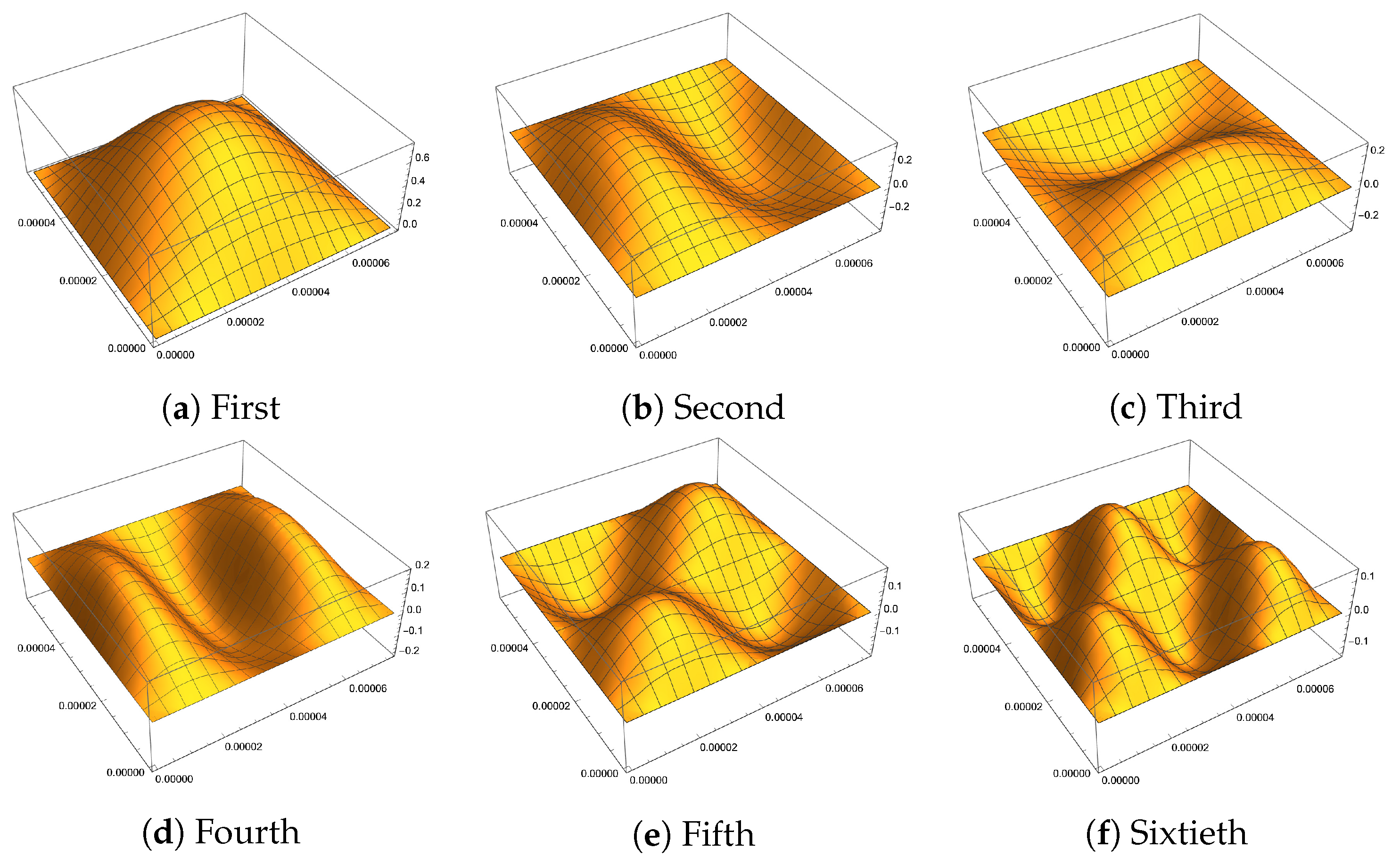
The eigenfunctions obtained by the FEM procedure with the $6\times 5$ mesh are indistinguishable from the exact ones. They are shown in Figure 1.

For specific geometries, for instance when the domain is rectangular, the boundary conditions are those as specified in the article and the material properties are constant, it is possible to obtain closed formulas for the eigenpairs. For other geometries and physical properties, in general, it is not possible. For the sake of generality, we chose to evaluate numerically the eigenvalues and use these computed values.

2.3.2. Validation for the Forced Motion

We start considering the same simply supported nanoplate of the previous section lying on the rectangle $\Omega =]0,L_X[\times ]0,L_Y[$ and driven by a dynamic load given by $g{\rho }_0\cos \left({\omega }_{0}t\right)S_1$, where $S_1$ is the first eigenfunction of the problem (12) and (13), with ${\omega }_0=8\times {10}^4$ rad/s. The solution u of the forced motion problem satisfies

$$\{\begin{array}{lll}{\rho }_0{u}_{,tt}+p_2{\Delta }^{2}u-p_1{\Delta }^{3}u=g{\rho }_0\cos \left({\omega }_{0}t\right)S_1,\hfill & \mathrm{in} ]0,\mathcal{T}[\times \Omega ,\hfill & \left(16\right)\\ \\ u=u_{,nn}=u_{,nnnn}=0,\hfill & \mathrm{on} ]0,\mathcal{T}[\times \partial \Omega ,\hfill & \left(17\right)\\ \\ u=u_{,t}=0,\hfill & \mathrm{at} \{t=0\}\times \Omega ,\hfill & \left(18\right)\\ \end{array}$$

where the number $g=9.8$ ms${}^{-2}$ stands for the acceleration of gravity.

By supposing $u(t,x,y)={\sum }_{k=1}^{+\infty }{g}_k\left(t\right)S_k(x,y)$, substituting in (16), using (12) and the orthogonality relations of the eigenfunctions, we obtain

$$u(t,x,y)=\frac{g{\rho }_0(\cos \left({\omega }_{0}t\right)-\cos \left({\lambda }_{1}t\right))}{{\lambda }_1^2-{\omega }_0^2}{S}_1(x,y),$$

(19)

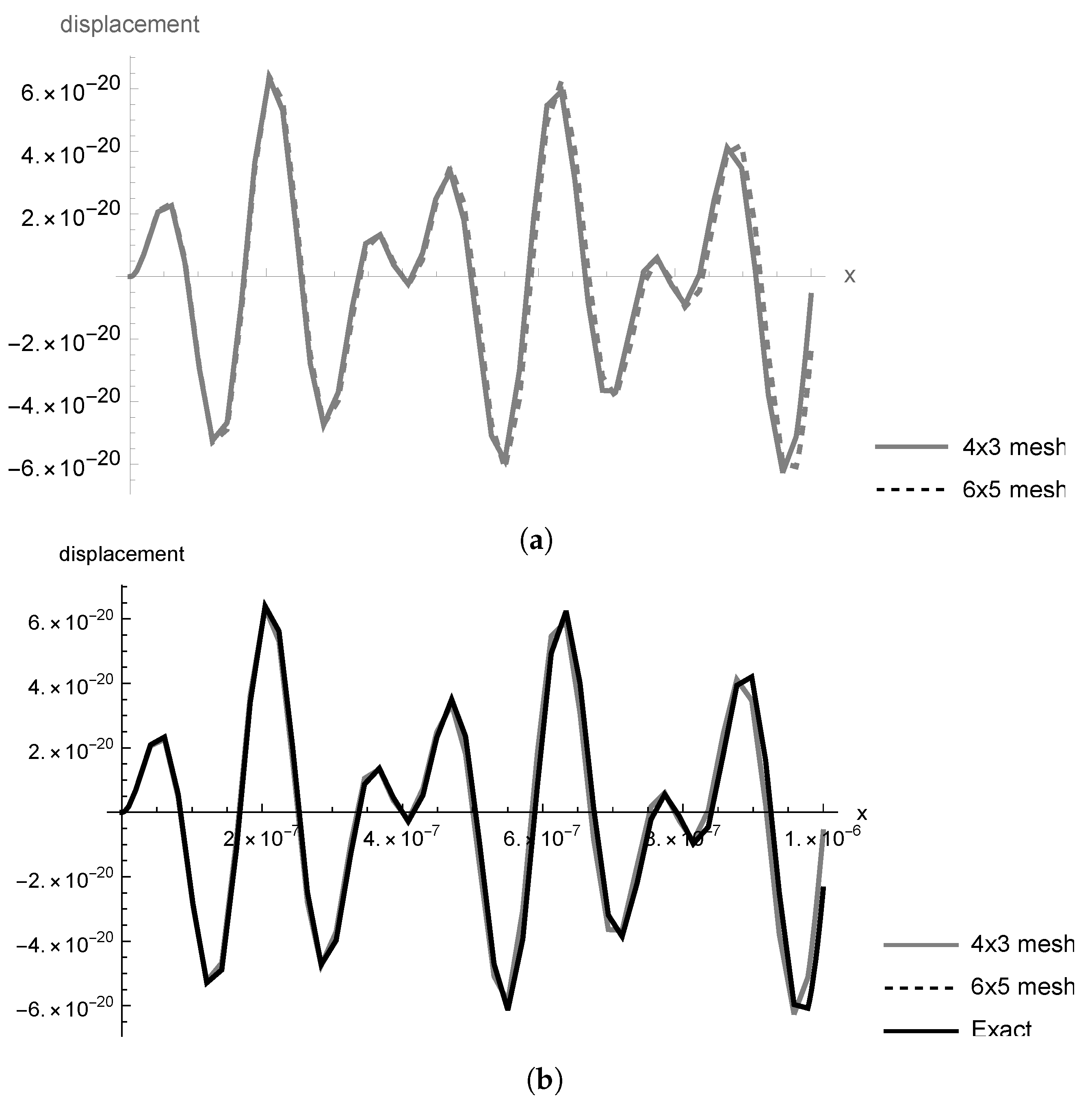
which is the exact solution of (16)–(18). We compare it with the solution obtained by the Finite Element Method with meshes of $6\times 5$ and $4\times 3$ elements. The results for the point $(\frac{L_X}{2},\frac{L_Y}{3})$ and time interval $[0,{10}^{-3}]$ s are shown in Figure 2. In Figure 2a we compare the results obtained with meshes with $6\times 5$ and $4\times 3$ elements. When we put them together with the graph of the exact solution (19) in Figure 2b, we see that it is indistinguishable from the result obtained by the Finite Element Method with a mesh of $6\times 5$ elements.

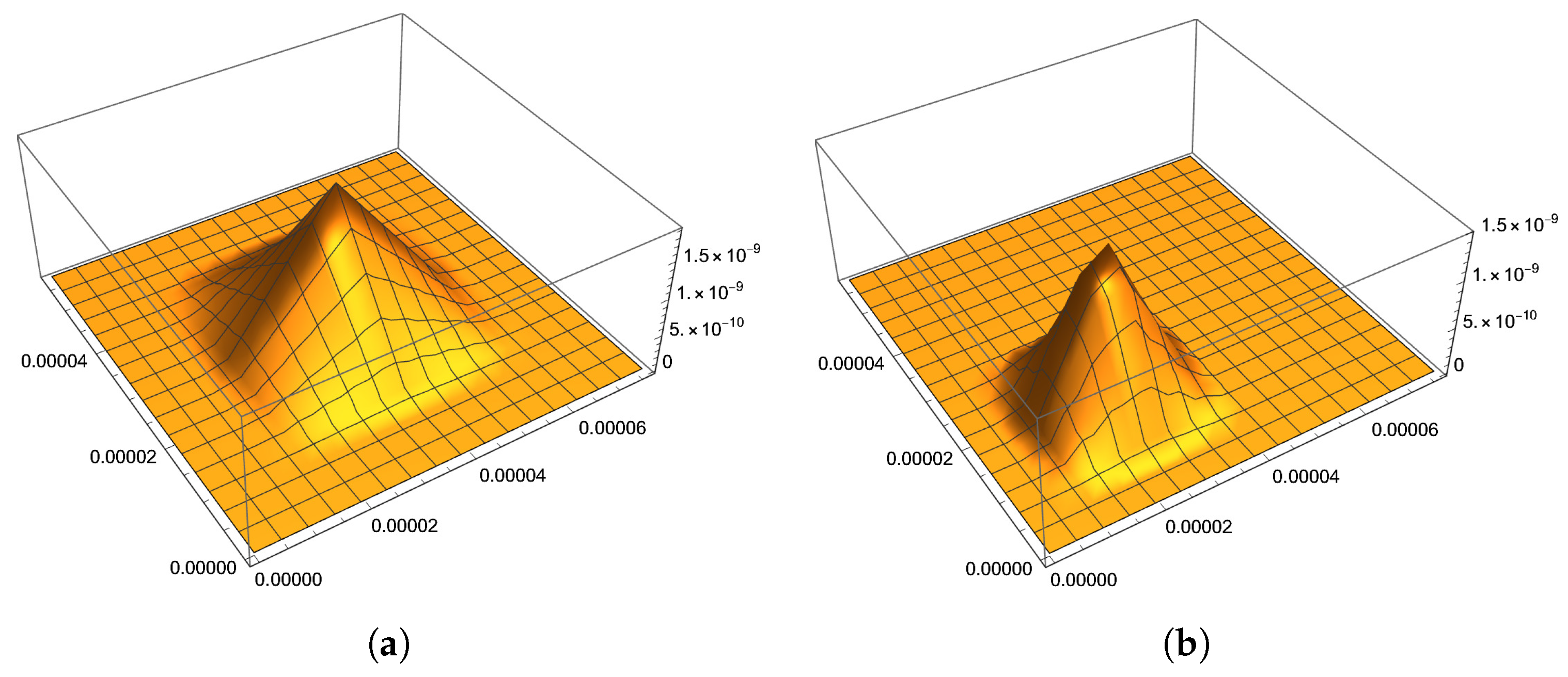
In anticipation of the inverse problem, next we consider the load $g_1\left(t\right)f_1\left(x\right)+g_2\left(t\right)f_2\left(x\right)$, where $g_j\left(t\right)=\cos \left({\omega }_{j}t\right)$, $j=1,2$, with ${\omega }_1=8\times {10}^4$ rad/s, ${\omega }_2=1\times {10}^5$ rad/s when the nanoplate starts from the rest. The spatial loads $f_1$ and $f_2$ are assumed of pyramidal shape as shown in Figure 3.

$f_1$ and $f_2$ taken to be

$$\begin{array}{cc}\hfill f_1(x,y)& =1.89\times {10}^{-9}\Lambda \left(\frac{x-L_1/2}{0.3L_1}\right)\Lambda \left(\frac{y-L_2/2}{0.3L_2}\right),\hfill \\ \hfill f_2(x,y)& =1.89\times {10}^{-9}\Lambda \left(\frac{x-L_1/3}{0.2L_1}\right)\Lambda \left(\frac{y-L_2/3}{0.2L_2}\right),\hfill \end{array}$$

(20)

where $\Lambda :\mathbb{R}\to \mathbb{R}$ is given by $\Lambda \left(x\right)=0$, if $\left|x\right|>1$ and $\Lambda \left(x\right)=1-\left|x\right|$, if $x\in [-1,1]$. The magnitude $1.89\times {10}^{-9}$ N/m² corresponds to ten times the weight per unit area of the specimen. The forces $f_1$ and $f_2$ are given in Pa.

Let us denote by $N_{df}$ and $N_f$ the number of degrees of freedom of the FE model and the number of terms used in the truncated series representation of the forcing terms, respectively.

By using the subset ${\left(S_n\right)}_{n=1}^{N_f}\subset {\left(S_n\right)}_{n=1}^{N_{df}}$ of the eigenbasis ${\left(S_n\right)}_{n=1}^{+\infty }$ we obtain the projection of the loads $f_1$ and $f_2$ into the space generated by ${\left(S_n\right)}_{n=1}^{N_f}$, that is, we obtain their numerical truncated Fourier representations:

$$f_j=\sum _{k=1}^{N_f}{\lambda }_k^2{\alpha }_{j,k}{S}_k,j=1,2.$$

(21)

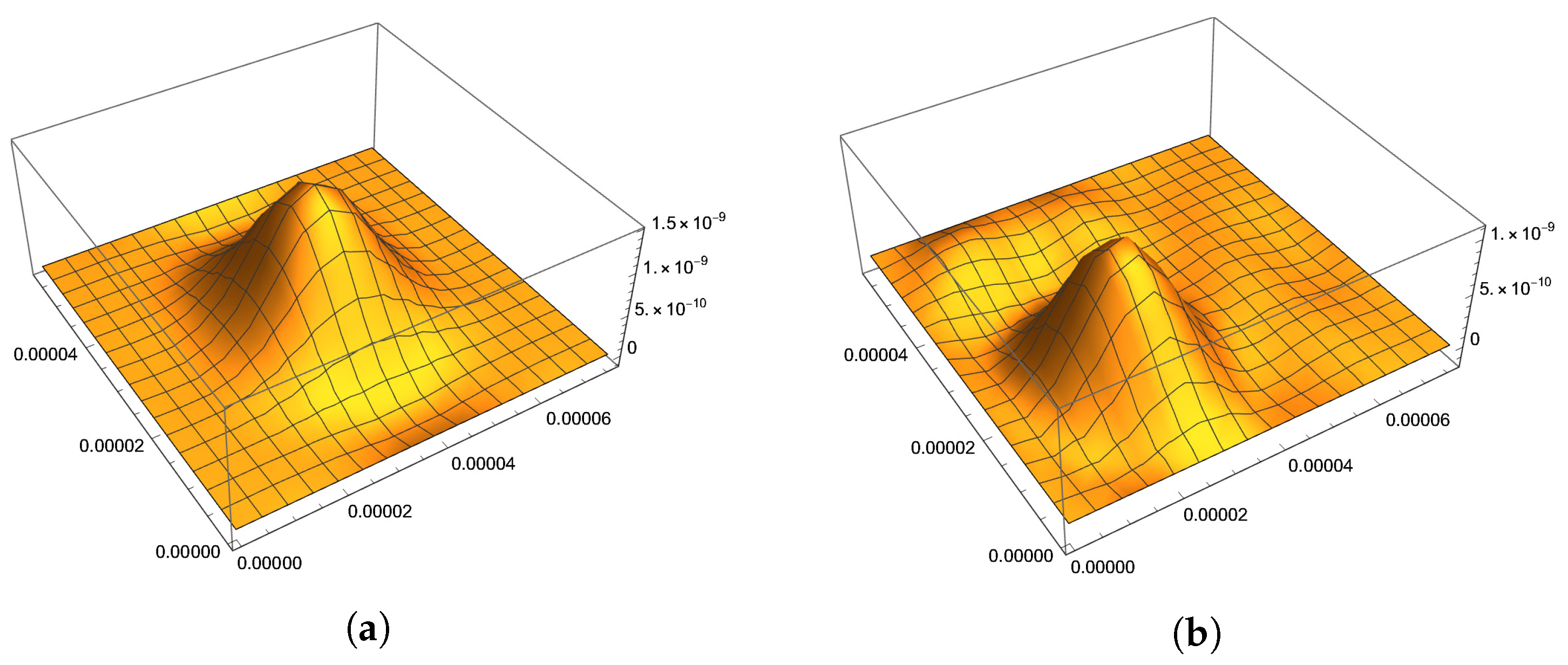
In the recovery algorithm, the loads $f_j$, $j=1,2$, are substituted by their truncated Fourier series representation, according to (21), which in turn become the target loads to be identified. In Figure 4 are shown the corresponding approximations of $f_1$ and $f_2$ with $N_f=40$.

The solution to the motion problem with the forced term $g_1\left(t\right)f_1\left(x\right)+g_2\left(t\right)f_2\left(x\right)$ as above is given by

$$u(t,x,y)=\sum _{j=1}^M\left\{\cos \left({\omega }_{j}t\right)\left[\sum _{k=1}^{+\infty }{A}_{j,k}{S}_k(x,y)\right]-\sum _{k=1}^{+\infty }\left[A_{j,k}{S}_k(x,y)\cos \left({\lambda }_{k}t\right)\right]\right\},$$

(22)

where $M=2$, which reflects the fact that we have just two asynchronous load components, and

$$A_{j,k}=\frac{{\alpha }_{j,k}{\lambda }_k^2}{{\lambda }_k^2-{\omega }_j^2},j=1,2,k\ge 1.$$

(23)

The truncated version of (22) determined by the first $N_{df}$ eigenfunctions only is obtained naturally.

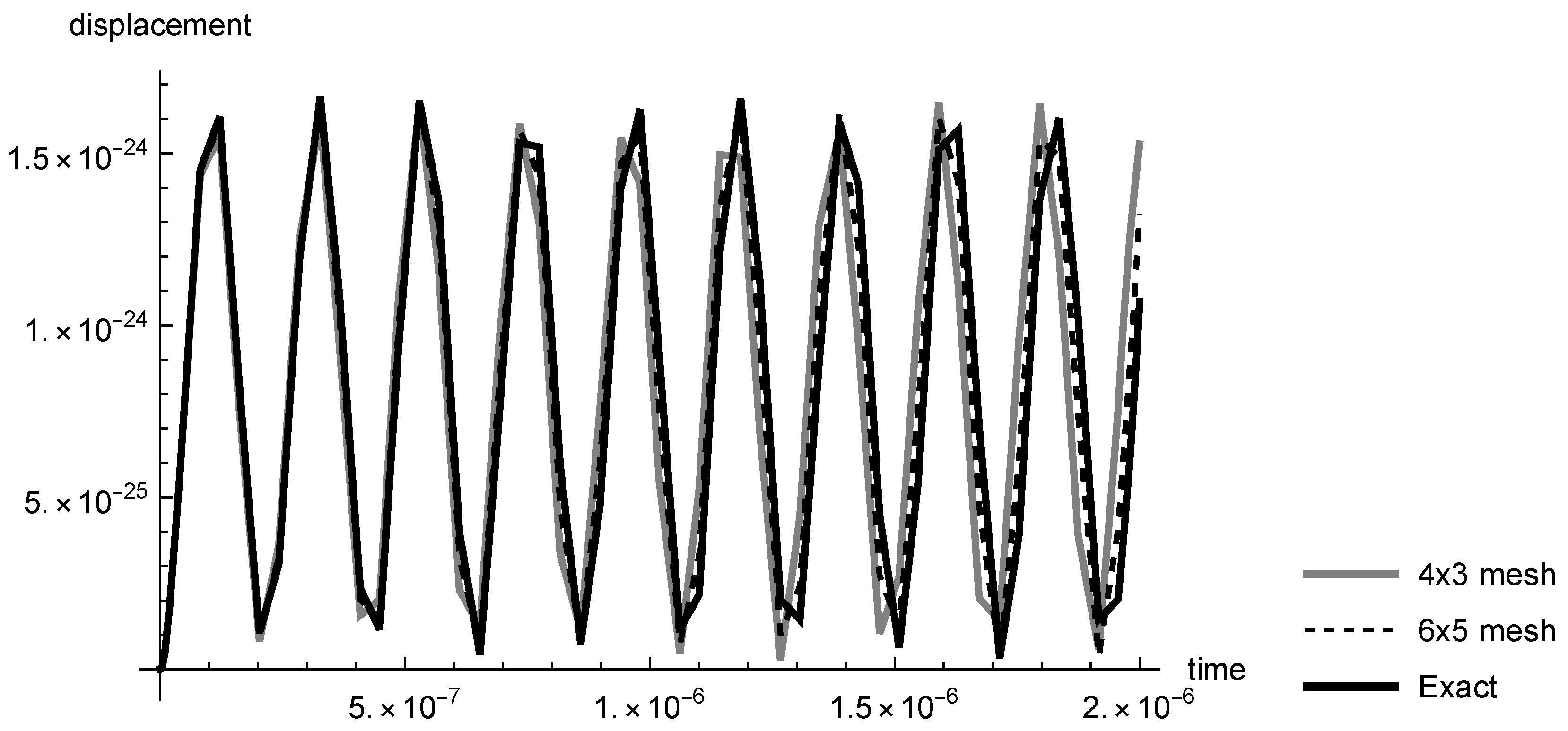
In Figure 5, we show the results for the displacement history at the point $(\frac{L_X}{2},\frac{L_Y}{3})$ in the time interval $[0,2\times {10}^{-6}]s$. The exact solution is evaluated via the spectral method by Formula (22).

The results indicate that the FE solution is very close to the exact solution of the motion problem (16)–(18) and, therefore, we decided to fix the $6\times 5$ mesh in performing the next simulations in Section 4. This choice provides a good compromise between the required accuracy and the computational burden.

In conclusion, we note that if we replace the eigenvalues and eigenfunctions corresponding to different boundary conditions in Equation (22), then the expression of u given by (22) would also represent the solution of the motion problem for the nanoplate under other boundary conditions.

3. A Uniqueness Result on Spatial Load Recovering and a Reconstruction Algorithm

Let us suppose that all the parameters in (4)–(6) are known, except for $f_m\in {\mathcal{P}}^{\prime }$, $m\in \{1,\dots ,M\}$, which are the unknown functions of the inverse problem. We start recalling a uniqueness result, proved in [1], on the determination of the spatial load components ${\left\{f_m\right\}}_{m=1}^M$ by measuring the transverse response of the nanoplate in a subset of $\Omega$ for an arbitrarily small interval of time.

In addition to the previous assumptions on the loads, here we suppose that $\{g_1,\dots ,g_M\}$ is a linearly independent set of functions on any interval $I\subset ]0,\mathcal{T}[$, namely if there is $I\subset ]0,\mathcal{T}[$ such that ${\sum }_{m=1}^M{c}_m{g}_m\left(t\right)=0$ for every $t\in I$, then $c_m=0$ for every $m=1,\dots ,M$.

The following uniqueness result was proved in [1].

Theorem 1. 

Let us denote by $u_{F_1}$, $u_{F_2}$ the solution to problem (4)–(6) corresponding to the set $F_1=\{f_1,\dots ,f_M\}$, $F_2=\{{\tilde{f}}_1,\dots ,{\tilde{f}}_M\}$, respectively. Under the above assumptions, if there is a nonempty open set $\tilde{\Omega }\subset \Omega$ and $T_0>0$ such that $u_{F_1}{{|}_{[0,T_0[\times \tilde{\Omega }}=u_{F_2}|}_{[0,T_0[\times \tilde{\Omega }}$, then $f_i={\tilde{f}}_i$ in Ω for $i=1,\dots ,M$.

We refer to reference [1] (Section 5) for a complete proof of Theorem 1. Here, we point out that the main mathematical tool on which the proof is based is different from that adopted by the authors in other contexts. In [20], for example, it was possible to take advantage of the fact that the set of eigenvalues of the problem constitutes a uniformly discrete sequence, i.e., there is a minimum separation quantity between an arbitrary pair of eigenvalues, and this allowed the application of specific properties of quasi-periodic distributions to prove uniqueness in the determination of the spatial component of the load. Adaptations of this idea were also developed by the authors to study the identification of a prey by the spider in an orb-web [21,22]. Unfortunately, the sequence of eigenvalues of the nanoplate, even for a rectangular domain, is not necessarily uniformly discrete, which is precisely why a proof based on spherical means was adopted to recover some unique continuation properties of the solution of the dynamic problem.

The methodology used in the proof of the above uniqueness result suggests a strategy for an approximate reconstruction of the spatial load. Referring to [1] for more details, in what follows we briefly describe the reconstruction algorithm that we shall use. Without loss of generality, we consider the nanoplate clamped at the boundary (see the motion problem (4)–(6) and the corresponding eigenvalue problem (8) and (9)).

We fix the observation time window $[0,T_0]$, $0<T_0<\mathcal{T}$, and a spatial observation set $\tilde{\Omega }\subset \Omega$ that, in practice, is taken to be the closure of a nonempty open set and may be nonconnected. Following [20], we introduce the family of functions

$${\varphi }_{m,\tau }\left(\xi \right)=\frac{\sin \left((\xi -{\lambda }_m)\tau \right)}{(\xi -{\lambda }_m)\tau },\forall m\in \mathbb{N},\forall \tau >0.$$

(24)

Observe that the Fourier transform of the functions ${\varphi }_{m,\tau }\left(\xi \right)$, which are going to be used as test functions in the time variable, is compactly supported, since

$$\widehat{{\varphi }_{m,\tau }}\left(t\right)=H_{\tau }\left(t\right){\mathrm{e}}^{-it{\lambda }_m},\forall m\in \mathbb{N},\tau >0,$$

(25)

where $H_{\tau }\left(t\right)=\frac{1}{2\tau }{\chi }_{]-\tau ,\tau [}$, $\forall \tau >0$, and ${\chi }_I$ is the characteristic function of the set I.

As test functions in the space variable, we use the functions

$${\phi }_j\left(x\right)=S_j\left(x\right){\chi }_{\tilde{\Omega }},\forall j\in \mathbb{N}.$$

(26)

The number of unknown loads is M. In this paper we limit the number of unknown forces to a maximum of 2, that is, we developed the analysis only for $M=1,2$. The extension to the case of more loads is straightforward.

Using u given by an expression analogous to (22) (written for clamped boundary conditions on $\partial \Omega$), we define

$$V_{0,\tau }\left(q\right)=\langle u,\widehat{{\varphi }_{q,\tau }}\otimes {\phi }_q\rangle ,V_{2,\tau }\left(q\right)=\langle \frac{{\partial }^{2}u}{\partial t^2},\widehat{{\varphi }_{q,\tau }}\otimes {\phi }_q\rangle ,q\in \{1,\dots ,N_{df}\},$$

(27)

observing that when we have just one load $f=f_1$, only $V_{0,\tau }\left(q\right)$ is used in the algorithm. Physically, $V_{0,\tau }$ corresponds to observing the displacement, whereas $V_{2,\tau }$ is related to the acceleration, which can be measured by accelerometers.

“We recall that $\widehat{\cos (\beta ·)}=\pi ({\delta }_{\beta }+{\delta }_{-\beta })$. It is simply the Fourier transform of the function $t\mapsto \cos \left(\beta t\right)$. It can be computed by recalling that $\cos \left(\beta t\right)=(e^{i\beta t}+e^{-i\beta t})/2$ and using the fact that the Fourier transform of $t\mapsto e^{i\beta t}$ is $\pi {\delta }_{\beta }$, where ${\delta }_{\beta }$ is the Dirac’s Delta distribution with support on the set $\left\{\beta \right\}$. The following next two formulas are simple consequences of (27) and the fact that $\widehat{\cos (\beta ·)}=\pi ({\delta }_{\beta }+{\delta }_{-\beta })$.”

$$\sum _{j=1}^M\sum _{k=1}^{N_{df}}\left\{\pi \langle S_k,{\phi }_q\rangle \left[{\Phi }_{q,\tau }\left({\omega }_j\right)-{\Phi }_{q,\tau }\left({\lambda }_k\right)\right]\right\}{A}_{j,k}=V_{0,\tau }\left(q\right),$$

(28)

and if $M=2$, we use also $V_{2,\tau }$. In this case,

$$\sum _{j=1}^M\sum _{k=1}^{N_{df}}\left\{\pi \langle S_k,{\phi }_q\rangle \left[-{\omega }_j^2{\Phi }_{q,\tau }\left({\omega }_j\right)+{\lambda }_k^2{\Phi }_{q,\tau }\left({\lambda }_k\right)\right]\right\}{A}_{j,k}=V_{2,\tau }\left(q\right),$$

(29)

where ${\Phi }_{q,\tau }\left(\xi \right)=({\varphi }_{q,\tau }\left(\xi \right)+{\varphi }_{q,\tau }(-\xi ))$ and $\langle S_k,{\phi }_q\rangle$ means just the integration of $S_k{\phi }_q$ over $\Omega$. From now on, we specialize the discussion to the case $M=2$.

In Equations (28) and (29), the variables $A_{j,k}$, $j=1,M=2$, encapsulate the unknowns ${\left({\alpha }_{j,k}\right)}_{k=1}^{N_{df}}$, $j=1,2$ (see Equation (23)), and the right hand sides $V_{0,\tau }\left(q\right)$ and $V_{2,\tau }\left(q\right)$ are obtained by measurement, which constitutes our data. Recall again that when there is only one load $f=f_1$, we use only the observation data $V_{0,\tau }\left(q\right)$.

Using (28) and (29), with $q=1,\dots ,N_{df}$, and $\tau =T_0$, we set up a matrix equation of the form

$$\left[\mathrm{TN}\right]\left[A\right]=\left[V\right],$$

(30)

where $\left[\mathrm{TN}\right]$ is a $\left(M{N}_{df}\right)\times \left(M{N}_{df}\right)$ square symmetric matrix. Furthermore, explicitly we have

$$\left[A\right]={[A_{1,1}{A}_{1,2}\dots A_{1,N_{df}}{A}_{2,1}{A}_{2,2}\dots A_{2,N_{df}}]}^t$$

(31)

and

$$\left[V\right]={[V_{0,\tau }\left(1\right)V_{0,\tau }\left(N_{df}\right)\dots V_{2,\tau }\left(1\right)V_{2,\tau }\left(N_{df}\right)]}^t.$$

(32)

The elements of the matrix $\left[\mathrm{TN}\right]$ are given by

$${(\mathrm{TN})}_{i,j}=\{\begin{array}{ll}\pi \langle S_j,{\phi }_i\rangle \left[{\Phi }_{i,\tau }\left({\omega }_1\right)-{\Phi }_{i,\tau }\left({\lambda }_j\right)\right],\hfill & i\le N_{df},j\le N_{df}\hfill \\ \pi \langle S_j,{\phi }_I\rangle \left[{\Phi }_{I,\tau }\left({\omega }_2\right)-{\Phi }_{I,\tau }\left({\lambda }_j\right)\right],\hfill & i>N_{df},j\le N_{df}\hfill \\ \pi \langle S_J,{\phi }_i\rangle \left[-{\omega }_1^2{\Phi }_{i,\tau }\left({\omega }_1\right)+{\lambda }_J^2{\Phi }_{i,\tau }\left({\lambda }_J\right)\right],\hfill & i\le N_{df},j>N_{df},\hfill \\ \pi \langle S_J,{\phi }_I\rangle \left[-{\omega }_2^2{\Phi }_{I,\tau }\left({\omega }_2\right)+{\lambda }_J^2{\Phi }_{I,\tau }\left({\lambda }_J\right)\right],\hfill & i>N_{df},j>N_{df},\hfill \end{array}$$

where $I=(1+mod(i,N_{df}))$ and $J=(1+mod(j,N_{df}))$. $mod(a,b)$ is the integer remainder of the Euclidean division of a by b.

The solution of (30) leads to the set ${\left({\tilde{\alpha }}_{j,k}\right)}_{k=1}^{N_{df}}$, $j=1$, M = 2, which is an approximation of the unknowns ${\left({\alpha }_{j,k}\right)}_{k=1}^{N_{df}}$, $j=1,\dots ,M$. By using ${\left({\tilde{\alpha }}_{j,k}\right)}_{k=1}^{N_{df}}$, $j=1,M=2$, and (21) we obtain an approximation to the functions $f_j$, $j=1,M=2$. In this way, we recover the spatial loads.

To measure the discrepancy between the recovered functions and their respective targets $f_j$, we use the absolute quadratic error function $\mathrm{Error}\left(f_j\right)$, evaluated as

$$\mathrm{Error}\left(f_j\right)=\sqrt{\sum _{k=1}^{N_{df}}{\lambda }_k^2{({\tilde{\alpha }}_{j,k}-{\alpha }_{j,k})}^2},j\in \{1,\dots ,M\}.$$

(33)

The relative error ${\mathrm{Error}}_R\left(f_j\right)$ is evaluated by the formula

$${\mathrm{Error}}_R\left(f_j\right)=\frac{\mathrm{Error}\left(f_j\right)}{\sqrt{{\sum }_{k=1}^{N_{df}}{\lambda }_k^2{\alpha }_{j,k}}}.$$

(34)

4. Applications

We illustrate applications of the reconstruction algorithm presented in the previous section for the determination of the spatial forces $f_1$ and $f_2$ in Equation (22) in a rectangular nanoplate $\Omega$. In all these simulations, the nanoplate is supposed to be clamped at the boundary. As already noted in Section 3, we consider the observation time interval $[0,T_0]$ and we measure the dynamic response of the nanoplate over a rectangle $\tilde{\Omega }\subset \Omega$ centered at $(x_c,y_c)\in \Omega$ and with sides $2a$ and $2b$.

In what follows, to avoid committing an inverse crime [23], the observation data will be perturbed by an error. The error is described by means of a normally distributed random variable $N(0,{ϵ}_e)$ with zero means so that $z(1+N(0,{ϵ}_e))$ is the value of the data z corrupted with the noise of level ${ϵ}_e>0$.

Error is introduced by multiplying each element of $\left[V\right]$, given by (32), by $(1+N(0,{ϵ}_e))$. At each time the random variable $N(0,{ϵ}_e)$ is invoked, a different random number is generated.

For the reconstruction algorithm, we will focus mainly on three parameters that are related to the size of the matrices involved and to the number of unknowns to be determined. The first parameter is the number of degrees of freedom $N_{df}$ of the FE model, which coincides with the number of available eigenpairs ${\left(({\lambda }_n^2,S_n)\right)}_{n=1}^{N_{df}}$. The second parameter is the number $N_f$, $N_f\le N_{df}$, of terms used in the truncated series representation of the forcing loads $f_1$, …, $f_M$ (see (21)). Finally, the third parameter is $N_{Trunc}$, $N_{Trunc}\le N_f$, which is going to be used to truncate the whole problem to achieve an SVD-based regularization scheme.

In the next subsections, the results of certain parametric simulations are presented and discussed. The first set of simulations is geared to verify the influence of the size of the observation set $\tilde{\Omega }$ and its position inside $\Omega$. The second set is aimed at evaluating the influence of the character of the spatial load, considering bimodal and discontinuous loads. In the remaining simulations, we analyze the influence of the presence of multiple asynchronous loads and the aspect ratio of the nanoplate.

4.1. Influence of the Size of $\tilde{\Omega }$ and Its Position Inside $\Omega$

In this section we consider our specimen loaded with $f=f_1$ (that is, $M=1$), where $f_1$ is defined in (20). The solution to the direct problem is obtained by the Finite Element Method with a mesh of $6\times 4$ elements. With this mesh, after the imposition of the boundary conditions, we are left with $N_{df}=120$.

The load is $\cos \left({\omega }_{0}t\right)f_1$, with ${\omega }_0=7.65\times {10}^7$ rad/s and ${\rho }_0=4.43865\times {10}^{-3}$ kg/m${}^2$. For the representation of $f_1$ by using (21), we use $N_f=40$ in this and subsequent sections. The observation time interval is kept constant equal to $[0,T_0]$, $T_0=1.0\times {10}^{-7}$ s. For comparison, we notice that the period of the forcing load is $2\pi /{\omega }_0=8.21\times {10}^{-8}$ s and that $2\pi /{\lambda }_1=2.921\times {10}^{-7}$. The error level in all simulations is ${ϵ}_e=0.02$.

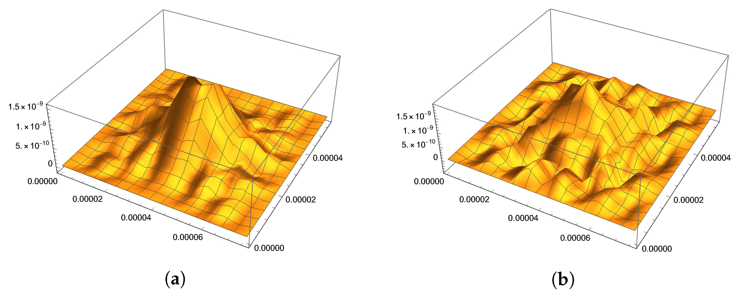
As expected, the smaller the observation set $\tilde{\Omega }\subset \Omega$, the worse the quality of the reconstruction. We compare the reconstruction results when $\tilde{\Omega }=]x_c-L_X/4,x_c+L_X/4[\times ]y_c-L_X/4,y_c+L_X/4[$ and $\tilde{\Omega }=]x_c-L_X/8,x_c+L_X/8[\times ]y_c-L_X/8,y_c+L_X/8[$, with $(x_c,y_c)=(L_X/2,L_Y/2)$. The results are shown in Figure 6, and in

Table 2. Absolute and relative errors. Influence of the size of the observation set.

$\tilde{\mathbf{\Omega }}$	$\mathbf{Error}\mathbf{\left(}{\mathit{f}}_{\mathbf{1}}\mathbf{\right)}$ (Pa)	${\mathbf{Error}}_{\mathit{R}}\mathbf{\left(}{\mathit{f}}_{\mathbf{1}}\mathbf{\right)}$
$]x_c-L_X/4,x_c+L_X/4[\times ]y_c-L_Y/4,y_c+L_Y/4[$	$6.24\times {10}^{-15}$	$0.25$
$]x_c-L_X/8,x_c+L_X/8[\times ]y_c-L_Y/8,y_c+L_Y/8[$	$1.349\times {10}^{-14}$	$0.53$

we show the absolute and relative errors in the reconstructions. For comparison, the target forcing term is shown in Figure 4a.

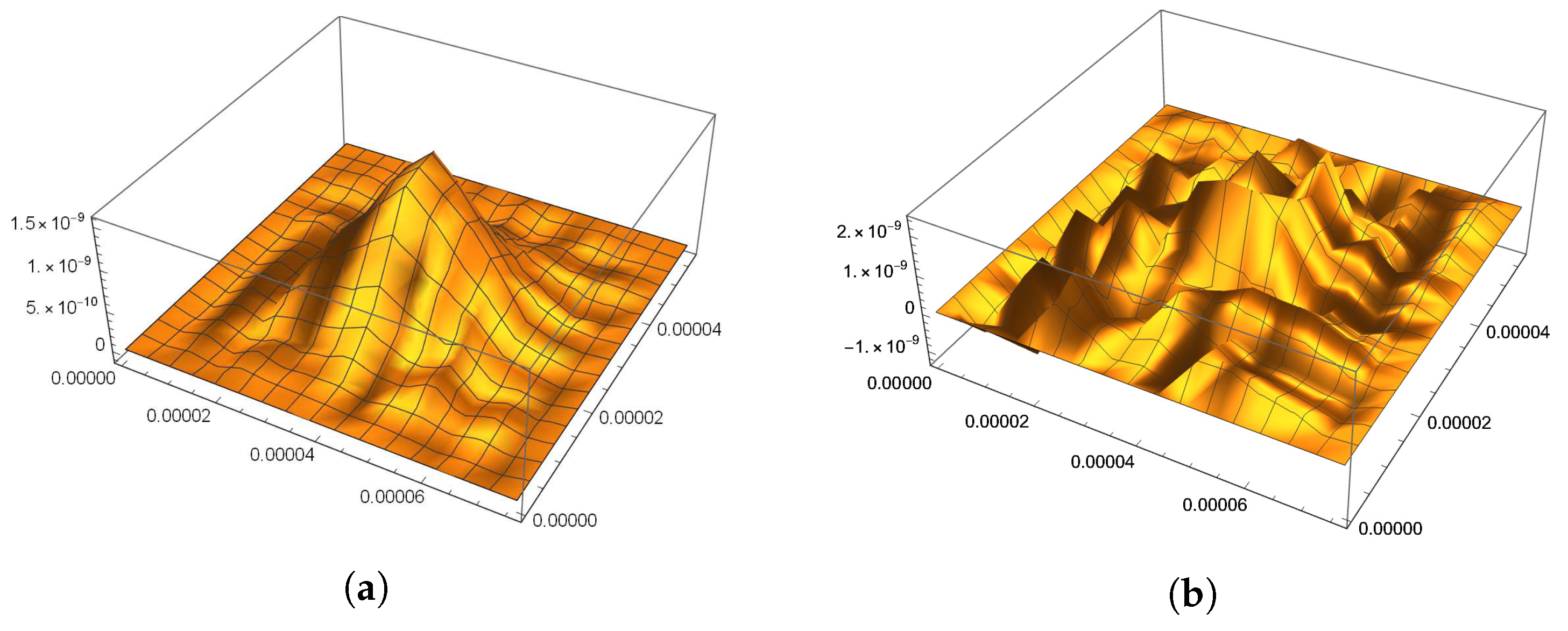
Keeping the same size of the observation set $\tilde{\Omega }=]x_c-L_X/4,x_c+L_X/4[\times ]y_c-L_X/4,y_c+L_X/4[$ used above, we move it away from the center. We show some results in Figure 7. The best reconstructions are obtained when $\tilde{\Omega }$ is closer to the center. The target load is still the one shown in Figure 4a.

The absolute and relative errors in the recovery process are shown in

Table 3. Absolute and relative errors. Influence of the position of the observation set.

Position of the Center	$\mathbf{Error}\mathbf{\left(}{\mathit{f}}_{\mathbf{1}}\mathbf{\right)}$ (Pa)	${\mathbf{Error}}_{\mathit{R}}\mathbf{\left(}{\mathit{f}}_{\mathbf{1}}\mathbf{\right)}$
$(x_c,y_c)=(L_X/3,L_Y/3)$	$4.55\times {10}^{-15}$	$0.18$
$(x_c,y_c)=(L_X/4,L_Y/4)$	$3.30\times {10}^{-14}$	$1.32$

.

4.2. Influence of the Character of the Spatial Load. Bimodal and Discontinuous Loads

All simulations of this section are developed with the observation set $\tilde{\Omega }=]x_c-L_X/4,x_c+L_X/4[\times ]y_c-L_X/4,y_c+L_X/4[$, $(x_c,y_c)=(L_X/2,L_Y/2)$, and using the observation time window $[0,T_0]$ with $T_0=1.0\times {10}^{-4}\mathrm{s}$.

We start by considering a bimodal spatial load. Specifically, the load, in S.I. units, that is, in Pa, to be recovered is given by

$$\begin{array}{cc}\hfill f(x,y)=1.89\times {10}^{-9}& \left[\Lambda \left(\frac{x-0.7L_1}{0.2L_1}\right)\Lambda \left(\frac{y-0.7L_2}{0.2L_2}\right)+\right.\hfill \\ \hfill & \left.+\Lambda \left(\frac{x-L_1/3}{0.2L_1}\right)\Lambda \left(\frac{y-L_2/3}{0.2L_2}\right)\right].\hfill \end{array}$$

(35)

The result shown in Figure 8 indicates that when there is only one force component, that is, $M=1$, the fact that whether the spatial load is unimodal does not influence the quality of the reconstruction. All parameters are the same as in the previous section, except for the error level that now is a bit higher, precisely ${ϵ}_e=0.05$. The absolute error of the reconstruction is $\mathrm{Error}\left(f_1\right)=1.40\times {10}^{-29}$, and the relative error is ${\mathrm{Error}}_R\left(f_1\right)=0.16$.

When we compare the quality of the reconstruction of continuous and discontinuous loads, we may infer that the regularity of the function that represents the load does influence the results in the expected way, in the sense that in reality what is being recovered is the truncated Fourier series that approximates the target function. The quality of the reconstruction is governed by the number of terms used in the truncated terms, and to well represent a less regular function, more terms are necessary, which leads to more numerical instabilities.

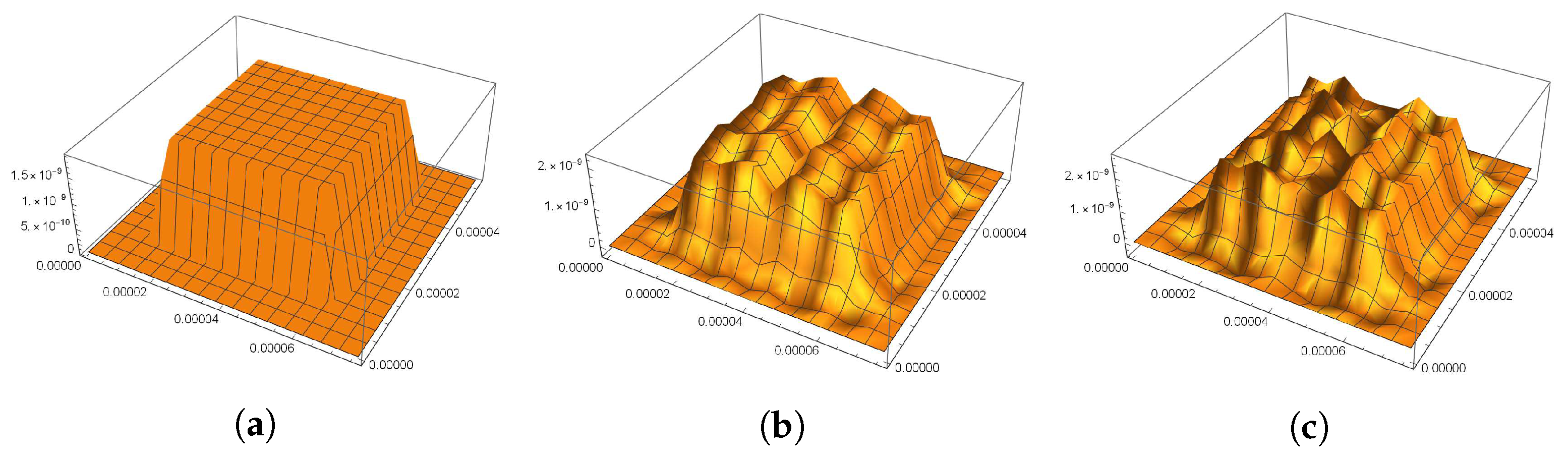
In Figure 9 we show the recovery result for the discontinuous load $f(x,y)=1.89\times {10}^{-9}{\chi }_A$, where $A=]L_X-L_X/3,L_X+L_X/3[\times ]L_Y-L_Y/3,L_Y+L_Y/3[$, with error level ${ϵ}_e=0.05$.

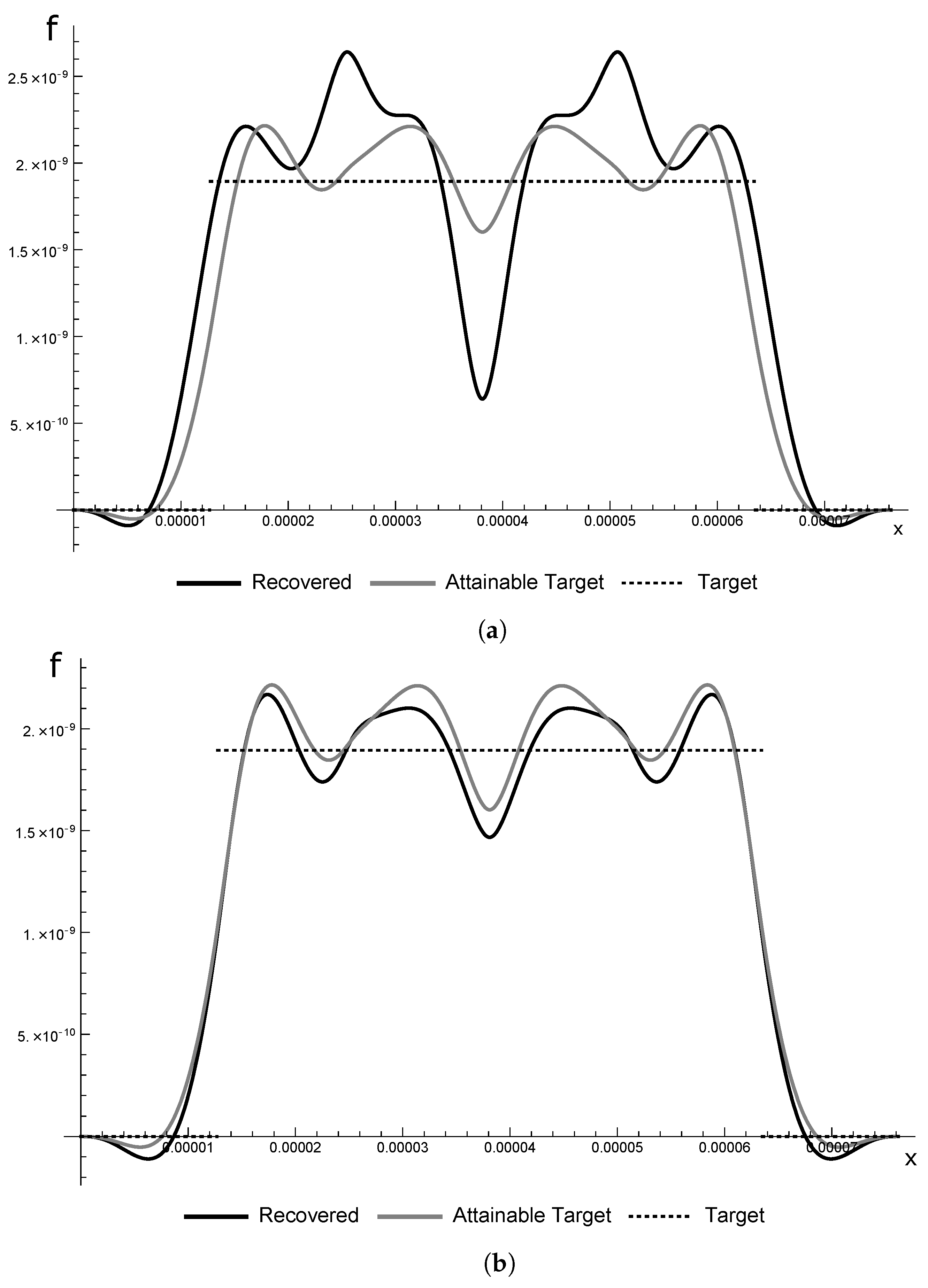
In Figure 10, we show the recovery results corresponding to two error levels, ${ϵ}_e=0.05$. and ${ϵ}_e=0.02$.

The corresponding absolute and relative errors in the recovery process are shown in

Table 4. Absolute and relative errors for the recovery of a discontinuous load.

Error Level	$\mathbf{Error}\mathbf{\left(}{\mathit{f}}_{\mathbf{1}}\mathbf{\right)}$ (Pa)	${\mathbf{Error}}_{\mathit{R}}\mathbf{\left(}{\mathit{f}}_{\mathbf{1}}\mathbf{\right)}$
${ϵ}_e=0.05$	$2.45\times {10}^{-14}$	$0.30$
${ϵ}_e=0.02$	$5.30\times {10}^{-15}$	$0.06$

.

Regularization Strategy

Up to this point, no special regularization strategies were employed, apart from natural discretization, which provides a certain degree of regularization. This was done to focus attention on the effects of the various parameters influencing the reconstruction. On the other hand, the quality of reconstruction can be poor without any regularization, as can be deduced from Figure 6b and Figure 7a,b. In the next section, we will see that when multiple asynchronous forces drive the dynamic system, the recovery process becomes more challenging, and, therefore, the use of some regularization strategy becomes a necessity.

Let us now explain the regularization strategy adopted in our simulations. It is based on the Singular Value Decomposition algorithm (see for instance [24,25]). In practice, we truncate the list of eigenvalues of the problem, keeping only the lowest ones, which is translated in the reduction of the order of the linear system (30). To implement the regularization, we use only the lowest $N_{Trunc}$ eigenvalues, where $N_{Trunc}=20$, assuming that all components of the unknown forces that correspond to eigenvalues greater than ${\lambda }_{N_{Trunc}}$ are null. To avoid committing an inverse crime [23], we hold the first $N_{Trunc}=20$ terms of the right-hand side of (30). When we apply this SVD-based strategy to get the recovered forces corresponding to Figure 7a,b, we obtain respectively the results shown in Figure 11a,b.

In the previous sections, where the implementation of this regularization strategy was not used, the linear system to be solved (30) involved $N_{df}$ unknowns for each $f_m$, $m=1,\dots ,M$, which can be interpreted also as a regularization by projection, but $N_{df}$ is relatively high. For instance, now in our simulations of this section, where $N_{Trunc}=20$, $N_{df}=120$.

The absolute and relative errors in the recovery process are shown in

Table 5. Absolute and relative errors for the recovery of a discontinuous load.

Error Level	$\mathbf{Error}\mathbf{\left(}{\mathit{f}}_{\mathbf{1}}\mathbf{\right)}$	${\mathbf{Error}}_{\mathit{R}}\mathbf{\left(}{\mathit{f}}_{\mathbf{1}}\mathbf{\right)}$
$(x_c,y_c)=(L_X/3,L_Y/3)$	$2.41\times {10}^{-30}$	$0.06$
$(x_c,y_c)=(L_X/4,L_Y/4)$	$1.63\times {10}^{-28}$	$0.51$

.

4.3. Multiple Asynchronous Loads

We show some results when the load driving the system is of the form $(g_1{f}_1+g_2{f}_2)$, with $f_j$, $j=1,2$, given in (20), and $g_j\left(t\right)=\cos \left({\omega }_{j}t\right)$, $j=1,2$. In this section, ${\omega }_1=7.65\times {10}^7$ rad/s, ${\omega }_2=2.48\times {10}^8$ rad/s. The corresponding direct problem was analyzed in Section 2.3.2.

This case, when two asynchronous loads are involved, is more challenging than when the loads are synchronous (cf. Section 4.2) for a specific reason that we explain now. Let us return to Equation (28) and note that, for each $q=1,\dots ,N_{df}$, it represents a line in the linear system of Equation (30), as can be noticed when we look at (31) and (32). We can split each line $q\in \{1,\dots ,2N_{df}\}$ of $\left[\mathrm{TN}\right]$ into two halves $[{\mathrm{TN}}_{q,1},\dots ,{\mathrm{TN}}_{q,N_{df}}]$ and $[{\mathrm{TN}}_{q,N_{df}+1},\dots ,{\mathrm{TN}}_{q,2N_{df}}]$. The first half is related to the unknowns ${\left\{A_{1,k}\right\}}_{k=1}^{N_{d}f}$, whereas the second half to ${\left\{A_{2,k}\right\}}_{k=1}^{N_{d}f}$. We see that the difference between the two halves $[{\mathrm{TN}}_{q,1},\dots ,{\mathrm{TN}}_{q,N_{df}}]$ and $[{\mathrm{TN}}_{q,N_{df}+1},\dots ,{\mathrm{TN}}_{q,2N_{df}}]$ is given by

$$[d_{q,1}{d}_{q,2}\dots d_{q,N_{df}}],$$

(21)

where

$$\{\begin{array}{ll}{d}_{q,k}\doteq \pi \langle S_k,{\phi }_q\rangle \left({\Phi }_{q,\tau }\left({\omega }_1\right)-{\Phi }_{q,\tau }\left({\omega }_2\right)\right)\hfill & \mathrm{if} q\le N_{df},\hfill \\ d_{q,k}\doteq \pi \langle S_k,{\phi }_q\rangle \left({\omega }_1^2{\Phi }_{q,\tau }\left({\omega }_1\right)-{\omega }_2^2{\Phi }_{q,\tau }\left({\omega }_2\right)\right)\hfill & \mathrm{if} q>N_{df}\hfill \end{array}$$

(37)

are very small numbers due to the nature of the functions involved, some numerical values being presented in the next simulations. As a consequence, from a numerical point of view, unless some special measures are not taken, the matrix $\left[\mathrm{TN}\right]$ will contain pairs of almost identical columns.

In other studies that we have been conducting in the past few years regarding the identification of loads [21,22], instead of using the function $\varphi$ given in (24), we used the square of it. The relevant mathematical property is that both versions possess compactly supported Fourier transforms. In physical terms, it amounts to say that the observation in time occurs in a bounded interval. The advantage of using ${\varphi }^2$ instead of $\varphi$ is that its Fourier transform is smoother but on the other hand, ${\varphi }^2$ decays faster, which means that the terms $d_{q,k}$ presented in (37) are even smaller. Therefore, the first of the special measures we took in this present work is to use $\varphi$ as in (24) and not the quadratic version as in our previous works.

The second special measure is to increase the internal precision of the calculations. We are using the software Mathematica, in which the standard precision, understood as the maximum number of extra digits to be used in functions, is 50. For the calculations that follow, we increased the precision to 200.

As in all simulations of this section, the observation set is $\tilde{\Omega }=]x_c-L_X/3,x_c+L_X/3[\times ]y_c-L_X/3,y_c+L_X/3[$, with $(x_c,y_c)=(L_X/2,L_Y/2)$ and the observation time window is $[0,T_0]$, $T_0=1.0\times {10}^{-7}\mathrm{s}$. The error level in all simulations is ${ϵ}_e=0.005$, and $N_{df}=40$.

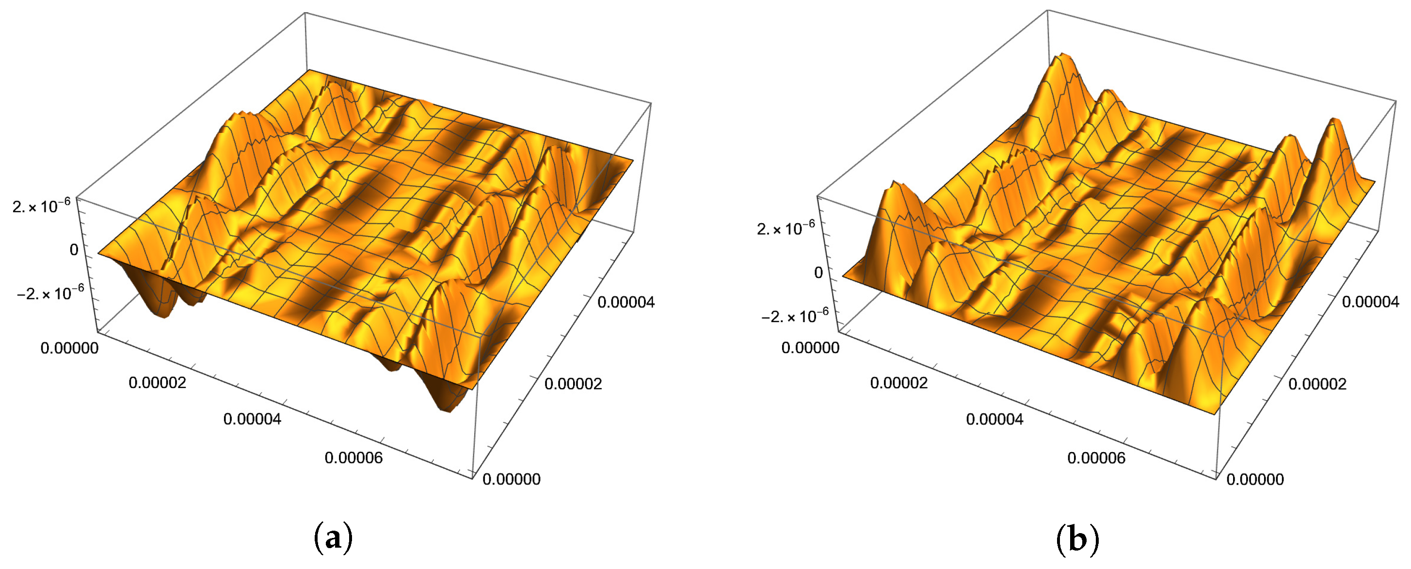
In Figure 12, we show the reconstruction results of the load $g_1{f}_1+g_2{f}_2$ described at the beginning of this section when there is no special regularization strategy apart from the natural discretization of the problem, which works as regularization method as explained in [25].

The de facto target loads shown in Figure 4 clearly could not be identified correctly.

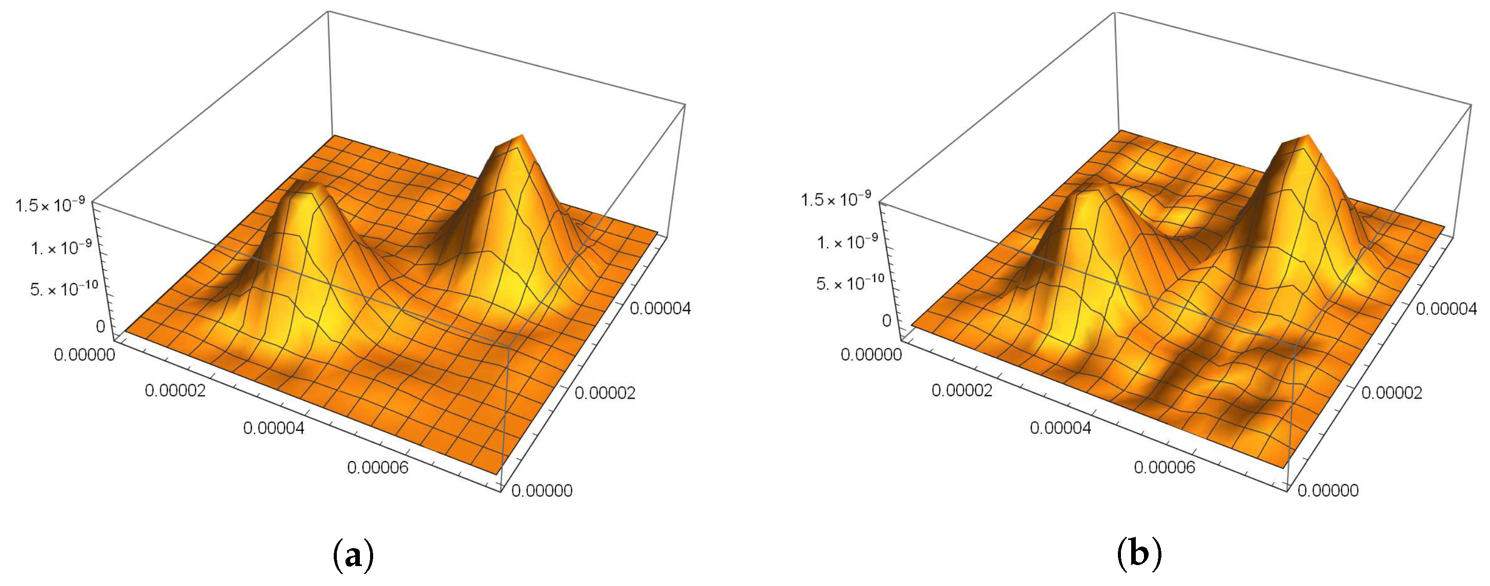
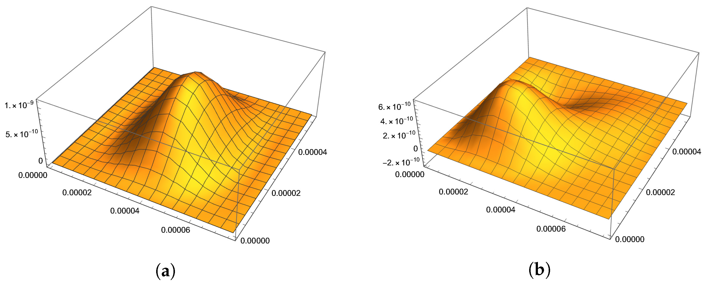
When we apply the SVD-based regularization strategy described above with $N_{Trunc}=12$, we obtain the results shown in Figure 13.

Although the recovered functions shown in Figure 13 are clearly not the same as the target ones shown in Figure 4, since, as expected, they are smoother than the targets, they correctly indicate the location and magnitudes.

Although we can say that the location of the peaks of both $f_1$ and $f_2$ and the order of their magnitudes were correctly estimated, the relative errors are high, as is shown in

Table 6. Absolute and relative errors. Influence of the application of the regularization strategy.

	${\mathit{L}}^{\mathbf{2}}$ Error		Relative ${\mathit{L}}^{\mathbf{2}}$ Error
	$\mathrm{Error}\left(f_1\right)$	$\mathrm{Error}\left(f_2\right)$	${\mathrm{Error}}_R\left(f_1\right)$	${\mathrm{Error}}_R\left(f_2\right)$
No SVD	$7.539\times {10}^{-22}$	$7.207\times {10}^{-22}$	$1099.0$	$1612.9$
$N_{Trunc}=12$	$4.011\times {10}^{-25}$	$9.546\times {10}^{-26}$	$25.25$	$18.56$

.

This can be explained by the fact that due to the instability of the problem, to get a meaningful answer we are forced to employ the SVD regularization strategy with a low value for $N_{Trunc}$. This means that $f_1$ and $f_2$ are estimated by using only the first few eigenfunctions, which are not enough to approximate them well. The results are smoother recovered functions, that approximate the targets, giving the information about their most salient properties, but nonetheless stay relatively far from them. The fact that absolute errors are very small means that even small deviations render the relative errors large.

We may infer from these results that the SVD-based strategy is a valuable instrument in our armory aimed at recovering unknown loads, but some more research is needed to explore new regularization schemes that improve the recovery process when two or more asynchronous loads are present.

4.4. Influence of Other Parameters

In this section, we perform additional simulations to explore the influence of other parameters in our inverse problem. Specifically, we investigate the influence of the aspect ratio of the rectangular domain $\Omega$, the thickness, and the mass density of the nanoplate on the quality of the recovery of the load.

4.4.1. Influence of the Thickness

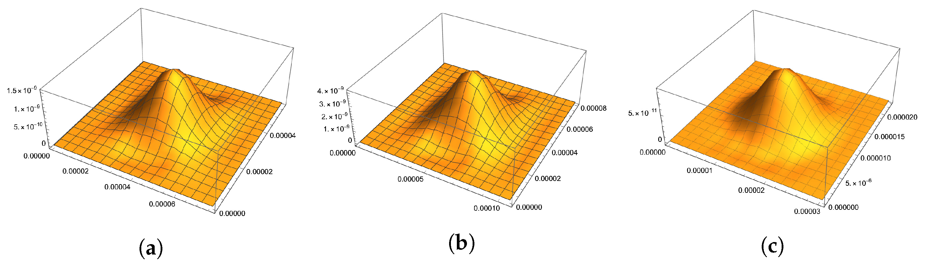
Applying our SVD-based regularization, we can verify the influence of the thickness on the quality of the result obtained when we run the identification algorithm. In Figure 14, we show the results corresponding to three thicknesses of the nanoplate. Except for the thickness, the parameters are the same as Section 4.1, with observation time interval $[0,T_0]$, $T_0=2.0\times {10}^{-8}\mathrm{s}$ and $N_{Trunc}=20$. The target function is shown in Figure 4a.

From several numerical experiments, the results seem to indicate that the thinner the nanoplate, the better the recovery results.

4.4.2. Influence of the Mass Density

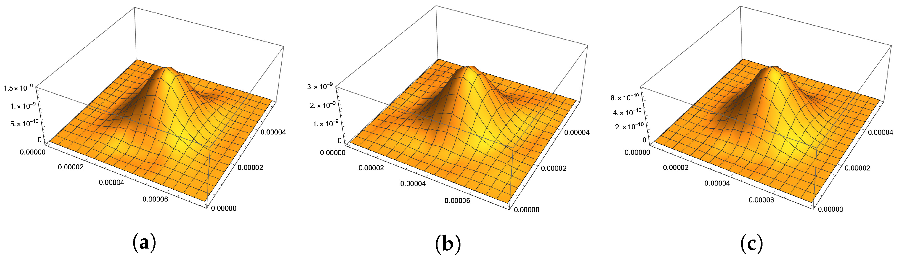
Some numerical experiments have been carried out by changing the mass density of the material. As in the last section, we apply our SVD-based regularization. Except for the mass density, the parameters are the same as Section 4.1, with thickness $h=$ 5 $l_0$, observation time interval $[0,T_0]$ for $T_0=2.0\times {10}^{-8}\mathrm{s}$, and $N_{Trunc}=20$. The target function is shown in Figure 4a.

The results of an extensive set of simulations seem to indicate that the less dense is the material of the nanoplate, the better are the recovery results. Figure 15 shows a representative set of results corresponding to three densities of the nanoplate.

4.4.3. Influence of the Aspect Ratio

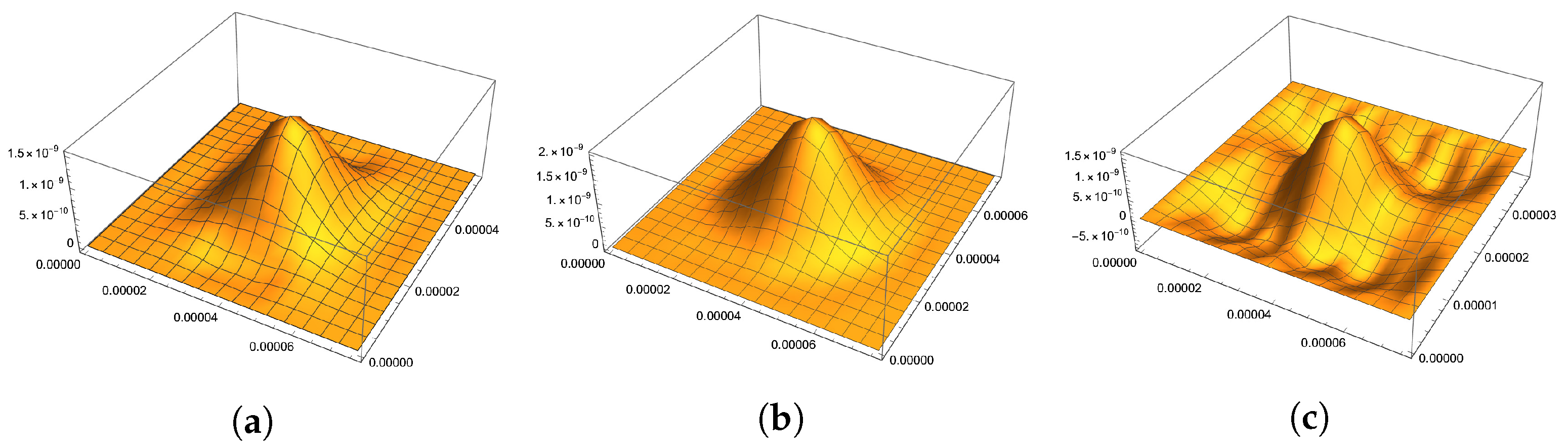
Finally, we consider the influence of the aspect ratio $\frac{L_X}{L_Y}$ on the spatial load reconstruction. We keep the same $6\times 5$ mesh used throughout the simulations, and to not severely distort the geometry of each element, we change slightly $L_Y$. Precisely, fixing $L_X$ we use in turn the values $L_Y=\frac{3L_X}{4},L_X,\frac{L_X}{2}$. We recall that the sides parallel to the $Ox$ axis of all elements are equal to $L_X/6$ and the sides of all elements have sides parallel to the $Oy$ axis equal to $L_Y/5$. The results are shown in Figure 16. It can be seen that the nanoplate with an aspect ratio near a square renders the best recovery results.

5. Conclusions

In this article, we developed a numerical implementation of a reconstruction technique of the transverse loads acting on a nanoplate. The observational data are the transverse displacement of the nanoplate in an open subset of its mid-plane, measured for an interval of time.

The reconstruction algorithm is based on the proof of the uniqueness result presented in [1], for the proof found therein suggests a constructive procedure. The loads treated here are of the form ${\sum }_{m=1}^M{g}_m\left(t\right)f_m(x,y)$, where $M\ge 1$, ${\left\{g_m\left(t\right)\right\}}_{m=1}^M$ is a known set of linear independent functions of the time variable, and the unknowns in this inverse problem are the functions ${\left\{f_m(x,y)\right\}}_{m=1}^M$.

A selected collection of numerical simulations for a nanoplate with a rectangular domain and the clamped boundary was presented and discussed. After validating the Finite Element algorithm for the direct problem, we analyzed the influence of several parameters on the recovery results, namely, the regularity of the spatial load distribution, the connectedness of the support of the spatial load distribution, the thickness of the nanoplate, the density of its material. Concerning the observation process, we analyzed the effect of the size of the observation set, in time and space, and also of its position inside the specimen. We also considered the influence of the number of asynchronous loads driving the system and the effect of a regularization strategy based on the SVD.

On the basis of our experience, we noticed that the use of a regularization strategy is essential, and the one that we used, based on the SVD concept, seems to work well. The factor that most influence the recovery results is the presence of asynchronous sources. When more than one is present, the identification of the individual spatial loads becomes extremely difficult. The reasons for this phenomenon were presented in Section 4.3. In our opinion, further research is needed to clarify this issue and to obtain an efficient and stable identification algorithm.

As for the other parameters, our results seem to follow what one should expect from physical grounds. The better the recovery results if the time interval is bigger, the observation spatial set is greater and centered around the center of the specimen. The fact that the load is more or less irregular in space or if it is composed of more than one connected component seems to be immaterial. On the other hand, the thickness, density of the material, and aspect ratio of the nanoplate definitely have an influence. The lighter the material, the thinner the specimen, and the closer the aspect ratio is to one, the better the identification results.

These findings may be useful as guidelines for the design of nanosensors aimed at the identification of unknown loads.

Finally, as is well known, the availability of stability estimates for our inverse problem can be useful to prove the convergence of regularised inversion procedures and also to quantify the rate of convergence; see, for example, [26]. This important issue has not been investigated in the present research and will be the subject of future studies.

References

- Kawano, A.; Morassi, A.; Zaera, R. Inverse load identification in vibrating nanoplates. Math. Methods Appl. Sci. 2023, 46, 1045–1075. [Google Scholar] [CrossRef]
- Lam, D.C.C.; Yang, F.; Chong, A.C.M.; Wang, J.; Tong, P. Experiments and theory in strain gradient elasticity. J. Mech. Phys. Solids 2003, 51, 1477–1508. [Google Scholar] [CrossRef]
- Thai, H.T.; Vo, T.P.; Nguyen, T.K.; Kim, S.E. A review of continuum mechanics models for size-dependent analysis of beams and plates. Compos. Struct. 2017, 177, 196–219. [Google Scholar] [CrossRef]
- Helbling, T.; Roman, C.; Durrer, L.; Stampfer, C.; Hierold, C. Gauge factor tuning, long-term stability, and miniaturization of nanoelectromechanical carbon-nanotube sensors. IEEE Trans. Electron Devices 2011, 58, 4053–4060. [Google Scholar] [CrossRef]
- Hurst, A.M.; Lee, S.; Petrone, N.; Weert, J.V.D.; Zande, A.M.V.D.; Hone, J. A transconductive graphene pressure sensor. In Proceedings of the 2013 Transducers & Eurosensors XXVII: The 17th International Conference on Solid-State Sensors, Actuators and Microsystems (2013), Barcelona, Spain, 16–20 June 2013; pp. 586–589. [Google Scholar]
- Khanna, V.K. Frontiers of nanosensor technology. Sens. Transducers 2009, 103, 1. [Google Scholar]
- Laukhin, V.; Sánchez, I.; Moya, A.; Laukhina, E.; Martin, R.; Ussa, F.; Rovira, C.; Guimera, A.; Villa, R.; Aguiló, J.; et al. Non-invasive intraocular pressure monitoring with a contact lens engineered with a nanostructured polymeric sensing film. Sens. Actuators A Phys. 2011, 170, 36–43. [Google Scholar] [CrossRef]
- Cheng, J.; Ding, G.; Yamamoto, M. Uniqueness along a line for an inverse wave source problem. Commun. Partial. Differ. Equ. 2002, 27, 2055–2069. [Google Scholar] [CrossRef]
- Hu, G.; Kian, Y.; Zhao, Y. Uniqueness to some inverse source problems for the wave equation in unbounded domains. Acta Math. Appl. Sin. 2020, 36, 134–150. [Google Scholar] [CrossRef]
- Alves, C.; Silvestre, A.L.; Takahashi, T.; Tucsnak, M. Solving inverse source problems using observability. Applications to the Euler-Bernoulli plate equation. SIAM J. Control. Optim. 2009, 48, 1632–1659. [Google Scholar] [CrossRef]
- Dempsey, K.M.; Grossman, N.; Vasileva, I.V. Force inversion in floating plate dynamics. Inverse Probl. 2006, 22, 381–397. [Google Scholar] [CrossRef]
- Arat, Z.; Khanmamedov, A.; Simsek, S. A unique continuation result for the plate equation and an application. Math. Methods Appl. Sci. 2016, 39, 744–761. [Google Scholar] [CrossRef]
- Yamamoto, M. Determination of forces in vibrations of beams and plates by pointwise and line observations. J. Inverse Ill-Posed Probl. 1996, 4, 437–457. [Google Scholar] [CrossRef]
- Kawano, A. Uniqueness in the determination of vibration sources in rectangular Germain–Lagrange plates using displacement measurements over line segments with arbitrary small length. Inverse Probl. 2013, 29, 085002. [Google Scholar] [CrossRef]
- Kim, J.U. Exact semi-internal control of an Euler-Bernoulli equation. SIAM J. Control. Optim. 1992, 30, 1001–1023. [Google Scholar] [CrossRef]
- Mindlin, R.D.; Eshel, N.N. On first strain-gradient theories in linear elasticity. Int. J. Solids Struct. 1968, 4, 109–124. [Google Scholar] [CrossRef]
- Munch, I.; Neff, P.; Madeo, A.; Ghiba, I.D. The modified indeterminate couple stress model: Why Yang et al.’s arguments motivating a symmetric couple stress tensor contain a gap and why the couple stress tensor may be chosen symmetric nevertheless. ZAMM J. Appl. Math. Mech. Z. Angew. Math. Mech. 2017, 97, 1524–1554. [Google Scholar] [CrossRef]
- Burnett, D.S. Finite Element Analysis; Addison-Wesley Publishing Company: Lebanon, IN, USA, 1987. [Google Scholar]
- Rahaeifard, M.; Ahmadian, M.T. On pull-in instabilities of microcantilevers. Int. J. Eng. Sci. 2015, 87, 23–31. [Google Scholar] [CrossRef]
- Kawano, A.; Zine, A. Uniqueness and nonuniqueness results for a certain class of almost periodic distributions. SIAM J. Math. Anal. 2011, 43, 135–152. [Google Scholar] [CrossRef]
- Kawano, A.; Morassi, A. Detecting a prey in a spider orb web. SIAM J. Appl. Math. 2019, 79, 2506–2529. [Google Scholar] [CrossRef]
- Kawano, A.; Morassi, A.; Zaera, R. Detecting a prey in a spider orb-web from in-plane vibration. SIAM J. Appl. Math. 2021, 81, 2297–2322. [Google Scholar] [CrossRef]
- Kaipio, J.; Somersalo, E. Statistical and Computational Inverse Problems; Applied Mathematical Sciences; Springer: Berlin/Heidelberg, Germany, 2004; Volume 160. [Google Scholar]
- Baumeister, J. Stable Solution of Inverse Problems; Vieweg, F., Braunschweig, S., Eds.; Springer: Berlin/Heidelberg, Germany, 1987. [Google Scholar]
- Kirsch, A. An Introduction to the Mathematical Theory of Inverse Problems, 3rd ed.; Springer: Berlin/Heidelberg, Germany, 2021. [Google Scholar]
- de Hoop, M.; Qiu, L.; Scherzer, O. Local analysis of inverse problems: Hölder stability and iterative reconstruction. Inverse Probl. 2012, 28, 045001. [Google Scholar] [CrossRef]
Figure 1.
First six eigenfunctions obtained by the FEM with a mesh.
Figure 2.
Comparison of the numerical time histories of the displacement function at the point . (a) Comparison between the results for and meshes. (b) Comparison between the results for and meshes with the exact solution.
Figure 3.
Spatial loads. (a) Load . (b) Load .
Figure 4.
Target loads. (a) Load . (b) Load .
Figure 5.
Comparison between the exact solution (solid line) and the approximate solution obtained by the FEM. Displacement history at the point .
Figure 6.
Comparison of the reconstruction results when we vary the size of the observation set . (a) . (b) .
Figure 7.
Comparison of the reconstruction results when we vary the position of the observation set . (a) . (b) .
Figure 8.
Comparison of the results when we vary the position of the observation set . (a) Attainable target load with two peaks. (b) Recovered load.
Figure 9.
Recovery of a discontinuous load. (a) Target load. (b) Attainable target load. (c) Recovered load (error level ).
Figure 10.
Recovery of a discontinuous load. (a) Sections of the recovered load on the line . Error level . (b) Sections of the recovered load on the line . Error level .
Figure 11.
Application of the SVD-based regularization strategy. (a) Recovery of the load corresponding to Figure 7a when the regularization strategy is applied with . (b) Recovery of the load corresponding to Figure 7b when the regularization strategy is applied with .
Figure 12.
Recovery of loads when there is no regularization. (a) Recovery of when there is no regularization. (b) Recovery of when there is no regularization.
Figure 13.
Recovery of loads when the SVD-based regularization is applied, with . (a) Recovery of with SVD-based regularization. . (b) Recovery of with SVD-based regularization. .
Figure 14.
Influence of the thickness. (a) Recovered load. Plate thickness = 5 . Relative error . (b) Recovered load. Plate thickness 7 . Relative error . (c) Recovered load. Plate thickness 2 . Relative error .
Figure 15.
Influence of the density. (a) Recovered load. Mass per unit area . Relative error . (b) Recovered load. Mass per unit area 0.2 . Relative error . (c) Recovered load. Mass per unit area 0.5 . Relative error .
Figure 16.
Influence of the aspect ratio. (a) Recovered load. Aspect ratio . Relative error . (b) Recovered load. Aspect ratio . Relative error . (c) Recovered load. Aspect ratio . Relative error .