
Theoretical Validation of New Two-Dimensional One-Variable-Power Copulas

Department of Mathematics, LMNO, Université de Caen-Normandie, 14032 Caen, France
Axioms 2023, 12(4), 392; https://doi.org/10.3390/axioms12040392
Submission received: 6 March 2023
/
Revised: 12 April 2023
/
Accepted: 14 April 2023
/
Published: 18 April 2023
(This article belongs to the Special Issue Statistical Modeling of Modern Multivariate Data)
Abstract
:One of the most effective ways to illustrate the relationship between two quantitative variables is to describe the corresponding two-dimensional copula. This approach is acknowledged as practical, nonredundant, and computationally manageable in the context of data analysis. Modern data, however, contain a wide variety of dependent structures, and the copulas now in use may not provide the best model for all of them. As a result, researchers seek to innovate by building novel copulas with appealing properties that are also based on original methodologies. The foundations are theoretical; for a copula to be validated, it must meet specific requirements, which frequently dictate the constraints that must be placed on the relevant parameters. In this article, we make a contribution to the understudied field of one-variable-power copulas. We first identify the specific assumptions that, in theory, validate copulas of such nature. Some other general copulas and inequalities are discussed. Our general results are illustrated with numerous examples depending on two or three parameters. We also prove that strong connections exist between our assumptions and well-established distributions. To highlight the importance of our findings, we emphasize a particular two-parameter, one-variable-power copula that unifies the definition of some other copulas. We reveal its versatile shapes, related functions, various symmetry, Archimedean nature, geometric invariance, copula ordering, quadrant dependence, tail dependence, correlations, and distribution generation. Numerical tables and graphics are produced to support some of these properties. The estimation of the parameters based on data is discussed. As a complementary contribution, two new, intriguing one-variable-power copulas beyond the considered general form are finally presented and studied.
Keywords:
one-variable-power copulas; dependence models; multidimensional analysis; correlation measuresMSC:
60E15; 62H991. Introduction
It is ideal to assume two-dimensional normality when trying to explain the dependence of two quantitative variables. In this case, the theory has been around for a while, and well-mastered practical tools exist. However, a straightforward data analysis can typically disprove the non-normality assumption. Furthermore, the relationship between the two variables can have a complex structure beyond the standard schemes. The copula method suggests a workable resolution. Before going further, let us briefly define what a copula is from a mathematical viewpoint. A cumulative distribution function (CDF) on whose unidimensional margin distributions are uniformly distributed is known as a two-dimensional copula. The well-known Sklar’s theorem has helped copulas gain a lot of attention (see [1,2]). It asserts that every two-dimensional CDF can be expressed using the proper copula and its marginal CDFs. In this sense, a copula can be viewed as a dependence-related function. It is also a helpful tool for creating two-dimensional distributions. We refer to [3,4,5] for a complete view of the copula theory and a few of its uses. In the last few decades, numerous techniques have been developed for creating new copulas as a result of the increasing significance of dependence analysis in various statistical scenarios. The aim is to produce more adaptable families of two-dimensional CDFs that have a variety of attractive characteristics, such as tail dependence properties, asymmetries, broad correlation ranges, and probability density functions with original and flexible shapes. On these aspects, recent developments can be found in [6,7,8,9,10,11,12,13,14,15,16,17]. More specifically, in [11], some modifications of the Farlie–Gumbel–Morgenstern copula are proposed; in [13], a family of positive quadrant-dependent two-dimensional copulas is elaborated; in [17], Baker–Lin–Huang-type two-dimensional copulas based on order statistics are developed; in [9], some copulas are constructed from the pairs of order statistics; in [14], a family of two-dimensional independent copula transformations is studied; in [12], new types of multidimensional trigonometric copulas are proposed; in [15], various original three- and two-dimensional ratio-power copulas are developed; in [6], a collection of new trigonometric and hyperbolic Farlie–Gumbel–Morgenstern-type copulas are established; in [7], two generalized two-dimensional Farlie–Gumbel–Morgenstern copulas and rank reduction are investigated; in [10], two-dimensional copulas based on the counter-monotonic shock method are given; in [16], a multidimensional extension of the Raftery copula is proposed; and in [8], an extension of the Gumbel–Barnett family of copulas is studied.
In particular, in [8,18], copulas of the following form are studied:
where is a tuning parameter and and are differentiable continuous functions. Of course, the admissible values for are directly connected to the definitions of and . The form in Equation (1) is general. In particular, it includes the Gumbel–Barnett copula, obtained with and (see [5]), and the Celebioglu–Cuadras copula, which appears by taking and (see [19,20,21]). Furthermore, in the very special case where , and and , we obtain
which has been proposed in ([18] Example 2.3) (see also ([8] Exemple 3)). This specific one-variable-power (OVP) copula form is inspirational; to the best of our knowledge, there is no in-depth study on copulas expressed as
where denotes a function that is only dependent on x (not y). Some motivations for considering it are listed below. This form is less general (and more simple) than the one in Equation (1), and it allows us to reveal some admissible functions with a high level of originality or complexity. In particular, as sketched in Equation (2), two- or three-parameter special functions for are quite conceivable. This is not the case when dealing with two functions that are dependent on different variables, such as and .
We thus open this new room of research with the following contributions:
- (i)
- We determine the precise assumptions on that allow the two-dimensional function in Equation (2) to be a valid copula.
- (ii)
- By using the flipping and survival methods, we derive some new general copulas with similar OVP functionalities.
- (iii)
- Based on our copula findings, we derive some new general OVP two-dimensional inequalities.
- (iv)
- We illustrate our general results with some concrete functions depending on two or three tuning parameters and exhibit some connections between the assumptions made on and well-established truncated lifetime distributions.
- (v)
- We thoroughly investigate a particular proposed copula, emphasizing its related functions, shapes, various symmetry, Archimedean nature, geometric invariance, copula ordering, quadrant dependence, tail dependence, correlations, and distribution generation.
- (vi)
- A short statistical work is given to illustrate how the involved parameters of this particular copula can be estimated from data.
- (vii)
- Two new OVP copulas beyond the form in Equation (2) are finally presented as an additional contribution; one of them can be viewed as an original modified OVP version of the so-called Ali–Mikhail–Haq copula.
Typically, the proposed copulas may be used to model various claim types, payment and incurred loss data, and cross-industry- and cross-breach-type structures for monthly cyber losses, as well as the mortality of some countries, in the spirit of [22,23,24] with existing exponential–logarithmic-type copulas.
The rest of the article is organized as follows: Our general results are given in Section 2, along with some examples. Section 3 is devoted to the in-depth study of the suggested copula. Section 4 provides additional contributions by validating intriguing OVP copulas. The conclusion is given in Section 5.
2. OVP Variable Copulas
2.1. General Results
To begin, let us recall the exact mathematical definition of an absolutely continuous two-dimensional copula.
Definition 1
(absolutely continuous two-dimensional copulas [5]). A two-dimensional function , is said to be an absolutely continuous two-dimensional copula if and only if the following assumptions are met for any :
- (I)
- and ;
- (II)
- and ;
- (III)
- , where represents the standard (mixed-second-order) partial derivatives according to x and y.
This definition is at the heart of most of our proofs. In the rest of the paper, we omit the sentence “absolutely continuous two-dimensional” to lighten the text.
The following result presents the general assumptions made on to make copulas of the form valid.
Theorem 1.
Let , be a function satisfying the following assumptions:
- A1:
- (or );
- A2:
- with ;
- A3:
- differentiable for with (so that is non-increasing);
- A4:
- .
Then, the following two-dimensional OVP function is a copula:
with the usual convention that exists, i.e., equal to a finite value.
Proof.
The proof consists in demonstrating that satisfies the points (I), (II) and (III) of Definition 1.
- Proof
- for (I) To begin, let us consider . For any , since is non-increasing by A3 and (or ) by A1, we have . Therefore, we obtain(For the case , owing to A2, the case is included, and if , we use the fact that ).Let us now consider by distinguishing and based on A2. For the case , for any , we haveFor the case , we can remark that with for , implying that . Therefore, we obtainNote that, for the case , with the convention that exists, we have used . On the other hand, it is clear that . This ends this portion of the proof.
- Proof
- for (II) For any , we haveSimilarly, for any , since (or ) by A1, it is immediate thatThis ends this portion of the proof.
- Proof
- for (III) After differentiation with the usual power-exponential rules and several simplifications and factorizations, for any , we findSince , it is clear that . Furthermore, since , by A3, and by A1, we have . These results and the inequality by A4 imply that .
This ends this portion of the proof.
The proof of Theorem 1 ends. □
The copula described in Equation (3) is thus modulated by a one-dimensional function that only affects the power of y. The interest of Theorem 1 is that the assumptions A1, A2, A3, and A4 on are fulfilled by functions of various nature. The most immediate example is , for which the copula in Equation (3) becomes the independence copula, i.e., . Another simple example is , for which the copula in Equation (3) becomes . This intriguing copula seems poorly referenced in the literature. More sophisticated functions with several parameters are presented in Section 2.2. This opens the door to the construction of new dependence models that can be used efficiently in diverse statistical scenarios. This claim is illustrated in Section 3 with the complete study of a special OVP copula that unified the independence copula and the intriguing .
Of course, Theorem 1 and all the coming results can be applied to the copulas of the following form:
the roles of x and y being exchanged in comparison with Equation (3), but the required assumptions on hold.
As one of the main important copula functions, the copula density related to the copula in Equation (3) is given as
in such a way that , . It has the advantage of being simple and quite manageable provided a moderate complexity in the definition of .
The next result shows how new OVP copulas can be immediately derived from Theorem 1 from the flipping (x-flipping and y-flipping) and survival approaches.
Proposition 1.
Let , be a function satisfying the assumptions A1, A2, A3, and A4 of Theorem 1. Then, the following two-dimensional OVP functions are copulas:
- 1.
- , ;
- 2.
- , ;
- 3.
- , .
Proof.
According to [5,25], the x-flipping, y-flipping, and survival copulas of a given copula are valid copulas. By denoting the baseline copula as , they are defined by
and
respectively. By considering Theorem 1 and the copula defined in Equation (3), i.e., , we obtain the desired results. The proof of Proposition 1 ends. □
To the best of our knowledge, Proposition 1 is the first result describing such OVP copulas, along with the precise theoretical assumptions behind them.
The next result presents some new two-dimensional inequalities that are of separate interest.
Proposition 2.
Let , be a function satisfying the assumptions A1, A2, A3, and A4 of Theorem 1. Then, for any , the following two-dimensional OVP inequalities holds:
- 1.
- 2.
- ;
- 3.
- ;
- 4.
- .
Proof.
The proof follows immediately from the four copulas described in Theorem 1 and Proposition 1, and the Fréchet–Hoeffding theorem that is fulfilled for each of these copulas (as for any other copulas; see [5]). More precisely, this theorem states that for any copula , we have for any . The proof of Proposition 2 ends. □
Proposition 2 can be picked up independently of the copula theory; new two-dimensional OVP inequalities are proved and can be used in various two-dimensional analysis settings.
The next results show how the proposed copulas and two baseline CDFs can be used to generate new two-dimensional distributions.
Proposition 3.
Let , be a function satisfying the assumptions A1, A2, A3, and A4 of Theorem 1. Let and be two CDFs of absolutely continuous distributions. Then, for any , the following two-dimensional OVP function are CDFs:
- 1.
- ;
- 2.
- ;
- 3.
- ;
- 4.
- .
Proof.
The proof follows immediately from the four copulas described in Theorem 1 and Proposition 1, and the original definition of a copula (see Definition 1). This ends the proof of Proposition 3. □
Proposition 3 can be the starting point for various two-dimensional data analyses. For a panel of choices of lifetime baseline CDFs, we may suggest the overview in [26] and the references therein.
Theorem 1 opens the horizon for the creation of new copulas with an original definition beyond the OVP form. The following proposition illustrates this claim with a general ratio-form copula.
Proposition 4.
Let , be a function satisfying the assumptions A1, A2, A3, and A4 of Theorem 1. Then, the following two-dimensional ratio-form function is a copula:
Proof.
The proof is based on the so-called copula product. For two-dimensional copulas, say and , this product function is defined by
A fundamental result is that is a copula (see [5]). Let us apply it to and , which are both copulas under the assumptions A1, A2, A3, and A4 of Theorem 1. We have and . Hence, since , we obtain
This ends the proof of Proposition 4. □
It is worth noting that the copula in Equation (4) is connected with the Ali–Mikhail–Haq copula (with parameter ). Indeed, by taking , we obtain
which is a special case of the Ali–Mikhail–Haq copula. Thus, Proposition 4 offers a new perspective on dependence ratio-copula models.
The following section includes numerous examples to illustrate the above theory.
2.2. Examples
We now aim to exemplify Theorem 1. More precisely, some examples of parametric functions satisfying the main assumptions of this theorem and the related OVP copulas are described. The lemma below is the first result in this regard.
Lemma 1.
Let . The following functions satisfy the assumptions A1, A2, A3, and A4 of Theorem 1:
- Function 1:
- Power:
for , and .
- Function 2:
- Exponential-power:
for and .
- Function 3:
- Sine
for , , and .
- Function 4:
- Logarithmic:
for .
- Function 5:
- Inverse-power:
for and .
Proof.
Let us prove that each of the proposed functions satisfies the assumptions A1, A2, A3, and A4 of Theorem 1.
- Proof
- for Function 1: We have the following:
- Since , , A1 is satisfied;
- Since , (so ), A2 is satisfied;
- Since , and , , A3 is satisfied;
- Since , , , and for ,so A4 is satisfied. Let us mentioned that the above inequality can be refined for values of , , and such that .
- Proof
- for Function 2: We have the following:
- , so A1 is satisfied;
- Since , (so ), A2 is satisfied;
- Since and , , A3 is satisfied;
- Since , and for ,so A4 is satisfied.
- Proof
- for Function 3: We have:
- , so A1 is satisfied;
- Since , , and ,(so ), so A2 is satisfied;
- Since , , and ,, A3 is satisfied;
- Using basic differentiation rules, we obtainSince , , and , and for ,and it is clear that . Hence, ; so A4 is satisfied.
- Proof
- for Function 4: We have:
- , so A1 is satisfied;
- (so ), so A2 is satisfied;
- Since , , A3 is satisfied;
- Since , and for ,so A4 is satisfied.
- Proof
- for Function 5: We have:
- , so A1 is satisfied;
- Since , (so ), A2 is satisfied;
- Since and , , A3 is satisfied;
- Since , , and for ,so A4 is satisfied.
The proof of Lemma 1 comes to an end. □
Of course, Lemma 1 contains only a few examples, so much more can be found. This claim is illustrated in a coming result with the notion of CDF.
The functions in Lemma 1 combined with the result in Theorem 1 give the copulas collected in Table 1.
By taking , all of the suggested copulas are reduced to the independence copula. By taking , the P copula is reduced to the copula in Equation (1), so exemplified in ([18] Example 2.3). The L copula as described in Table 1 is not new. Indeed, we can write
and we obtain the so-called Gumbel–Barnett copula (see [5]). To the best of our knowledge, the other copulas presented in the table are totally new and original. Because of its particular interest, the IP copula has a special treatment in Section 4 for reasons explained later.
In a similar manner, based on the specific functions of Lemma 1, we may express all the OVP copulas presented in Proposition 1; this is, however, omitted for space reasons. The same is true for the ratio copulas presented in Proposition 4, which are less relevant to the OVP copula topic but are of a certain interest.
The next result shows that the assumptions A1, A2, A3, and A4 of Theorem 1 may be connected with the notion of CDF; they are satisfied by a simple ratio transformation of a CDF under suitable assumptions.
Proposition 5.
Let be a CDF of an absolutely continuous distribution with support and be the corresponding probability density function. Suppose the following:
- B1:
- ;
- B2:
- (so that is non-increasing).
Then, the following ratio CDF satisfies the assumptions A1, A2, A3, and A4 of Theorem 1:
Proof.
Since is the CDF of an absolutely continuous distribution with support , we recall that , , and . As a result:
- , so A1 is satisfied;
- (implying that ), so A2 is satisfied;
- , so A3 is satisfied;
- Since , we haveIt is clear that . Let us now prove that . Using an integration by part, by B1, and by B2, we obtainHence, , implying that , so A4 is satisfied.
The proof of Proposition 5 ends. □
Thus, based on Proposition 5, if satisfies the assumptions B1 and B2, then the following two-dimensional OVP function is a valid copula:
Some examples of well-established parametric CDFs satisfying the main assumptions in Proposition 5 are described in the lemma below. They are mainly based on truncated CDFs of recognized lifetime distributions (exponential distribution, Lomax distribution, etc.).
Lemma 2.
Let . The following CDFs satisfy the assumptions B1 and B2 of Proposition 5:
- CDF 1:
- Truncated exponential:
for .
- CDF 2:
- Truncated exponential-logarithmic:
for and .
- CDF 3:
- Truncated Lomax:
for and .
- CDF 4:
- Truncated half-normal:
where for .
Proof.
Let us prove that each of the proposed CDFs satisfies the assumptions B1 and B2 of Proposition 5.
- Proof
- for CDF 1: We have the following:
- so it is immediate that , so B1 is satisfied;
- For ,so B2 is satisfied.
- Proof
- for CDF 2: We have the following:
- so it is clear that , so B1 is satisfied;
- For and ,all the main terms being positive, the minus in factor gives the final sign, so B2 is satisfied.
- Proof
- for CDF 3: We have the following:
- so it is immediate that , so B1 is satisfied;
- For and ,so B2 is satisfied.
- Proof
- for CDF 4: We have
- so it is immediate that , so B1 is satisfied;
- For ,so B2 is satisfied.
The proof of Lemma 2 ends. □
The interest of the functions in Lemma 2 is that the assumptions on the parameters are relaxed; when and are involved, they can be chosen independently. This aspect contrasts with the joint parameter restrictions imposed on the functions proposed in Lemma 1.
The functions in Lemma 2 combined with the result in Theorem 1 give the copulas collected in Table 2.
As a quick illustration of the findings, Figure 1 shows the TE copula for various values of the parameters .
This figure illustrates the mathematical validity of the TE copula, its flexibility in terms of shape deformations, and the ease of its implementation; all the graphical and numerical analyses of this article are realized by using the R software (see [27]).
3. Complete Study of the IP Copula
In this section, an emphasis is put on one of the more interesting proposed copulas: the IP copula (see Table 1).
3.1. Functions
To begin, we recall that the IP copula is defined by
where and . It is of particular interest because of the following reasons:
- (i)
- It is simple, which aids in determining all related functions.
- (ii)
- It is based on two tuning parameters with manageable ranges of values.
- (iii)
- It is primarily nonexchangeable, i.e., we can find such that (except for ), which is a desired property when the symmetry in data is absent.
- (iv)
- For , it is reduced to the independence copula, i.e., .
- (v)
- For and , it becomes the simple power-variable copula: , which has not received much attention in the literature despite a certain functional originality.
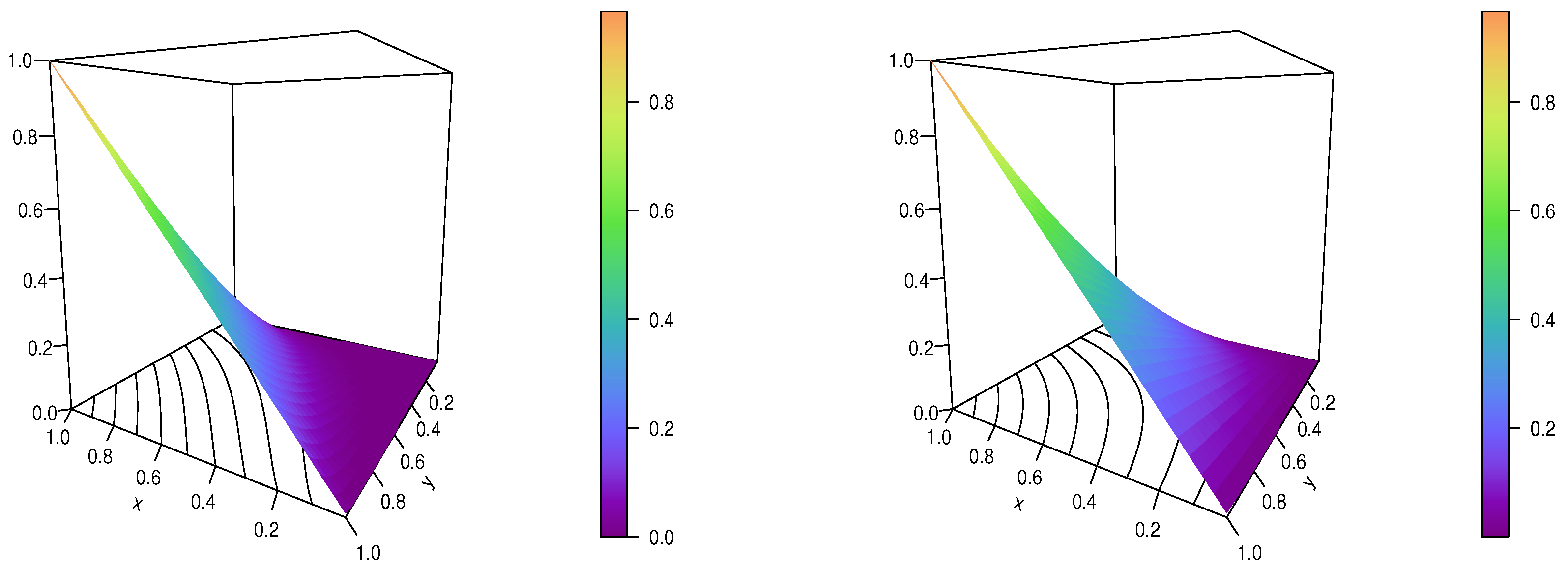
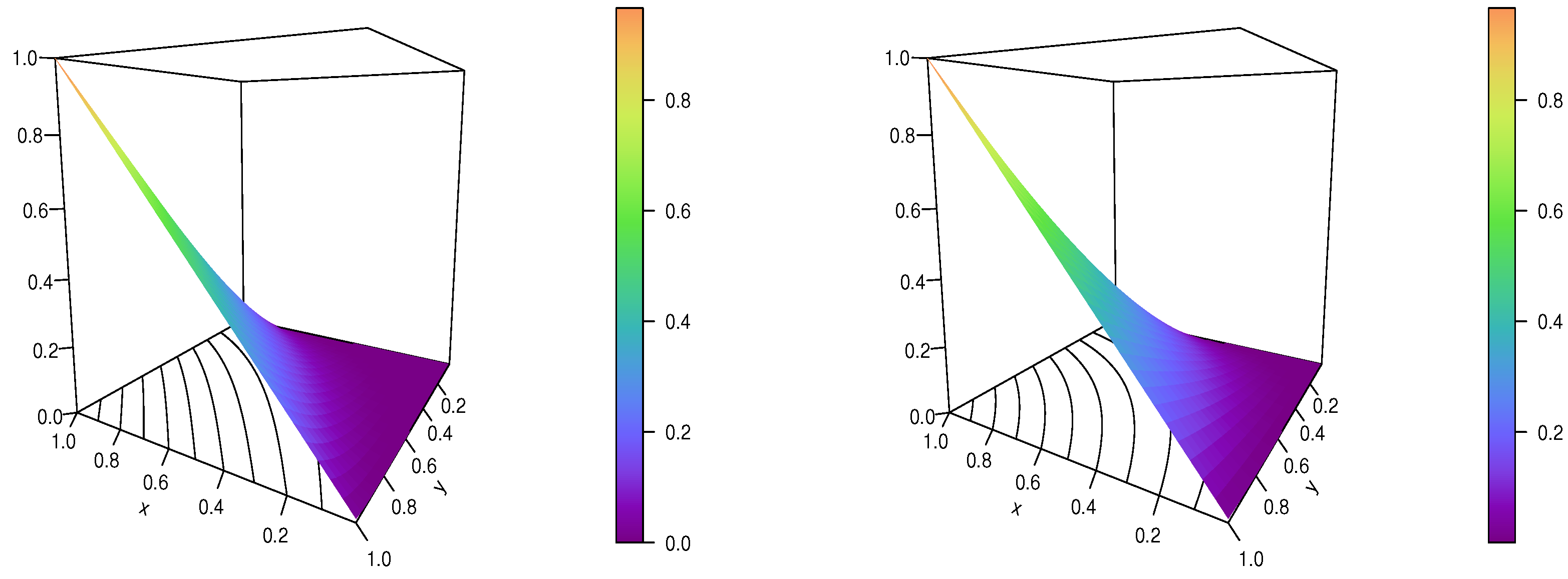
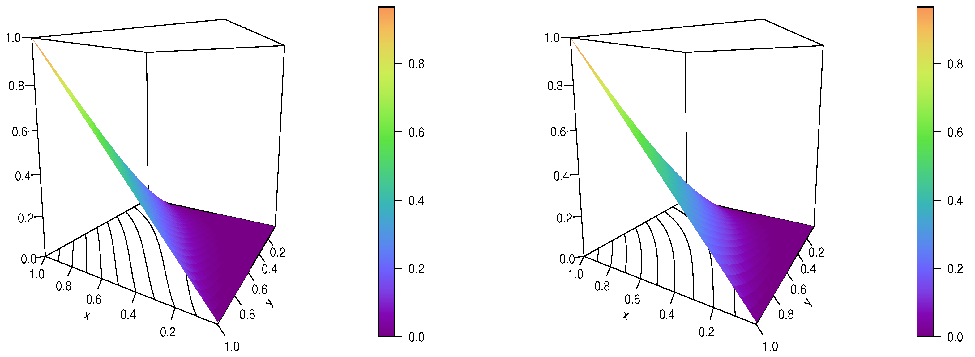
For illustrative purposes, Figure 2 and Figure 3 show some plots of the IP copula for selected admissible sets of parameter values.
It is evident from these figures that the IP copula is correct mathematically for the considered values. Moreover, depending on the values of and , a variety of deformations of the colored plan shape can be seen. The contour plots make this adaptability especially clear.
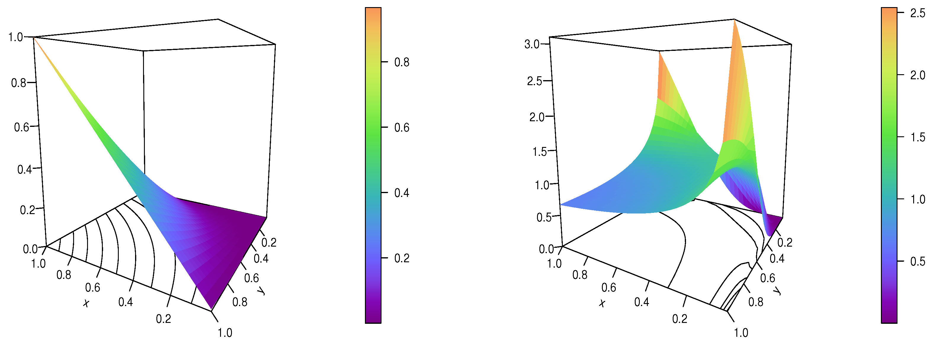
The IP copula density is determined using the following formula:
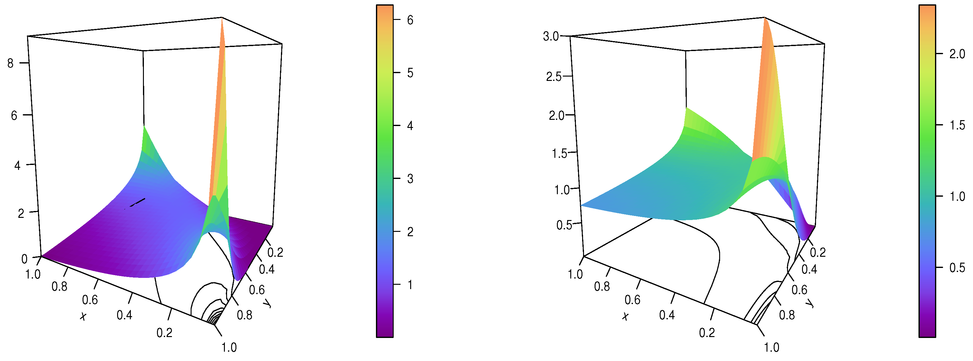
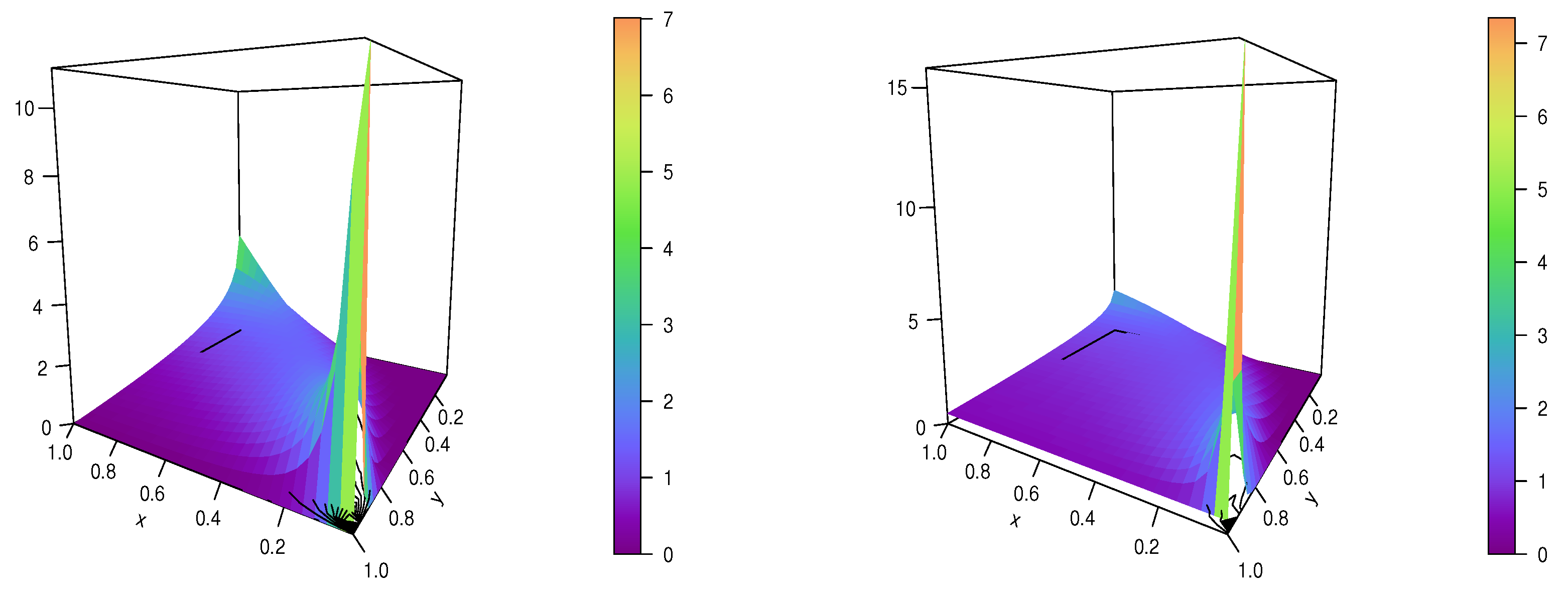
To comprehend the modeling capabilities of the IP copula, we may look at the shapes of its corresponding copula density. Thus, Figure 4 and Figure 5 display the IP copula density plots for various parameter values.
These figures reveal entirely distinct overall forms for the IP copula density, with a degenerate point at . Visually, the shapes are strongly influenced by and . The dependence flexibility is thus illustrated.
To end this portion, let us present some copulas that can be immediately derived from the IP copula. To begin, the x-flipping IP copula is specified as
The y-flipping IP copula is indicated as
Finally, the IP survival copula is given by
These copulas, which are new to the best of our knowledge, can be used as two-dimensional dependence models for data analysis. More information on the general formulas used for the flipping and survival approaches can be found in [5,25].
3.2. Fundamental Properties
In order to comprehend the modeling capability of the IP copula, this section establishes some fundamental properties of it. It is implicitly supposed that and . We recall that [3,4,5] contain most of the details about the upcoming concepts.
The exchangeability has already been mentioned; the IP copula is not exchangeable, except for , which corresponds to the independence copula case.
The IP copula is not Archimedean; the associative property is not satisfied in particular; for , for instance, we have and , which differ.
The IP copula is not radially symmetric, except for . Indeed, for , we can find such that .
We can apply the Fréchet–Hoeffding theorem, which guarantees that for any , we have , which can also be expressed as
For purposes unrelated to copulas, these inequalities may be of independent interest.
Let us set , with the parameter now being considered as a variable. Then, for any , and any and , we have
Thus, in this geometric mean sense, the IP copula is invariant. See [8] for more details on this invariance property.
Since, for any , , we have . Therefore, the IP copula is positively quadrant-dependent.
For any , we have
implying that is non-increasing with respect to . By setting , the following copula ordering holds: for any , we have .
Furthermore, for any , we have
implying that is non-increasing with respect to . By setting , the following copula ordering holds: for any , we have .
Let us now study the tail dependence of the IP copula. We have
Furthermore, we have
Due to the fact that , we draw the conclusion that the IP copula does not depend on the tail.
The medial correlation of the IP copula is calculated as
It is clearly negative.
Table 3 and Table 4 determine the numerical values of under the following configurations: { and } and { and }, respectively.
These tables show that for the particular configurations taken into account, we have . This range of values is quite good for this particular measure.
The Spearman rho of the IP copula is specified as
By integrating with respect to y, we obtain
It can be expressed for very specific values of the parameters. For instance, for (so ), the denominator of the integrated term is equal to 2, and we have . However, in full generality, the functional complexity of the integrated term is too high; the Spearman rho does not have a closed-form expression in terms of and .
Table 5 and Table 6 determine the numerical values of under the following configurations: { and } and { and }, respectively.
These tables show that the IP copula can only model negative dependence and that for the considered configurations, we have . This range of values is relatively large, which validates the IP copula for weak-to-moderate negative dependence.
The IP copula can serve as a generator of two-dimensional distributions. Indeed, by considering two unidimensional CDFs, say and , we define a new two-dimensional CDF as
In a two-dimensional lifetime data analysis scenario, one can consider lifetime baseline distributions. On this topic, we again refer to the survey in [26], and the references therein.
3.3. Statistical Study with Simulated Data
We now investigate the IP copula in a simulated data setting. Based on the available data, for the estimation of the parameters and , an efficient solution is the omnibus estimation method, as described in [28,29]. To present this method, let us consider observations drawn from a continuous random vector, such as . Thus, let n be the number of observations of this vector and be the observations representing the data. Then, the omnibus estimates (OEs) of and are determined as
where
,
and denotes the indicator function related to a set A. The accuracy of the omnibus estimation method is demonstrated in [28,29]. We now implement this method as an illustration.
For the first study, we generate pairs of data as follows: , where, for any , and are the observations of two independent random variables U and V that follow the exponential distribution with parameter 1. Then, the obtained OEs are and , which are clearly admissible. Based on these estimates, we define the estimated IP copula density as
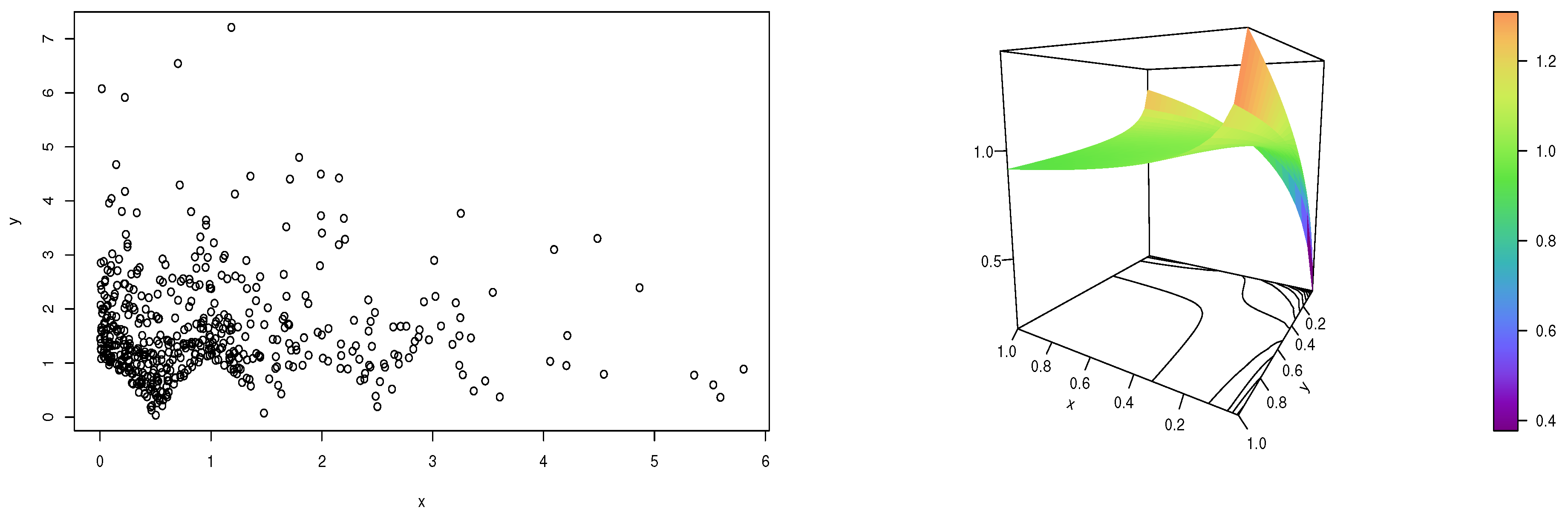
Figure 6 displays the scatter plot of the data and the estimated function.
This figure thus illustrates the functional print of the dependence structure behind the considered data.
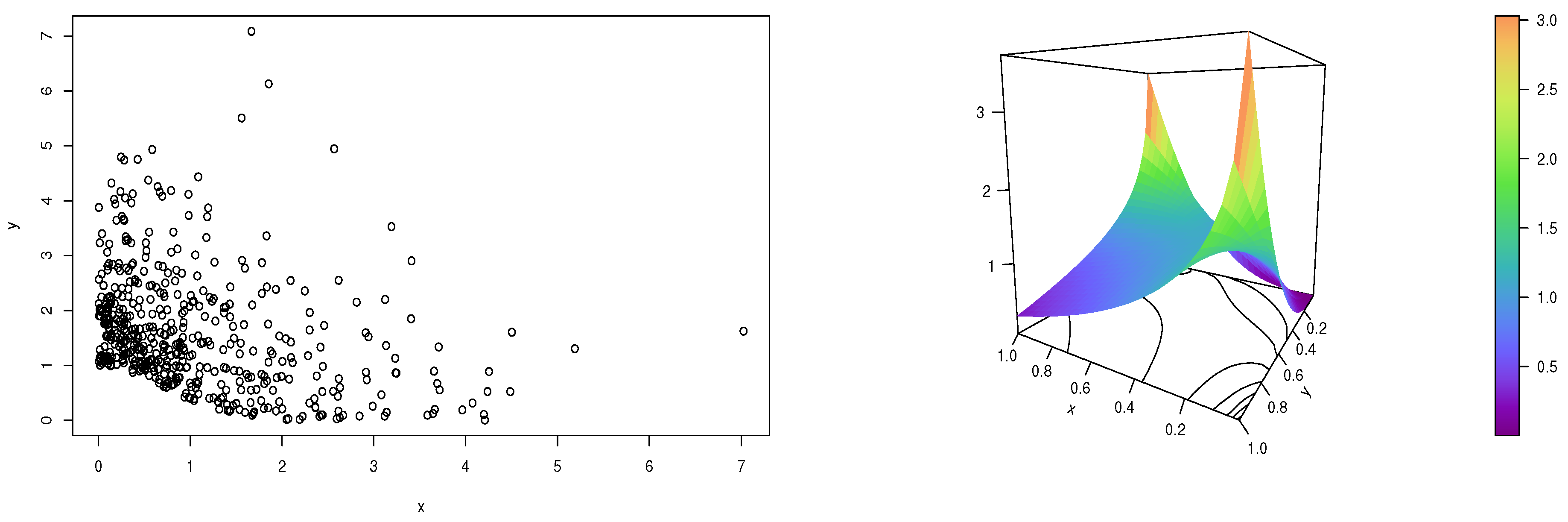
A second simulated study is now performed with other kinds of data. We generate pairs of data as follows: , where, for any , and are still the observations of two independent random variables U and V that follow the exponential distribution with parameter 1. In this experiment, the obtained OEs are and , which are clearly admissible. Based on these estimates, we consider the estimated IP copula density with the substitution technique as described above.
Figure 7 displays the scatter plot of the data and the estimated function.
This figure thus illustrates the functional print of the dependence structure behind the considered data. The differences in the OEs and in shapes in the estimated IP copula density prove the versatility of the IP copula and its ability to capture diverse structures of dependence.
This simulated work can be viewed as the first step for the application of the IP copula to real-data sets.
4. On Two Intriguing OVP Copulas
We complete this study with the presentation of two intriguing OVP copulas, completely different from those described above. They are intriguing because of their original definition, which is so far beyond the standard and has a certain degree of complexity from a mathematical viewpoint. As main features, the first proposed copula uses the term in power , which seems unique in the literature, and the second copula mixes various powers of x, including in the power of the main term. Some connections to the Ali–Mikhail–Haq copula are highlighted for this one. To the best of our knowledge, they are completely new.
4.1. Intriguing OVP Copula 1
The next result presents the first intriguing copula.
Proposition 6.
The following two-dimensional OVP function is a copula:
(no parameters are involved).
Proof.
The proof consists in demonstrating that satisfies the points (I), (II), and (III) of Definition 1.
- Proof
- for (I) For any , we haveFor any , with the use of limits, we obtainThis ends this portion of the proof.
- Proof
- for (II) For any , we haveFor any , we haveThis ends this portion of the proof.
- Proof
- for (III) After differentiation with the usual rules and several simplifications and factorizations, for any , we findWe aim to prove that this function is non-negative. For any , since and , owing to the following logarithmic inequality: for , we haveUsing , we getSince and , we finally obtainThis ends this portion of the proof.
The proof of Proposition 6 ends. □
For the purpose of this study, the copula defined in Equation (6) is named the intriguing 1 (Int1) copula.
Some functions and properties related to the Int1 copula are listed below. To begin, the Int1 copula density is given by
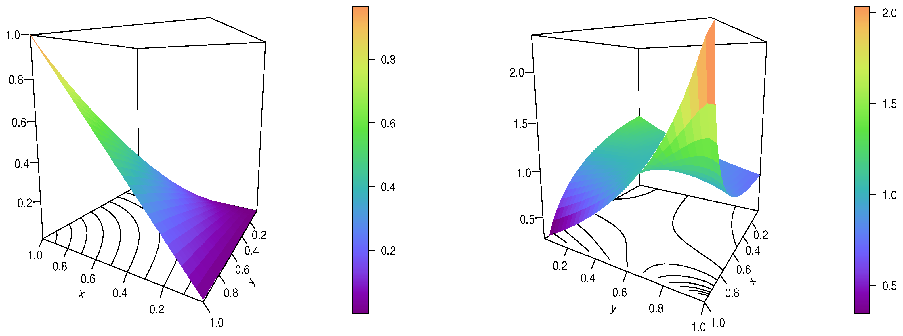
For a visual analysis, the Int1 copula and Int1 copula density are represented in Figure 8.
This figure reveals some shapes of the Int1 copula and Int1 copula density, also illustrating their validity in the mathematical sense; it is clear that , , etc.
Among the new copulas that can be derived from the Int1 copula are the x-flipping Int1 copula, specified as
the y-flipping Int1 copula indicated as
and the Int1 survival copula given by
All these copulas can serve as two-dimensional dependence models in two-dimensional data analysis scenarios.
For the main properties, the Int1 copula is (obviously) free of parameters, not exchangeable, not radially symmetric, not Archimedean, its medial correlation is equal to , and its Spearman rho is equal to
As a last result, we may also mention the Fréchet–Hoeffding theorem that asserts that for any , so
This result innovates from a multidimensional (or multivariate) analysis viewpoint.
The Int1 copula is of mathematical interest because of its very original OVP definition. However, because there are no tuning parameters, it suffers from a lack of flexibility in a practical scenario. Several techniques to add parameters are possible, but we drop this aspect here.
The next part proposes another intriguing OVP copula that has the feature of depending on two tuning parameters, among others.
4.2. Intriguing OVP Copula 2
The next result presents the second intriguing copula.
Proposition 7.
Let . Then, for and , the following two-dimensional OVP function is a copula:
Proof.
The proof consists in demonstrating that satisfies the points (I), (II), and (III) of Definition 1.
- Proof
- for (I) For any , since , and , we haveFor any implying that , , and , we haveThis ends this portion of the proof.
- Proof
- for (II) For any , we haveFor any , we have
- Proof
- for (III) After differentiation with the standard rules and several simplifications and factorizations, for any , we findSince, for , it is clear that the main multiplicative term is non-negative, and we have . Owing to and the following logarithmic inequality: for , we haveSince , , we have , and . Therefore, for any , the term in curly brackets is non-negative, and we finally have
The proof of Proposition 7 ends. □
For the purpose of this study, the copula defined in Equation (7) is named the intriguing 2 (Int2) copula. Our result excludes the case , since we focus on copulas of the OVP type, but we can prove that in this case, the Int2 copula is still valid for ; the case corresponds to the independence copula.
Furthermore, one can notice that for , it can be expressed as , where is the Ali–Mikhail–Haq copula given by Equation (5).
Some functions and properties related to the Int2 copula are listed below. To begin, the Int2 copula density is given by
For a visual analysis, the Int2 copula and Int2 copula density are represented in Figure 9 and Figure 10 for {} and { and }, respectively.
These figures demonstrate the flexibility of the Int2 copula and Int2 copula density according to the values of and .
Thanks to the flipping and survival approaches, the following copulas can be deduced: the x-flipping Int2 copula is given by
the y-flipping Int2 copula is specified as
and the Int2 survival copula is indicated as
All these copulas can serve as two-dimensional dependence models in various data analysis scenarios involving two quantitative variables.
For the main properties, we claim that the Int2 is not exchangeable, not radially symmetric, not Archimedean, and its medial correlation is equal to . The Spearman rho of the Int2 copula has the following complex integral form:
No closed-form expressions were found. In order to get an idea of its range of values, under the special configuration { with }, Table 7 presents some of its values.
From this table, we see that the Int2 copula can model negative dependence with a wide range of values; for the considered configuration, which is certainly not optimal, we find . It is thus of interest to analyze the dependence of two quantitative variables that are compatible with such features.
As a last result, we may also mention the Fréchet–Hoeffding theorem that implies that for any , so
To our knowledge, these inequalities are new, so they have potential interest.
5. Conclusions
This article focused on the full theory of underexplored copulas with one-variable power, i.e., of the form , where denotes a specific function. In the main result, we identified the precise assumptions required on to validate such copulas. Based on the flipping and survival strategies, some additional general copulas were described. Numerous examples of function depending on two or three parameters were given. In particular, we demonstrated that our assumptions and well-known truncated lifetime distributions have a close relationship. In order to emphasize the significance of our findings, we focused on a specific two-parameter, one-variable-power copula that combined the definition of the independence copula with the intriguing copula defined as . Its different shapes, associated functions, and various correlation features were revealed. The theory was rendered in numerical tables and graphics to make it less abstract. A short statistical work was given to show how the involved parameters can be estimated based on data. Two new intriguing one-variable-power copulas beyond the thought-of general form were finally presented and studied. A new one-variable-power extension of the so-called Ali–Mikhail–Haq copula can be seen in the second one. Additionally, they have appealing correlation properties that can be used in a variety of statistical contexts, such as the modeling of various claim types, payment and incurred loss data, cross-industry- and cross-breach-type structures for monthly cyber losses, the mortality of some countries, etc.
This article lays the theoretical groundwork for further exploration of one-variable-power copulas, including the extensions to a higher dimension and applications to the analysis of contemporary data in a two-dimensional setting. These aspects are postponed for future work.
Funding
This research received no external funding.
Data Availability Statement
Not applicable.
Acknowledgments
The author would like to thank the the four reviewers for their thorough and constructive comments on the paper.
Conflicts of Interest
The author declares no conflict of interest.
References
- Sklar, A. Fonctions de répartition à n dimensions et leurs marges. Publ. L’Institut Stat. L’UniversitÉ Paris 1959, 8, 229–231. [Google Scholar]
- Sklar, A. Random variables, joint distribution functions, and copulas. Kybernetika 1973, 9, 449–460. [Google Scholar]
- Durante, F.; Sempi, C. Principles of Copula Theory; CRS Press: Boca Raton, FL, USA, 2016. [Google Scholar]
- Joe, H. Dependence Modeling with Copulas; CRS Press: Boca Raton, FL, USA, 2015. [Google Scholar]
- Nelsen, R. An Introduction to Copulas, 2nd ed.; Springer Science+Business Media, Inc.: Berlin/Heidelberg, Germany, 2006. [Google Scholar]
- Chesneau, C. A collection of new trigonometric- and hyperbolic-FGM-type copulas. AppliedMath 2023, 3, 147–174. [Google Scholar] [CrossRef]
- Cuadras, C.M.; Diaz, W.; Salvo-Garrido, S. Two generalized bivariate FGM distributions and rank reduction. Commun. -Stat.-Theory Methods 2020, 49, 5639–5665. [Google Scholar] [CrossRef]
- Diaz, W.; Cuadras, C.M. An extension of the Gumbel-Barnett family of copulas. Metrika 2022, 85, 913–926. [Google Scholar] [CrossRef]
- Dolati, A.; Úbeda-Flores, M. Constructing copulas by means of pairs of order statistics. Kybernetika 2009, 45, 992–1002. [Google Scholar]
- El Ktaibi, F.; Bentoumi, R.; Sottocornola, N.; Mesfioui, M. Bivariate copulas based on counter-monotonic shock method. Risks 2022, 10, 202. [Google Scholar] [CrossRef]
- Huang, J.S.; Kotz, S. Modifications of the Farlie-Gumbel-Morgenstern distributions. A tough hill to climb. Metrika 1999, 49, 135–145. [Google Scholar] [CrossRef]
- Chesneau, C. On new types of multivariate trigonometric copulas. AppliedMath 2021, 1, 3–17. [Google Scholar] [CrossRef]
- Lai, C.D.; Xie, M. A new family of positive quadrant dependent bivariate distributions. Stat. Probab. Lett. 2000, 46, 359–364. [Google Scholar] [CrossRef]
- Manstavičius, M.; Bagdonas, G. A class of bivariate independence copula transformations. Fuzzy Sets Syst. 2022, 428, 58–79. [Google Scholar] [CrossRef]
- Chesneau, C. On new three- and two-dimensional ratio-power copulas. Comput. J. Math. Stat. Sci. 2023, 2, 106–122. [Google Scholar] [CrossRef]
- Saali, T.; Mesfioui, M.; Shabri, A. Multivariate extension of Raftery copula. Mathematics 2023, 11, 414. [Google Scholar] [CrossRef]
- Bayramoglu, K.; Bayramoglu, I. Baker—Lin-Huang type bivariate distributions based on order statistics. Commun.-Stat.–Theory Methods 2014, 43, 10–12. [Google Scholar] [CrossRef]
- Bekrizadeh, H.; Parham, G.; Jamshidi, B. A new asymmetric class of bivariate copulas for modeling dependence. Commun. Stat.-Simul. Comput. 2017, 46, 5594–5609. [Google Scholar] [CrossRef]
- Chesneau, C. Theoretical contributions to three generalized versions of the Celebioglu-Cuadras copula. Analytics 2023, 2, 31–54. [Google Scholar] [CrossRef]
- Celebioglu, S. A way of generating comprehensive copulas. J. Inst. Sci. Technol. 1997, 10, 57–61. [Google Scholar]
- Cuadras, C.M. Constructing copula functions with weighted geometric means. J. Stat. Plan. Inference 2009, 139, 3766–3772. [Google Scholar] [CrossRef]
- Eling, M.; Jung, K. Copula approaches for modeling cross-sectional dependence of data breach losses. Insur. Econ. 2018, 82, 167–180. [Google Scholar] [CrossRef]
- Erhardt, V.; Czado, C. Modeling dependent yearly claim totals including zero claims in private health insurance. Scand. Actuar. J. 2012, 2012, 106–129. [Google Scholar] [CrossRef]
- Shi, P.; Valdez, E.A. Multivariate negative binomial models for insurance claim counts. Insur. Math. Econ. 2014, 55, 18–29. [Google Scholar] [CrossRef]
- De Baets, B.; De Meyer, H.; Kalická, J.; Mesiar, R. Flipping and cyclic shifting of binary aggregation functions. Fuzzy Sets Syst. 2009, 160, 752–765. [Google Scholar] [CrossRef]
- Taketomi, N.; Yamamoto, K.; Chesneau, C.; Emura, T. Parametric distributions for survival and reliability analyses, a review and historical sketch. Mathematics 2022, 10, 3907. [Google Scholar] [CrossRef]
- R Core Team. R: A Language and Environment for Statistical Computing. Vienna, Austria. 2016. Available online: https://www.R-project.org/ (accessed on 3 January 2023).
- Genest, C.; Ghoudi, K.; Rivest, L.P. A semiparametric estimation procedure of dependence parameters in multivariate families of distributions. Biometrika 1995, 82, 543–552. [Google Scholar] [CrossRef]
- Silvapulle, P.; Kim, G.; Silvapulle, M.J. Robustness of a semiparametric estimator of a copula. Econom. Soc. 2004 Australas. Meet. 2004, 2004, 317. [Google Scholar]
Figure 1.
Plots of the TE copula for (left) and (right).

Figure 2.
Plots of the IP copula for and (left) and (right).

Figure 3.
Plots of the IP copula for and (left) and (right).

Figure 4.
Plots of the IP copula density for and (left) and (right).

Figure 5.
Plots of the IP copula density for and (left) and (right).

Figure 6.
Scatter plot of the data (left) and plot of the estimated IP copula density (right).

Figure 7.
Scatter plot of the data (left) and plot of the estimated IP copula density (right).

Figure 8.
Plots of the Int1 copula (left) and the Int1 copula density (right).

Figure 9.
Plots of the Int2 copula (left) and the Int2 copula density (right) for .

Figure 10.
Plots of the Int2 copula (left) and the Int2 copula density (right) for and .


Table 1.
Copulas derived from Theorem 1 and Lemma 1.
| Name | Abbreviation | Copula C(x,y) | Conditions | New |
|---|---|---|---|---|
| Power | P | , , | Yes | |
| Exponential-power | EP | , | Yes | |
| Sine | S | , , | Yes | |
| Logarithmic | L | No | ||
| Inverse-power | IP | , | Yes |
Table 2.
Copulas derived from Theorem 1 and Lemma 2.
| Name | Abbreviation | Copula | Conditions |
|---|---|---|---|
| Truncated exponential | TE | ||
| Truncated exponential–logarithmic | TEL | , | |
| Truncated Lomax | TL | , | |
| Truncated half-normal | THN |
Table 3.
Numerical values of for and .
| 0 | 0.1 | 0.2 | 0.3 | 0.4 | 0.5 | 0.6 | 0.7 | 0.8 | 0.9 | 1.0 | |
|---|---|---|---|---|---|---|---|---|---|---|---|
| 0 | −0.067 | −0.1294 | −0.1877 | −0.2421 | −0.2929 | −0.3402 | −0.3844 | −0.4257 | −0.4641 | −0.5 |
Table 4.
Numerical values of for and .
| 0 | 0.2 | 0.4 | 0.6 | 0.8 | 1.0 | 1.2 | 1.4 | 1.6 | 1.8 | 2.0 | |
|---|---|---|---|---|---|---|---|---|---|---|---|
| 0 | −0.0558 | −0.1085 | −0.1582 | −0.2496 | −0.2914 | −0.331 | −0.3683 | −0.4036 | −0.4369 |
Table 5.
Numerical values of for and .
| 0 | 0.1 | 0.2 | 0.3 | 0.4 | 0.5 | 0.6 | 0.7 | 0.8 | 0.9 | 1.0 | |
|---|---|---|---|---|---|---|---|---|---|---|---|
| 0 | −0.1221 | −0.2179 | −0.2992 | −0.3706 | −0.4344 | −0.4923 | −0.5453 | −0.5943 | −0.6397 | −0.6822 |
Table 6.
Numerical values of for and .
| 0 | 0.2 | 0.4 | 0.6 | 0.8 | 1.0 | 1.2 | 1.4 | 1.6 | 1.8 | 2.0 | |
|---|---|---|---|---|---|---|---|---|---|---|---|
| 0 | −0.0918 | −0.1713 | −0.2421 | −0.306 | −0.3645 | −0.4184 | −0.4684 | −0.5151 | −0.5588 | −0.6 |
Table 7.
Numerical values for with and .
| 0 | 0.2 | 0.4 | 0.6 | 0.8 | 1.0 | 1.2 | 1.4 | 1.6 | 1.8 | 2.0 | |
|---|---|---|---|---|---|---|---|---|---|---|---|
| 0 | −0.0981 | −0.1919 | −0.281 | −0.3654 | −0.4453 | −0.5209 | −0.5926 | −0.6605 | −0.725 | −0.7862 |
Disclaimer/Publisher’s Note: The statements, opinions and data contained in all publications are solely those of the individual author(s) and contributor(s) and not of MDPI and/or the editor(s). MDPI and/or the editor(s) disclaim responsibility for any injury to people or property resulting from any ideas, methods, instructions or products referred to in the content. |
© 2023 by the author. Licensee MDPI, Basel, Switzerland. This article is an open access article distributed under the terms and conditions of the Creative Commons Attribution (CC BY) license (https://creativecommons.org/licenses/by/4.0/).
Share and Cite
MDPI and ACS Style
Chesneau, C. Theoretical Validation of New Two-Dimensional One-Variable-Power Copulas. Axioms 2023, 12, 392. https://doi.org/10.3390/axioms12040392
AMA Style
Chesneau C. Theoretical Validation of New Two-Dimensional One-Variable-Power Copulas. Axioms. 2023; 12(4):392. https://doi.org/10.3390/axioms12040392
Chicago/Turabian StyleChesneau, Christophe. 2023. "Theoretical Validation of New Two-Dimensional One-Variable-Power Copulas" Axioms 12, no. 4: 392. https://doi.org/10.3390/axioms12040392
Note that from the first issue of 2016, this journal uses article numbers instead of page numbers. See further details here.