Dynamics of a Double-Impulsive Control Model of Integrated Pest Management Using Perturbation Methods and Floquet Theory

Abstract

We formulate an integrated pest management model to control natural pests of the crop through the periodic application of biopesticide and chemical pesticides. In a theoretical analysis of the system pest eradication, a periodic solution is found and established. All the system variables are proved to be bounded. Our main goal is then to ensure that pesticides are optimized, in terms of pesticide concentration and pesticide application frequency, and that the optimum combination of pesticides is found to provide the most benefit to the crop. By using Floquet theory and the small amplitude perturbation method, we prove that the pest eradication periodic solution is locally and globally stable. The acquired results establish a threshold time limit for the impulsive release of various controls as well as some valid theoretical conclusions for effective pest management. Furthermore, after a numerical comparison, we conclude that integrated pest management is more effective than single biological or chemical controls. Finally, we illustrate the analytical results through numerical simulations.

1. Introduction

In today’s farming systems, a variety of approaches are used for pest control. Maintaining high output while guaranteeing sustainability is crucial for the entire agriculture sector. Since the beginning of human civilization, insect and pest control has been one of the most significant difficulties in the agricultural sector [1,2]. Every day, people come up with fresh ideas for equipment and tactics to use in their fight against pests. As a result of human efforts to manage pests, our natural ecology and nature are on the verge of extinction [3].

Chemical controls are less expensive to implement, yet they result in significant environmental damage [4,5,6]. On the other hand, biological controls are more costly to implement but have less environmental impact [7]. However, frequently, the use of a single control method is not beneficial to control pest resistance and preserve environmental quality [8,9]. In order to reduce insect populations below economic levels, integrated pest management (IPM), a safer and more effective method, was developed. IPM is used for a variety of agronomic crops and is now widely used as an economical and environment-friendly pest control method in several nations [8,9,10]. When the ecological cost of management is added to the economic price of controls, a combination of chemical and biological controls yields a superior result when they are used with proper rate and with tolerable intervals. Modeling of this phenomenon leads naturally to the use of impulsive differential equations [11,12].

Many researchers have designed mathematical models for pest management through control strategies, some of which promote chemical agents [4,7], some advocate the use of biological agents to impose a total solution of pest and disease [1,2,10,13,14,15], and some researchers use both the chemical and biopesticides in their mathematical models [5,16,17,18]. Mathematical-model-based works using impulsive differential equations are also available in the literature, as already mentioned [19,20,21,22,23,24,25,26]. Recently, Li, Huang, and Liu proposed a pest management model to simulate the application of pesticides and build a pesticide function with residual and delayed effects of pesticides, proposing pest management with pollutant emission [27]. Liu et al. constructed a mathematical model for pest control in which susceptible and infected pests are separated from the pest population and only susceptible pests are harmful to crops [28]. They weighed the two approaches of spraying pesticides and releasing diseased pests and natural enemies to control vulnerable pests when completing their task. Alzabut established a mathematical model based on the sense of biological survey in the field of agriculture, and introduced various control methods to determine how to protect the crops from destructive pests [29]. In [24], an integrated pest management model using impulsive differential equations was proposed and analyzed for Jatropha curcas using the release of infective pests and spraying of chemical pesticides. The existence and stability of susceptible pest-eradication solutions were analyzed using Floquet theory and the small amplitude perturbation method. To the best of our knowledge, all available articles deal with single-impulse differential equation models where the stability analysis of the periodic pest extinction solution is obtained by the Floquet theory, the method of small amplitude perturbation, and the comparison theorem. However, none of the prior research available in the literature employs the concentration of chemical pesticides as a system variable as we do here. Moreover, in our study, we spray biological and chemical pesticides at two different time intervals, simultaneously varying the time period.

Pest control models using a single impulse are available (see, e.g., [30]), but using double-impulsive controls is rare [31,32]. The authors of [31] took a predator population along with biopesticides in an impulsive periodic way for the control of crop pests. The authors of [32] proposed a predator–prey model with disease in the prey and investigated it for the purpose of integrated pest management. The permanence of the system and global stability of the susceptible pest-eradication periodic solution were shown by means of the released amounts of infective prey and predator. In contrast, here, impulses on both chemical and biopesticides were assumed in the formulation of the mathematical model for crop pest management.

Our use of the concentration profile of the chemical pesticide as a model variable is a novel approach. We demonstrated the dynamics using both the chemical and biological pesticides in the system in an impulsive way, which is, to the best of our knowledge, a novel concept in crop pest control. The proposed double-impulsive system was analyzed with proper analytical methods, namely, using Floquet theory and the perturbation method.

Floquet theory is a powerful mathematical tool for analyzing periodic systems, and it can be extended to impulsive models with periodic impulses. In impulsive models, the system’s behavior is characterized by a sequence of discrete impulses applied at regular intervals. These impulses may arise in many practical scenarios, including electrical circuits, control systems, and biological systems. Floquet theory provides a robust framework for analyzing and designing control strategies for impulsive models with periodic impulses. One can analyze the stability of the impulsive system by examining the eigenvalues of the Floquet matrix [33]. In our analysis, we utilize small amplitude perturbation techniques and Floquet theory and obtain some valid theoretical results for successful management of pests. Moreover, we also establish the threshold time limit for the impulsive release of control agents. Our approach for using the Floquet theory is novel. Additionally, we examined the dynamics of the system for biological and chemical pesticides used as a sole control measure.

The paper is organized as follows. In Section 2, we derive the model by using impulsive differential equations for capturing the IPM system dynamics, taking plant, pest, virus, and chemical pesticide as model variables. The mathematical analysis of the model is then discussed in Section 3, which contains three subsections. In Section 3.1, we determine susceptible pest-eradication periodic solutions and check the feasibility–boundedness of the system variables discussed in Section 3.2. The local and global stability conditions around the susceptible pest-eradication periodic solutions are explored in Section 3.3. In Section 4, we exhibit our mathematical results through numerical simulations. Finally, in Section 5, we provide a discussion on the three types of control strategies: spraying chemical pesticide only, impulsively incorporating of infected pest only, and integrated control with a fixed and a variable impulse period, to make the final conclusion.

2. Derivation of the Impulsive Control Model

The following assumptions are taken to formulate the desired model: the crop plant and susceptible pest populations are denoted by x and y, respectively, and we denote z as the infected pest population.

Due to the finite size of a crop field, which, however, may be large, we assume logistic growth for the biomass of the crop, with net growth rate r and carrying capacity k. Crops become affected by pests, thereby causing considerable crop reduction.

Let $\alpha$ be the contact rate between crop and susceptible pest; let $v\left(t\right)$ be the biopesticide (virus); and s be the concentration of chemical pesticide. A virus infects the susceptible pest at a rate, $\lambda$. The chemical pesticide kills the susceptible and infected pests at the rates $m_1$ and $m_2$, respectively. Parameters $c_1$ and $c_2$ are the conversion factors of susceptible and infected pests, respectively, due to consumption of crop; d and $d+\delta$ are the mortality rates of susceptible and infected pest, respectively; $\theta$ is the virus replication rate; and $\gamma$ is the lysis rate of the virus. Finally, we introduce a periodic application of biopesticide and chemical pesticide with different time intervals.

Based on the above assumptions, the desired impulsive system for integrated pest management is given as

$$\left\{\begin{array}{cc}{\displaystyle \frac{dx}{dt}=rx\left(1-\frac{x}{k}\right)-\alpha xy-\varphi \alpha xz,}\hfill & t\ne (n{\tau }_1,n{\tau }_2),\hfill \\ {\displaystyle \frac{dy}{dt}=c_1\alpha xy-\lambda yv-dy-m_{1}sy,}\hfill & t\ne (n{\tau }_1,n{\tau }_2),\hfill \\ {\displaystyle \frac{dz}{dt}=c_2\varphi \alpha xz+\lambda yv-(d+\delta )z-m_{2}sz,}\hfill & t\ne (n{\tau }_1,n{\tau }_2),\hfill \\ {\displaystyle \frac{dv}{dt}=\theta (d+\delta )z-\gamma v,}\hfill & t\ne (n{\tau }_1,n{\tau }_2),\hfill \\ {\displaystyle \frac{ds}{dt}=-\mu s,}\hfill & t\ne (n{\tau }_1,n{\tau }_2),\hfill \\ {\displaystyle v\left(t^{+}\right)=v\left(t^{-}\right)+v_i,}\hfill & t=n{\tau }_1,\hfill \\ {\displaystyle s\left(t^{+}\right)=s\left(t^{-}\right)+s_i,}\hfill & t=n{\tau }_2,\hfill \end{array}\right.$$

(1)

where $v_i$ and $s_i$ are the strength of biopesticide and chemical pesticide application in the system at $t=n{\tau }_1$ and $t=n{\tau }_2$, respectively; $n=0,1,2,3,\dots$, where ${\tau }_1$ and ${\tau }_2$ are the time periods. Here, $v\left(t^{-}\right)$ and $s\left(t^{-}\right)$ are the strength of biopesticide and chemical pesticide before the periodic input, and $v\left(t^{+}\right)$ and $s\left(t^{+}\right)$ are the strength of biopesticide and chemical pesticide after the periodic input.

In the impulsive model (1), we assumed the concentration of chemical pesticide as a model population, which is realistic and a novel idea. We use two different impulse intervals for two control agents (biopesticide and chemical pesticide) that will be analyzed both analytically and numerically. We proceed by analyzing the dynamics of model (1) by discussing the existence of equilibria with their stability.

3. Dynamics of the Impulsive Model

In this section, we analyze the boundedness of the solutions of system (1), we find out its pest-eradication steady state, and we analyze the local and global stability. Finally, we discuss the permanence of the impulsive system.

3.1. Boundedness of the Model Variables

Let $V\left(t\right)=x\left(t\right)+y\left(t\right)+z\left(t\right)+v\left(t\right)+s\left(t\right)$ and

$$\begin{array}{ccc}\hfill \frac{dV}{dt}+mV& \le & \left(rx+mx-\frac{r{x}^2}{k}\right)-(1-c_1)\alpha xy-(1-c_2)\varphi \alpha xz-\{(d-m\}y\hfill \\ & & -\left\{\right(1-\theta \left)\right(d+\delta )-m\}z-(\gamma -m)v-(\mu -m)s.\hfill \end{array}$$

Now, let us define $m=min\{d,\gamma ,\mu ,(d+\delta \left)\right(1-\theta \left)\right\}$. As $0<c_1,c_2,\theta <1$, then $1-c_1>0$, $1-c_2>0$, and $1-\theta >0$, so we can write that

$$\begin{array}{ccc}\hfill \frac{dV\left(t\right)}{dt}+mV\left(t\right)& \le & M_0,\hfill \end{array}$$

(2)

where ${\displaystyle \frac{k{(m+r)}^2}{4r}=M_0}$. At $t=n{\tau }_1$, we have

$$\begin{array}{c}\hfill V\left(n{\tau }_1^{+}\right)\le V\left(n{\tau }_1\right)+v_i.\end{array}$$

(3)

By the comparison theorem, for $t\ge 0$ we have

$$\begin{array}{ccc}\hfill V\left(t\right)& \le & V\left(0\right)e^{-mt}+\frac{M_0(1-e^{-mt})}{m}+v_i\frac{e^{-m(t-{\tau }_1)}}{1-e^{m{\tau }_1}}+v_i\frac{e^{m{\tau }_1}}{e^{m{\tau }_1}-1}\hfill \\ & \to & \frac{M_0}{m}+v_i\frac{e^{m{\tau }_1}}{e^{m{\tau }_1}-1}\mathrm{as}t\to \infty .\hfill \end{array}$$

(4)

When $t=n{\tau }_2$,

$$\begin{array}{c}\hfill V\left(n{\tau }_2^{+}\right)\le V\left(n{\tau }_2\right)+v_i\end{array}$$

(5)

and from the comparison theorem it follows that

$$\begin{array}{ccc}\hfill V\left(t\right)& \le & V\left(0\right)e^{-mt}+\frac{M_0(1-e^{-mt})}{m}+v_i\frac{e^{-m(t-{\tau }_2)}}{1-e^{m{\tau }_2}}+v_i\frac{e^{m{\tau }_2}}{e^{m{\tau }_2}-1}\hfill \\ & \to & \frac{M_0}{m}+v_i\frac{e^{m{\tau }_2}}{e^{m{\tau }_2}-1}\mathrm{as}t\to \infty .\hfill \end{array}$$

(6)

Thus, $V\left(t\right)$ is uniformly bounded and there exists a positive constant $M>0$ such that $x\left(t\right)\le M$, $y\left(t\right)\le M$, $z\left(t\right)\le M$, $v\left(t\right)\le M$, and $s\left(t\right)\le M$ for all t.

From the above discussion, we have the following theorem.

Theorem 1.

For the impulsive system (1), there exists a positive constant M such that $x\left(t\right)\le M$, $y\left(t\right)\le M$, $z\left(t\right)\le M$, $v\left(t\right)\le M$, and $s\left(t\right)\le M$ for all t.

For non-negative solutions, the following lemma follows from [13].

Lemma 1.

Let $X\left(t\right)$ be a solution of the impulsive system (1) with $X\left(0^{+}\right)\ge 0$. Then $X\left(t\right)\ge 0$ for all $t>0$.

3.2. Existence of the Pest-Free Periodic Orbit

Since both pests are assumed to be harmful for crops, we discuss stability at infected and susceptible pest-eradication solutions of the system when $y=0$ and $z=0$, $t\ne (n{\tau }_1,n{\tau }_2)$, and the linear forms of the fourth and fifth equation of (1) are

$$\begin{array}{c}\hfill \frac{dv}{dt}=-\gamma v\mathrm{and}\frac{ds}{dt}=-\mu s,\end{array}$$

(7)

respectively. For an impulse control, we must have

$$\begin{array}{cc}\hfill v\left(t^{+}\right)& =v\left(t^{-}\right)+v_i,\mathrm{for}t={\tau }_1,\hfill \\ \hfill s\left(t^{+}\right)& =s\left(t^{-}\right)+s_i,\mathrm{for}t={\tau }_2.\hfill \end{array}$$

(8)

From (7) and (8) it is clear that v and s are independent of each other. Thus, the solution of Equation (7) can be given as follows:

$$\begin{array}{ccc}\hfill v\left(t\right)& =& \{v\left(0^{+}\right)-v^{\ast }\left(0^{+}\right)\}{e}^{-\gamma t}+v^{\ast }\left(t\right),fort\in ({\tau }_1,(n+1){\tau }_1],\hfill \\ \hfill s\left(t\right)& =& \{s\left(0^{+}\right)-s^{\ast }\left(0^{+}\right)\}{e}^{-\mu t}+s^{\ast }\left(t\right),for\in ({\tau }_2,(n+1){\tau }_2],\hfill \end{array}$$

(9)

where $v^{\ast }\left(t\right)$ and $s^{\ast }\left(t\right)$, the positive periodic solution of (7), are given by

$$\begin{array}{ccc}\hfill v^{\ast }\left(t\right)& =& \frac{v_i{e}^{-\gamma (t-n{\tau }_1)}}{1-e^{-\gamma {\tau }_1}},s^{\ast }\left(t\right)=\frac{s_i{e}^{-\mu (t-n{\tau }_2)}}{1-e^{-\mu {\tau }_2}},\hfill \end{array}$$

(10)

with initial values

$$v^{\ast }\left(0^{+}\right)=\frac{v_i}{1-e^{-\gamma {\tau }_1}},s^{\ast }\left(0^{+}\right)=\frac{s_i}{1-e^{-\mu {\tau }_2}}.$$

(11)

If $y\left(t\right)=0$ and $z\left(t\right)=0$, then the first equation of (1) is

$$\begin{array}{ccc}\hfill \frac{dx}{dt}& =& rx\left(1-\frac{x}{k}\right),\hfill \end{array}$$

(12)

which is a logistic equation, and its solution is

$$x\left(t\right)=\frac{kx\left(0\right)}{x\left(0\right)+(k-x\left(0\right))e^{rt}}\mathrm{for}t\ne (n{\tau }_1,n{\tau }_2).$$

(13)

Clearly, (13) has two equilibria, such as $x=0$ and $x=k$. Therefore, (1) has two pest-eradication solutions, $(0,0,0,v^{\ast },s^{\ast })$ and $(k,0,0,v^{\ast },s^{\ast })$. Obviously, at $x=0$ the system (13) is impossible from the perspective of ecology. For this reason, in the following subsection we study the stability for the system (1) at $E=(k,0,0,v^{\ast },s^{\ast })$.

3.3. Stability of the Pest-Free Periodic Solution

We establish the following theorem for the stability of the pest-free periodic orbit.

Theorem 2.

System (1) is both locally and globally stable around the pest-free periodic solution $E=(k,0,0,v^{\ast },s^{\ast })$ for the following:

(i)

Application of biopesticide and chemical pesticide with same time interval $t=n\tau$, provided that

$$\begin{array}{ccc}\hfill & & c_1\alpha -d-\frac{\lambda v_i{e}^{-\gamma (t-n\tau )}}{1-e^{-\gamma \tau }}-\frac{m_1{s}_i{e}^{-\mu (t-n\tau )}}{1-e^{-\mu \tau }}<0,\hfill \\ & & c_2\varphi k\alpha -(d+\delta )-\frac{m_2{s}_i{e}^{-\mu (t-n\tau )}}{1-e^{-\mu \tau }}<0;\hfill \end{array}$$

(14)

(ii)

Application of biopesticide with time interval $t=n{\tau }_1$ and chemical pesticide with time interval $t=n{\tau }_2$, i.e., for different time intervals, where ${\tau }_1\ne {\tau }_2$, provided that

$$\begin{array}{c}{c}_1\alpha -d-\frac{\lambda v_i{e}^{-\gamma (t-n{\tau }_1)}}{1-e^{-\gamma {\tau }_1}}<0,\\ c_2\varphi k\alpha -(d+\delta )<0,\\ c_1\alpha -d-\frac{m_1{s}_i{e}^{-\mu (t-n{\tau }_2)}}{1-e^{-\mu {\tau }_2}}<0.\end{array}$$

(15)

Proof. 

We need to prove the stability of the system in two cases:

(i) Application of chemical pesticide and biopesticide with same time interval;

(ii) Application of biopesticide and chemical pesticide with different time intervals.

(i) In this case, let $t=n{t}_1=n{t}_2=n\tau$. We discuss the stability of the system through the small amplitude perturbation method at the periodic solution $(k,0,0,v^{\ast },s^{\ast })$. Let

$$\begin{array}{ccc}\hfill & & x\left(t\right)=k+{ϵ}_1\left(t\right),y\left(t\right)={ϵ}_2\left(t\right),z\left(t\right)={ϵ}_3\left(t\right),\hfill \\ & & v\left(t\right)=v^{\ast }\left(t\right)+{ϵ}_4\left(t\right),s\left(t\right)=s^{\ast }\left(t\right)+{ϵ}_5\left(t\right).\hfill \end{array}$$

(16)

Here, ${ϵ}_1,{ϵ}_2,{ϵ}_3,{ϵ}_4$, and ${ϵ}_5$ denote small amplitude perturbations. Thus, the corresponding system of (1) at $(k,0,0,v^{\ast },s^{\ast })$ is given by

$$\begin{array}{ccc}\hfill \frac{d{ϵ}_1}{dt}& =& r\{k+{ϵ}_1\left(t\right)\}\left(1-\frac{k+{ϵ}_1\left(t\right)}{k}\right)-\alpha \{k+{ϵ}_1\left(t\right)\}{ϵ}_2\left(t\right)\hfill \\ & & -\varphi \alpha \{k+{ϵ}_1\left(t\right)\}{ϵ}_3\left(t\right),t\ne n\tau ,\hfill \\ \hfill \frac{d{ϵ}_2}{dt}& =& c_1\alpha \{k+{ϵ}_1\left(t\right)\}{ϵ}_2\left(t\right)-\lambda {ϵ}_2\left(t\right)\{v^{\ast }\left(t\right)+{ϵ}_4\left(t\right)\}\hfill \\ & & -d{ϵ}_2\left(t\right)-m_1\{s^{\ast }\left(t\right)+{ϵ}_5\left(t\right)\}{ϵ}_2\left(t\right),t\ne n\tau ,\hfill \\ \hfill \frac{d{ϵ}_3}{dt}& =& c_2\varphi \alpha \{k+{ϵ}_1\left(t\right)\}{ϵ}_3\left(t\right)+\lambda {ϵ}_2\left(t\right)\{v^{\ast }\left(t\right)+{ϵ}_4\left(t\right)\}-(d+\delta ){ϵ}_3\left(t\right)\hfill \\ & & -m_2\{s^{\ast }\left(t\right)+{ϵ}_5\left(t\right)\}{ϵ}_3\left(t\right),t\ne n\tau ,\hfill \\ \hfill \frac{d{ϵ}_4}{dt}& =& \theta (d+\delta ){ϵ}_3\left(t\right)-\gamma \{v^{\ast }\left(t\right)+{ϵ}_4\left(t\right)\},t\ne n\tau ,\hfill \\ \hfill \frac{d{ϵ}_5}{dt}& =& -\mu \{s^{\ast }\left(t\right)+{ϵ}_5\left(t\right)\},t\ne n\tau ,\hfill \\ \hfill ▵\{v^{\ast }\left(t\right)+{ϵ}_4\left(t\right)\}& =& v_i,t=n\tau ,\hfill \\ \hfill ▵\{s^{\ast }\left(t\right)+{ϵ}_5\left(t\right)\}& =& s_i,t=n\tau .\hfill \end{array}$$

(17)

Now, the linear system corresponding to the system (17) is given as

$$\begin{array}{ccc}\hfill \frac{d{ϵ}_1}{dt}& =& -r{ϵ}_1\left(t\right)-\alpha k{ϵ}_2\left(t\right)-\varphi \alpha k{ϵ}_3\left(t\right),t\ne n\tau ,\hfill \\ \hfill \frac{d{ϵ}_2}{dt}& =& c_1\alpha k{ϵ}_2\left(t\right)-\lambda {ϵ}_2\left(t\right)v^{\ast }\left(t\right)-d{ϵ}_2\left(t\right)-m_1{s}^{\ast }\left(t\right){ϵ}_2\left(t\right),t\ne n\tau ,\hfill \\ \hfill \frac{d{ϵ}_3}{dt}& =& c_2\varphi k\alpha {ϵ}_3\left(t\right)+\lambda {ϵ}_2\left(t\right)v^{\ast }\left(t\right)-(d+\delta ){ϵ}_3\left(t\right)-m_2{s}^{\ast }\left(t\right){ϵ}_3\left(t\right),t\ne n\tau ,\hfill \\ \hfill \frac{d{ϵ}_4}{dt}& =& \theta (d+\delta ){ϵ}_3\left(t\right)-\gamma {ϵ}_4\left(t\right),t\ne n\tau ,\hfill \\ \hfill \frac{d{ϵ}_5}{dt}& =& -\mu {ϵ}_5\left(t\right),t\ne n\tau ,\hfill \\ \hfill ▵{ϵ}_4\left(t\right)& =& v_i,t=n\tau ,\hfill \\ \hfill ▵{ϵ}_5\left(t\right)& =& s_i,t=n\tau .\hfill \end{array}$$

(18)

The fundamental matrix $M\left(t\right)$ of (18) is obtained as

$$\frac{dM\left(t\right)}{dt}=\frac{1}{m}\left[\begin{array}{ccccc}-r& -\alpha k& -\varphi \alpha k& 0& 0\\ 0& c_1\alpha k-\lambda v^{\ast }\left(t\right)-d-m_1{s}^{\ast }\left(t\right)& 0& 0& 0\\ 0& \lambda v^{\ast }\left(t\right)& m_{33}& 0& 0\\ 0& 0& \theta (d+\delta )& -\gamma & 0\\ 0& 0& 0& 0& -\mu \end{array}\right]$$

with initial condition $M\left(t\right)=I_5$ (the identity matrix) and $m_{33}=c_2\varphi k\alpha -(d+\delta )-m_2{s}^{\ast }\left(t\right)$. Now, the fundamental solution matrix is given by

$$M\left(t\right)=\frac{1}{m}\left[\begin{array}{ccccc}exp(-rt)& M_1\left(t\right)& M_2\left(t\right)& 0& 0\\ 0& M_3\left(t\right)& 0& 0& 0\\ 0& M_4\left(t\right)& M_5& 0& 0\\ 0& 0& M_5\left(t\right)& exp(-\gamma t)& 0\\ 0& 0& 0& 0& exp(-\mu t)\end{array}\right].$$

Here, ${\displaystyle M_5=exp{\int }_0^t\{c_2\varphi k\alpha -(d+\delta )-m_2{s}^{\ast }\left(t\right)\}dt}$,

$$\begin{array}{ccc}\hfill M_3\left(t\right)& =& exp{\int }_0^{\tau }\{c_1\alpha k-\lambda v^{\ast }\left(t\right)-d-m_1{s}^{\ast }\left(t\right)\}dt,\hfill \end{array}$$

where the other $M_i\left(t\right)$s are not required for our further analysis. According to Floquet theory [33], the periodic solution $E(k,0,0,v^{\ast }v,s^{\ast })$ is asymptotically stable if the absolute values of the eigenvalues of $M\left(\tau \right)$ are less than one.

The eigenvalues of $M\left(t\right)$ are

$$\begin{array}{ccc}& & {\lambda }_1=exp\{-r\tau \},{\lambda }_2=exp{\int }_0^{\tau }\{c_1\alpha k-\lambda v^{\ast }\left(t\right)-d-m_1{s}^{\ast }\left(t\right)\}dt,\hfill \\ & & {\lambda }_3=exp{\int }_0^{\tau }\{c_2\varphi k\alpha -(d+\delta )-m_2{s}^{\ast }\left(t\right)\}dt,{\lambda }_4=exp\{-\gamma \tau \},\hfill \\ & & {\lambda }_5=exp\{-\mu \tau \}.\hfill \end{array}$$

Clearly, $0<{\lambda }_1<1$, $0<{\lambda }_4<1$ and $0<{\lambda }_5<1$. Thus, when both pesticides are applied with the same time interval, then the system is locally stable around the periodic solution $E=(k,0,0,v^{\ast }v,s^{\ast })$ if $0<{\lambda }_2<1$ and $0<{\lambda }_3<1$. From this, we obtain

$$\begin{array}{ccc}\hfill & & exp{\int }_0^{\tau }\{c_1\alpha k-\lambda v^{\ast }\left(t\right)-d-m_1{s}^{\ast }\left(t\right)\}dt<1,\hfill \\ & & exp{\int }_0^{\tau }\{c_2\varphi k\alpha -(d+\delta )-m_2{s}^{\ast }\left(t\right)\}dt<1.\hfill \end{array}$$

(19)

From Equation (19), we can choose ${\delta }_1>0$ such that

$$\begin{array}{ccc}& & {\eta }_1=exp{\int }_{n\tau }^{(n+1)\tau }\{c_1\alpha -\lambda (v^{\ast }\left(t\right)-{\delta }_1)-d-m_1(s^{\ast }\left(t\right)-{\delta }_1)\}dt<1,\hfill \\ & & {\eta }_2=exp{\int }_{n\tau }^{(n+1)\tau }\{c_2\varphi k\alpha -(d+\delta )-m_2\left(s^{\ast }(t-{\delta }_1)\right)\}dt<1.\hfill \end{array}$$

Since all state variables are positive,

$$\begin{array}{c}\hfill \frac{dv}{dt}\ge -\gamma v;\frac{ds}{dt}\ge -\mu s.\end{array}$$

Thus, according to the comparison theorem and Equations (10) and (11), for ${\delta }_1>0$ there exists $t_0>0$ such that $v\left(t\right)\ge v^{\ast }-{\delta }_1$, $s\left(t\right)\ge s^{\ast }-{\delta }_1$ for all $t>t_0$.

From the second equation of system (1), it can be written that

$$\begin{array}{ccc}\hfill \dot{y}\left(t\right)& \le & y\left(t\right)\{c_1\alpha -\lambda (v^{\ast }\left(t\right)-{\delta }_1)-d-m_1(s^{\ast }\left(t\right)-{\delta }_1)\},t\ne n\tau ,\hfill \\ \hfill y\left(t^{+}\right)& =& y\left(t\right),t=n\tau .\hfill \end{array}$$

(20)

Integrating (20) into $[n\tau ,(n+1\left)\tau \right]$, it can be shown that

$$\begin{array}{ccc}\hfill y\left\{\right(n+1\left)\tau \right\}& \le & y\left(n\tau \right)exp{\int }_{n\tau }^{(n+1)\tau }\{c_1\alpha -\lambda (v^{\ast }\left(t\right)-{\delta }_1)-d-m_1(s^{\ast }\left(t\right)-{\delta }_1)\}dt\hfill \\ & =& y\left(n\tau \right){\eta }_1.\hfill \end{array}$$

(21)

Similarly,

$$\begin{array}{ccc}\hfill y\left\{n\tau \right\}& \le & y\left\{(n-1)\tau \right\}{\eta }_1.\hfill \end{array}$$

(22)

Hence, from (21) and (22),

$$\begin{array}{ccc}\hfill y\left\{\right(n+1\left)\tau \right\}& \le & y\left\{(n-1)\tau \right\}{\eta }_1^2.\hfill \end{array}$$

Proceeding in this way, we obtain

$$\begin{array}{ccc}\hfill y\left\{\right(n+1\left)\tau \right\}& \le & y\left(\tau \right){\eta }_1^n.\hfill \end{array}$$

(23)

Since ${\eta }_1<1$, one has ${\eta }_1^n\to 0$ whenever $n\to \infty$. Hence, $y\left\{\right(n+1\left)\tau \right\}\to 0$ as $n\to \infty$. Now we take $n\tau <t\le (n+1)\tau$. Then, clearly, $0<y\left(t\right)\le y\left(n\tau \right)exp\left(n\tau \right)$. Thus, $y\left(t\right)\to 0$ as $t\to \infty$. For

$$\begin{array}{c}\hfill {\eta }_2=exp{\int }_{n\tau }^{(n+1)\tau }\{c_2\varphi k\alpha -(d+\delta )-m_2\left(s^{\ast }(t-{\delta }_1)\right)\}dt<1,\end{array}$$

we can similarly prove that $z\left(t\right)\to 0$ as $t\to \infty$.

We now prove that $v\left(t\right)\to v^{\ast }\left(t\right)$ as $t\to \infty$. Since $z\left(t\right)\to 0$ as $t\to \infty$, then for some $0<{\delta }_2<\frac{\gamma }{\theta (d+\delta )}$ there exists $t_1>0$ such that $0<z\left(t\right)<{\delta }_2$ for all $t>t_1$. Thus, for $t>t_1$ and from the fourth equation of system (1), we can write that

$$\begin{array}{c}\hfill \theta (d+\delta ){\delta }_2-\gamma v\left(t\right)\ge \dot{v}\left(t\right)\ge -\theta (d+\delta ){\delta }_2-\gamma v\left(t\right).\end{array}$$

(24)

Let $v_1\left(t\right)$ and $v_2\left(t\right)$ be the solutions of

$$\begin{array}{ccc}\hfill {\dot{v}}_1\left(t\right)& =& -\theta (d+\delta ){\delta }_2-\gamma v_1\left(t\right),t\ne n\tau ,\hfill \\ \hfill v_1\left(t^{+}\right)& =& v_1\left(t\right)+v_i,t=n\tau ,\hfill \end{array}$$

and

$$\begin{array}{ccc}\hfill {\dot{v}}_2\left(t\right)& =& \theta (d+\delta ){\delta }_2-\gamma v_2\left(t\right),t\ne n\tau ,\hfill \\ \hfill v_2\left(t^{+}\right)& =& v_2\left(t\right)+v_i,t=n\tau ,\hfill \end{array}$$

respectively. Then, the solution will be

$$\begin{array}{ccc}\hfill v_1^{\ast }\left(t\right)& =& \frac{v_i{e}^{-\gamma (t-n\tau )}}{1-e^{-\gamma \tau }}+\theta (d+\delta ){\delta }_2,\hfill \\ \hfill v_2^{\ast }\left(t\right)& =& \frac{v_i{e}^{-\gamma (t-n\tau )}}{1-e^{-\gamma \tau }}-\theta (d+\delta ){\delta }_2.\hfill \end{array}$$

(25)

From (25), it is clear that when ${\delta }_2\to 0$ we have $v_1^{\ast }\left(t\right)\to v^{\ast }\left(t\right)$ and $v_2^{\ast }\left(t\right)\to v^{\ast }\left(t\right)$. Hence, it follows from (24) that $v\left(t\right)\to v^{\ast }\left(t\right)$ as $t\to \infty$.

Similarly, we can choose $0<{\delta }_3<\mu$ and, in the same way, we can prove that $s\left(t\right)\to s^{\ast }\left(t\right)$ as $t\to \infty$.

Finally, we shall prove that $x\left(t\right)\to k$ as $t\to \infty$. We already proved that $y\left(t\right),z\left(t\right)\to 0$ as $t\to \infty$. Thus, for ${\delta }_3>0$, there exists $t_3>0$ such that $y\left(t\right),z\left(t\right)<{\delta }_3$ for all $t>t_3$. Hence, from the first equation of system (1), we can write that

$$\begin{array}{c}\hfill rx\left(t\right)-\frac{r{x}^2\left(t\right)}{k}>\dot{x}\left(t\right)\ge \{r-{\delta }_3\alpha (1+\varphi )\}x\left(t\right)-\frac{r{x}^2\left(t\right)}{k},\end{array}$$

which implies that

$$\begin{array}{c}\hfill \frac{k{x}_0}{x_0+(k-x_0)e^{rt}}\ge x\left(t\right)\ge \frac{k\{r-{\delta }_3\alpha (1+\varphi )\}{x}_0}{r{x}_0+[k\{r-{\delta }_3\alpha (1+\varphi )\}-r{x}_0]e^{-\{r-{\delta }_3\alpha (1+\varphi )\}t}}.\end{array}$$

(26)

Hence, for ${\delta }_3\to 0$, $x\left(t\right)\to k$ as $t\to \infty$. Thus, for application of biopesticide and chemical pesticide together with the same time interval $t=n\tau$, we can say that system (1) is locally as well as globally stable if

$$\begin{array}{ccc}\hfill & & c_1\alpha -d-\frac{\lambda v_i{e}^{-\gamma (t-n\tau )}}{1-e^{-\gamma \tau }}-\frac{m_1{s}_i{e}^{-\mu (t-n\tau )}}{1-e^{-\mu \tau }}<0,\hfill \\ & & c_2\varphi k\alpha -(d+\delta )-\frac{m_2{s}_i{e}^{-\mu (t-n\tau )}}{1-e^{-\mu \tau }}<0.\hfill \end{array}$$

(27)

Two subcases arise here, namely,

Subcase I. Application of biopesticide with time interval $t=n{\tau }_1$.

In this case, $s_i=0$. Hence, system (1) is locally as well as globally stable around the periodic solution if

$$\begin{array}{ccc}\hfill & & c_1\alpha k-d-\frac{\lambda v_i{e}^{-\gamma (t-n{\tau }_1)}}{1-e^{-\gamma {\tau }_1}}<0,\hfill \\ & & c_2\varphi k\alpha -(d+\delta )<0.\hfill \end{array}$$

(28)

Subcase II. Application of chemical pesticide with time interval $t=n{\tau }_2$.

In this case, $v_i=0$, and hence system (1) is locally as well as globally stable around the periodic solution if

$$\begin{array}{ccc}\hfill & & c_1\alpha k-d-\frac{m_1{s}_i{e}^{-\mu (t-n{\tau }_2)}}{1-e^{-\mu {\tau }_2}}<0,\hfill \\ & & c_2\varphi k\alpha -(d+\delta )-\frac{m_2{s}_i{e}^{-\mu (t-n{\tau }_2)}}{1-e^{-\mu {\tau }_2}}<0.\hfill \end{array}$$

(29)

The proof is complete.    □

4. Numerical Simulations

Now we solve the impulsive system numerically and we graphically display the results found. We varied the crucial parameters within their feasible ranges to observe their impact on the impulsive model’s solution trajectories and equilibria. Precisely, we solved the impulsive system and plotted the results in figures using the ode45 MATLAB solver.

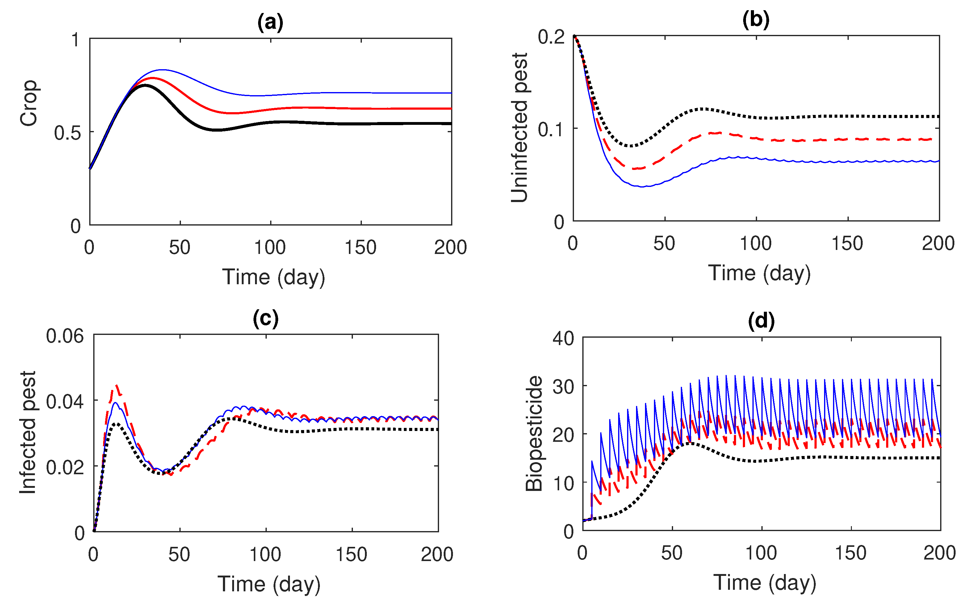
In Figure 1, the impulsive time interval for microbial biological pesticide release is 5 days, and releasing of biopesticide was considered in different rates: $v_i=0$ (i.e., without pesticides), $v_i=6$, and $v_i=12$. It is revealed that susceptible pest population decreases with an increase in the release rate of biopesticides.

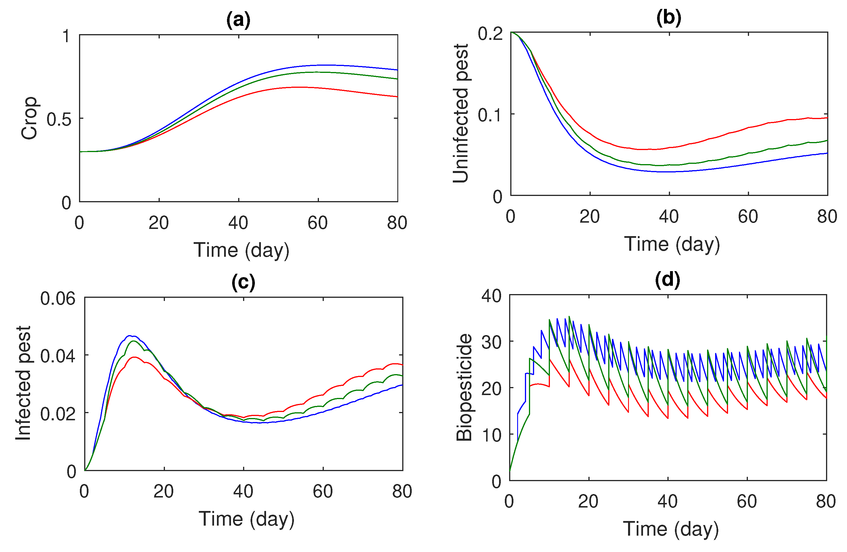
In Figure 2, by taking different impulsive intervals, biopesticide is applied to the system. A better result is obtained for lower intervals (2 days) but, with a higher release of biopesticide, pests are present in the system. From Figure 1 and Figure 2, we can conclude that pest control using only biopesticides is very costly and a time-consuming process.

Recall that in our model we take ${\tau }_1$ as the time period for biopesticide spraying (generally a virus particle) and ${\tau }_2$ as the time period for chemical pesticide sprays. In Figure 3 we see the effect for the same time intervals, ${\tau }_1={\tau }_2=5$ days, whereas in Figure 4 we see the effect for different time intervals, ${\tau }_1=3$ days and ${\tau }_2=2$ days.

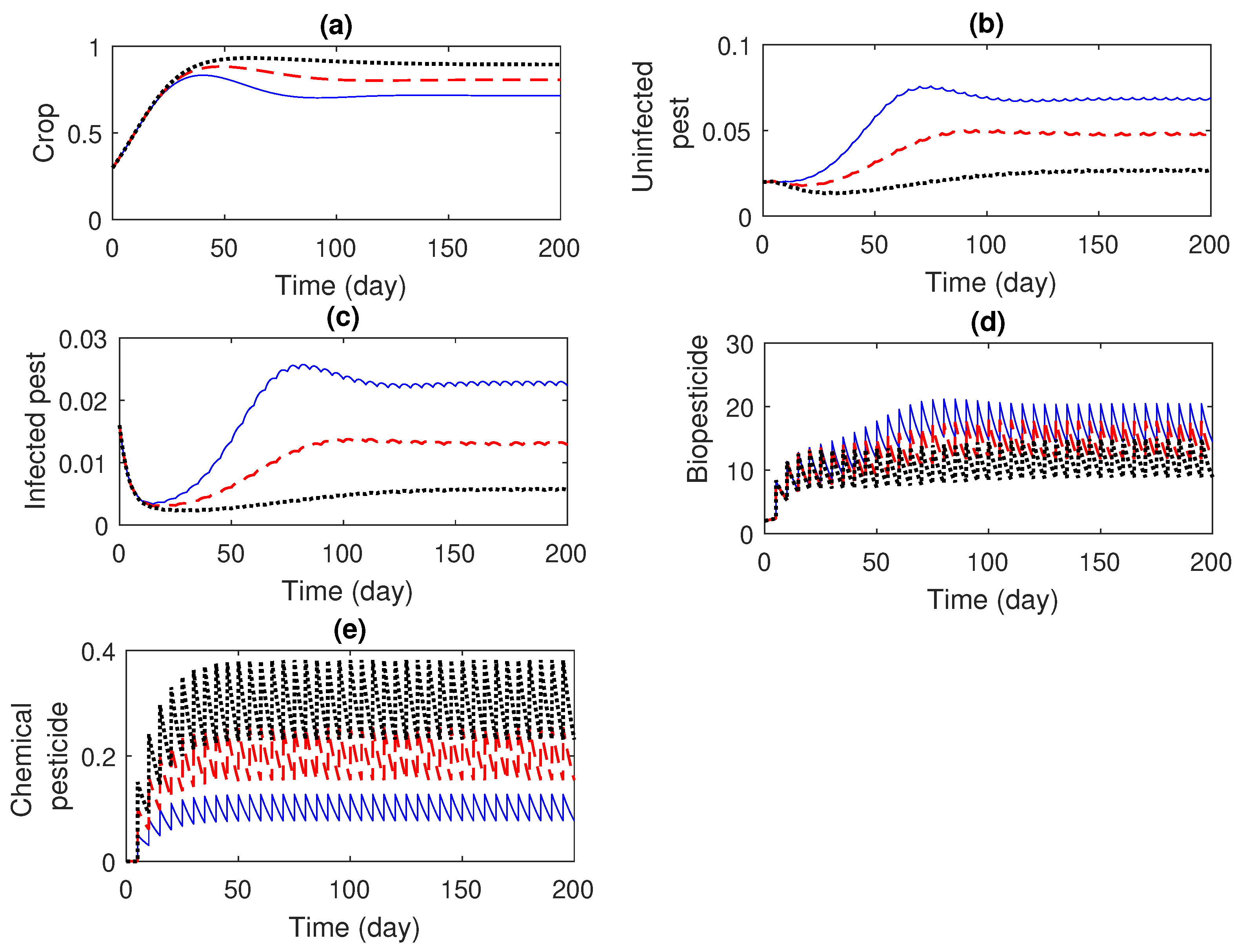
If both microbial biopesticides and chemical pesticides are released simultaneously, with an equal time interval of 5 days, then the extinction of both infected and susceptible pest populations is possible (see Figure 3).

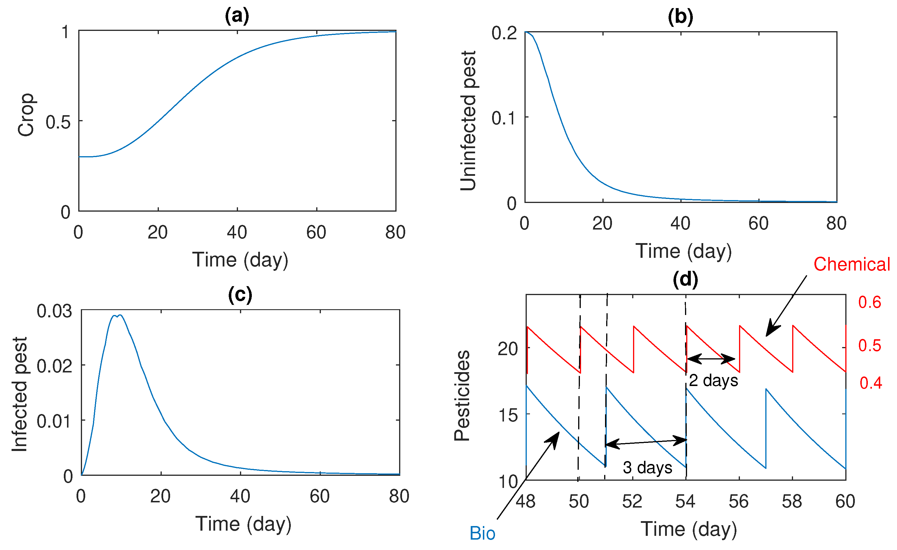
Figure 4 illustrates the dynamics of the double impulse with different impulse intervals. Double impulses occur at the time which is the common multiple of the two intervals. For example, if we take ${\tau }_1=2$ and ${\tau }_2=3$, then simultaneous impulses will occur at the times $t=6$, $t=12$, $t=18$, and so on. Figure 4 is the most important figure characterizing the impact of two different but simultaneous impulses on the total pest population with different time intervals. It is observed that for $v_i=12$, $s_i=0.15$, ${\tau }_1=3$, and ${\tau }_2=2$, the total pest population becomes extinct. In Figure 4d, the impact of double impulses occurs at $t=48$, $t=54$, $t=60$ days, etc., which are common multiples of the two intervals ${\tau }_1=2$ and ${\tau }_2=3$.

It is also numerically checked that when the rate of the impulse control is high, a comparatively lower interval can be taken for cost-effectiveness of the process.

Thus, the advantage of the impulsive control is that we can determine the proper rate and a suitable interval of giving controlling agents in the system.

5. Discussion and Conclusions

In the present research, we studied impulsive periodic applications of integrated pesticides, that is, simultaneous use of biopesticide and chemical pesticide in a pest management system. We proposed a two-impulse mathematical model using an impulsive differential equation to observe the impact of periodic application of the combined pesticides in impulsive modes.

In the previous models available in the literature, chemical and biological pesticides were used in the model in a continuous way. In contrast, here, we used them in an impulsive periodic way. Consequently, a two-impulse mathematical model was established. Moreover, in the proposed model, we took chemical pesticides concentration as the model population, which is a novel approach.

Stability theory (Floquet theory) and numerical calculations were used to examine the system dynamical behavior. We determined the conditions under which the impulsive system will be stable both locally and globally. For example, the local stability of a pest-free periodic orbit was established. The dynamics varied with the rate of both biopesticide recruitment and the chemical pesticide concentration.

Chemical pesticides minimize the oscillations in the system and make the system stable in a shorter time. Numerical and analytical analysis reveals that increasing frequency of pesticide application will require less administration of biopesticide and chemical pesticide, which is economically beneficial and environmentally safe.

Our research is directed to optimize and find the right combination of pesticides with maximum benefit to the crop plant. The numerical simulation also shows that control over the spraying of chemical pesticides is needed to control pests and minimize the cost of cultivation. On the other hand, chemical pesticides may have negative environmental implications due to their lingering effects; nonetheless, the best control approach provides the least amount of collateral damage to the environment.

In a nutshell, the promising feature of the system is the combined use of the pesticides in impulsive control methods that reduce the cost and negative effects on the environment. Using a combination of pesticides to deliver the pesticide can save the cost and reduce the side effects of chemical pesticides. Our obtained results will give a new perspective to farmers who implement this in a real-world setting.

In the future, one can extend this work to an optimal impulsive system for cost-effectiveness of the control process.

References

- Al Basir, F.; Banerjee, A.; Ray, S. Role of farming awareness in crop pest management—A mathematical model. J. Theor. Biol. 2019, 461, 59–67. [Google Scholar] [CrossRef]
- Ndolo, D.; Njuguna, E.; Adetunji, C.O.; Harbor, C.; Rowe, A.; Den Breeyen, A.; Sangeetha, J.; Singh, G.; Szewczyk, B.; Anjorin, T.S.; et al. Research and development of biopesticides: Challenges and prospects. Outlooks Pest Manag. 2019, 6, 267–276. [Google Scholar] [CrossRef]
- Chattopadhyay, P.; Banerjee, G.; Mukherjee, S. Recent trends of modern bacterial insecticides for pest control practice in integrated crop management system. 3 Biotech 2017, 7, 60. [Google Scholar] [CrossRef]
- Perring, T.M.; Gruenhagen, N.M.; Farrar, C.A. Management of plant viral diseases through chemical control of insect vectors. Annu. Rev. Entomol. 1999, 44, 457–481. [Google Scholar] [CrossRef] [PubMed]
- Ghosh, S.; Bhattacharya, D.K. Optimization in microbial pest control: An integrated approach. Appl. Math. Model. 2010, 34, 1382–1395. [Google Scholar] [CrossRef]
- Bhattacharyya, S.; Bhattacharya, D.K. Pest control through viral disease: Mathematical modeling and analysis. J. Theor. Biol. 2006, 238, 177–197. [Google Scholar] [CrossRef] [PubMed]
- Fest, C.; Schmidt, K. The Chemistry of Organophosphorus Pesticides; Springer: New York, NY, USA, 1973. [Google Scholar] [CrossRef]
- Lenteren, J.C.V. Integrated pest management in protected crops. In Integrated Pest Management; Dent, D., Ed.; Chapman and Hall: London, UK, 1995; pp. 311–320. Available online: https://cir.nii.ac.jp/crid/1573950400276916864 (accessed on 20 January 2023).
- Flint, M.L. Integrated Pest Management for Walnuts; University of California Statewide Integrated Pest Management Project; Division of Agriculture and Natural Resources, University of California: Davis, CA, USA, 1987; Volume 3270, p. 3641. [Google Scholar]
- Stern, V.M. The bioeconomics of pest control. Iowa State J. Res. 1975, 49, 467–472. Available online: https://core.ac.uk/download/pdf/224978255.pdf (accessed on 20 January 2023).
- Liu, B.; Teng, Z.; Chen, L. Analysis of a predator-prey model with Holling II functional response concerning impulsive control strategy. J. Comput. Appl. Math. 2006, 193, 347–362. [Google Scholar] [CrossRef]
- Páez Chávez, J.; Jungmann, D.; Siegmund, S. Modeling and analysis of integrated pest control strategies via impulsive differential equations. Int. J. Differ. Equ. 2017, 2017, 1820607. [Google Scholar] [CrossRef]
- Wang, L.; Chen, L.; Nieto, J.J. The dynamics of an epidemic model for pest control with impulsive effect. Nonlinear Anal. Real World Appl. 2010, 11, 1374–1386. [Google Scholar] [CrossRef]
- Al Basir, F.; Noor, M.H. A Model for Pest Control using Integrated Approach: Impact of latent and gestation Delays. Nonlinear Dyn. 2022, 108, 1805–1820. [Google Scholar] [CrossRef]
- Abraha, T.; Al Basir, F.; Obsu, L.L.; Torres, D.F.M. Pest control using farming awareness: Impact of time delays and optimal use of biopesticides. Chaos Solitons Fractals 2021, 146, 110869. [Google Scholar] [CrossRef]
- Chowdhury, J.; Basir, F.A.; Takeuchi, Y.; Ghosh, M.; Roy, P.K. A mathematical model for pest management in Jatropha curcas with integrated pesticides—An optimal control approach. Ecol. Complex. 2019, 37, 24–31. [Google Scholar] [CrossRef]
- Tang, S.; Chen, L. Modelling and analysis of integrated pest management strategy. Discret. Contin. Dyn. Syst. Ser. B 2004, 4, 759–768. [Google Scholar] [CrossRef]
- Paez Chavez, J.; Jungmann, D.; Siegmund, S. A comparative study of integrated pest management strategies based on impulsive control. J. Biol. Dyn. 2018, 12, 318–341. [Google Scholar] [CrossRef] [PubMed]
- Kalra, P.; Kaur, M. Stability analysis of an eco-epidemiological SIN model with impulsive control strategy for integrated pest management considering stage-structure in predator. Int. J. Math. Model. Numer. Optim. 2022, 12, 43–68. [Google Scholar] [CrossRef]
- Liu, J.; Hu, J.; Yuen, P. Extinction and permanence of the predator-prey system with general functional response and impulsive control. Appl. Math. Model. 2020, 88, 55–67. [Google Scholar] [CrossRef]
- Tian, B.; Li, J.; Wu, X.; Zhang, Y. Dynamic behaviour of a predator-prey system with impulsive control strategy. Int. J. Dyn. Syst. Differ. Equ. 2022, 12, 493–509. [Google Scholar] [CrossRef]
- Kumari, V.; Chauhan, S.; Dhar, J. Controlling pest by integrated pest management: A dynamical approach. Int. J. Math. Eng. Manag. Sci. 2020, 5, 769–786. [Google Scholar] [CrossRef]
- Pang, Y.; Wang, S.; Liu, S. Dynamics analysis of stage-structured wild and sterile mosquito interaction impulsive model. J. Biol. Dyn. 2022, 16, 464–479. [Google Scholar] [CrossRef]
- Chowdhury, J.; Al Basir, F.; Cao, X.; Roy, P.K. Integrated pest management for Jatropha Carcus plant: An impulsive control approach. Math. Methods Appl. Sci. 2021, in press. [CrossRef]
- Tian, Y.; Tang, S.; Cheke, R.A. Dynamic complexity of a predator-prey model for IPM with nonlinear impulsive control incorporating a regulatory factor for predator releases. Math. Model. Anal. 2019, 24, 134–154. [Google Scholar] [CrossRef]
- Jose, S.A.; Ramachandran, R.; Cao, J.; Alzabut, J.; Niezabitowski, M.; Balas, V.E. Stability analysis and comparative study on different eco-epidemiological models: Stage structure for prey and predator concerning impulsive control. Optim. Control. Appl. Methods 2022, 43, 842–866. [Google Scholar] [CrossRef]
- Li, J.; Huang, Q.D.; Liu, B. A pest control model with birth pulse and residual and delay effects of pesticides. Adv. Differ. Equ. 2019, 2019, 117. [Google Scholar] [CrossRef]
- Liu, B.; Kang, B.-L.; Tao, F.-M.; Hu, G. Modelling the effects of pest control with development of pesticide resistance. Acta Math. Appl. Sin. Engl. Ser. 2021, 37, 109–125. [Google Scholar] [CrossRef]
- Alzabut, J. An Integrated Eco-Epidemiological Plant Pest Natural Enemy Differential Equation Model with Various Impulsive Strategies. 2022. Available online: http://earsiv.ostimteknik.edu.tr:8081/xmlui/handle/123456789/207 (accessed on 20 January 2023).
- Zhang, H.; Xu, W.; Chen, L. A impulsive infective transmission SI model for pest control. Math. Methods Appl. Sci. 2007, 30, 1169–1184. [Google Scholar] [CrossRef]
- Al Basir, F.; Chowdhury, J.; Das, S.; Ray, S. Combined impact of predatory insects and bio-pesticide over pest population: Impulsive model-based study. Energy Ecol. Environ. 2022, 7, 173–185. [Google Scholar] [CrossRef]
- Shi, R.; Jiang, X.; Chen, L. A predator-prey model with disease in the prey and two impulses for integrated pest management. Appl. Math. Model. 2009, 33, 2248–2256. [Google Scholar] [CrossRef]
- Klausmeier, C.A. Floquet theory: A useful tool for understanding nonequilibrium dynamics. Theor. Ecol. 2008, 1, 153–161. [Google Scholar] [CrossRef]
Figure 1.
Impact of biopesticide application in impulsive mode on system (1). Evolution of (a) crop; (b) uninfected pest; (c) infected pest; (d) biopesticide. The set of parameters are , , , , , , , , , , , , , and . Here, the time interval is days and the rates of biopesticide release are (black line), (red line), and (blue line).
Figure 2.
Impact of biopesticide on system (1) for different impulse intervals and rates. Evolution of (a) crop; (b) uninfected pest; (c) infected pest; (d) biopesticide. Red line indicates and , green line indicates and , and blue line indicates and .
Figure 3.
Impact of both biopesticide and chemical pesticide on system (1) with the same impulse interval, . Evolution of (a) crop; (b) uninfected pest; (c) infected pest; (d) biopesticide; (e) chemical pesticide. The rates of impulses are and for black dotted color; and for red dashed line; and and for blue solid line.
Figure 4.
Impact of both biopesticide and chemical pesticide on system (1) with same impulse interval, , , and where the rates of impulses are and . Evolution of (a) crop; (b) uninfected pest; (c) infected pest; (d) pesticides (biopesticide in blue, chemical pesticide in red).
Disclaimer/Publisher’s Note: The statements, opinions and data contained in all publications are solely those of the individual author(s) and contributor(s) and not of MDPI and/or the editor(s). MDPI and/or the editor(s) disclaim responsibility for any injury to people or property resulting from any ideas, methods, instructions or products referred to in the content. |
© 2023 by the authors. Licensee MDPI, Basel, Switzerland. This article is an open access article distributed under the terms and conditions of the Creative Commons Attribution (CC BY) license (https://creativecommons.org/licenses/by/4.0/).
Share and Cite
MDPI and ACS Style
Al Basir, F.; Chowdhury, J.; Torres, D.F.M. Dynamics of a Double-Impulsive Control Model of Integrated Pest Management Using Perturbation Methods and Floquet Theory. Axioms 2023, 12, 391. https://doi.org/10.3390/axioms12040391
AMA Style
Al Basir F, Chowdhury J, Torres DFM. Dynamics of a Double-Impulsive Control Model of Integrated Pest Management Using Perturbation Methods and Floquet Theory. Axioms. 2023; 12(4):391. https://doi.org/10.3390/axioms12040391
Chicago/Turabian StyleAl Basir, Fahad, Jahangir Chowdhury, and Delfim F. M. Torres. 2023. "Dynamics of a Double-Impulsive Control Model of Integrated Pest Management Using Perturbation Methods and Floquet Theory" Axioms 12, no. 4: 391. https://doi.org/10.3390/axioms12040391
Note that from the first issue of 2016, this journal uses article numbers instead of page numbers. See further details here.