1. Introduction
Population density variations of interacting species in ecosystems are often modelled as discrete-time systems using difference equations (such as the Ricker model [
1]). Our study is motivated by the dynamical properties of discrete systems with an arbitrary step size. We consider a simple Ricker-type predator-prey system in discrete form, with a unit time step, given by
where
and
denote the prey and predator population at time
t, respectively;
r is the rate of prey population increase;
K is the prey carrying capacity,
is the predator attack rate;
is the conversion rate of eaten prey to sustenance for the predators; and
c is the predator starvation rate in the absence of prey [
2,
3]. The parameters
and
c are real and positive constants. The system (
1) is used to calculate the annual population densities after a time step of one year [
2]. We extend the Ricker-type model with arbitrary constant step size
h as
where
System (
2) is the generalised version of (
1) that considers the unit increments as a parameter such that system (
2) is the same as system (
1) if
.
In this paper, we also consider models such as Lotka-Volterra
where
h is the discrete step size. The step size
h plays a critical role by permitting the users to choose an appropriate time discretisation for each model. We observe that these generalized discrete systems incorporating an arbitrary fixed step size are forward Euler’s approximations of the respective continuous-time systems.
Beyond the step-size selections, the robustness of the model parameters is critical; however, it is often a source of uncertainty in models based on real data. A slight variation of the model parameters may change the equilibria and directly affect the system stability and robustness of solutions of the system [
4,
5,
6]. If the parameters are estimated from data, lack of information and the inability to collect sufficient real-world data in ecological systems can lead to an imprecise set of model parameters [
7]. Therefore, investigating a suitable set of parameters that agrees with the selection of stable or unstable dynamics is essential when constructing population models—especially in approximating continuous-time systems [
8] (see Acknowledgements for further clarification).
Following the idea of parametrising the step size, ref. [
9] derived the stability properties for a continuous-time Lotka-Volterra-type predator-prey system with scaled model parameters and showed unstable and stable population dynamics for derived conditions in step-size selections (see [
10,
11] for similar studies for Lotka-Volterra-type predator-prey models). To the best of our knowledge, no study has investigated the dynamic inconsistency under arbitrary step size for the Ricker-type ordinary differential equation (ODE) predator-prey model [
12], as given by
Hence, we study the required conditions for stable and unstable population dynamics of ODE system (
5) and their discretised system (
2) with generalised step size. Consequently, the results identify similar or different dynamical properties of approximated discrete systems compared to the corresponding continuous-time model.
We perform a comparable study on qualitative analysis of the stability properties of a commonly used continuous-time population model, a logistic growth Lotka-Volterra-type predator-prey system [
13]
Here, the prey population is influenced by the prey natural growth, prey restricted growth in terms of prey carrying capacity and prey death caused by predator attacks. The predator abundance is governed by population growth due to predation and natural death. We indicate that the generalised Lotka-Volterra model (
4) is the approximated discrete system of the continuous-time ODE model (
6).
The dynamical properties of predator-prey systems of continuous-time models have been studied extensively in the literature (see the examples at [
14,
15,
16]), but the factors that can perturb the dynamical properties (e.g., stabilising or destabilising the system) have not been fully analysed for discrete approximations of continuous-time systems.
We fill the gap of identifying the constraints that deliver similar or different dynamical properties of two continuous-time models and their approximated discrete system in terms of the arbitrary step size under parameter space. More precisely, we derive the stability properties of discrete systems associated with corresponding continuous-time models such that the interconnection of these two systems is purely observable.
The comparison of both approximated (discrete) and actual (continuous) systems reveals the conditions that must be satisfied by the time discretisation. Our study also highlights the importance of the changes in (some) model parameters that direct the system to have stable or unstable population dynamics. Therefore, our work contributes to choosing the best-suited step size for a particular discrete-time system and helps to understand the stabilising and destabilising factors of the continuous system and approximated discretised system under parameter space.
This paper is organised as follows. In
Section 2, a qualitative study to construct stability constraints is performed through a Jacobian analysis of the discrete systems followed by that of the continuous systems. In
Section 3, we derive the dynamical properties of discrete systems connected to the continuous-time systems and investigate the conditions that lead the system solutions to become stable in terms of selecting suitable sets of model parameters and determining the effects of the step size in time discretisation. We then demonstrate population dynamics to justify our theoretical findings through numerical simulations in
Section 4.
2. Equilibrium Stability and Dynamics
To understand the interconnection of dynamical properties in generic discretised systems with continuous-time systems under an arbitrary step size, we investigate the equilibrium points and the possible stable states of all Ricker-type and Lotka-Volterra systems mentioned in this paper. We first examine the system dynamics at the fixed points of the generalised discrete systems (
2) and (
4).
In order to develop stability conditions for discrete systems, we first consider the fixed point iteration formulation of a nonlinear map:
where
, and
F has a Lipschitz condition. A point
is said to be a fixed point satisfying
, where
F is a map, such that
, and
I is a region in
. It is proven that the fixed point
is asymptotically stable if there exists a norm such that
where
is the Jacobian matrix of the discrete system evaluated at
[
17]. Since we consider two dimensional systems, we have the following characterisations at
in terms of the two eigenvalues
and
of the Jacobian matrix of the iterated map:
- (i)
; a sink, locally asymptotically stable.
- (ii)
; a source.
- (iii)
One of and other ; a saddle.
- (iv)
One of and other ; non-hyperbolic.
Note that our investigation is based on this eigenvalue classification. Furthermore, we can find flip, saddle and Hopf bifurcations when we traverse the boundaries of different stability domains.
The equilibrium points for the Ricker-type and Lotka-Volterra discrete models can be obtained by solving
for
N and
P. For the generalised Ricker-type discrete model, (
9) implies
, and this also holds for the discrete Lotka-Volterra model, (
4). The fixed points of both the discrete formulations of the generalised Ricker-type discrete model and the discrete Lotka-Volterra model ((
2) and (
4), respectively) are the same, namely
,
and
. Further, these are the same equilibrium points obtained for the continuous time models since the same condition
was satisfied, and we use the same notation. We denote the Jacobians of discrete maps in (
2) and (
4) by
and
, respectively. Then, some analysis gives, after omitting the dependence on
t,
and
By using Jacobians, we derive the connection of the stability properties of the discrete systems to their respective ODE systems in the next section.
We then classify the equilibria of the continuous-time models (
5) (Ricker-type) and (
6) (Lotka-Volterra) based on the stability since unstable and stable equilibria behave differently in population dynamics. Both systems (
5) and (
6) have fixed points, namely
,
and
. Then, the Jacobian matrix of (
5) is
and the Jacobian matrix for (
6) is
We observe similar stability properties for both ODE models even though the Jacobian matrices are different. The Jacobian matrices evaluated at
are
Thus, the eigenvalues at
are
where
and
are the eigenvalues for system (
5) and (
6), respectively.
is unstable for both models regardless of any choices of parameter values since it is a saddle point such that one eigenvalue is positive and one is negative. This means that the population never returns to
after a small deviation of the population variation.
The Jacobian matrices evaluated at
are
and so
where
. The
value indicates a condition to determine the properties of the eigenvalues. Therefore, investigations for stability properties are presented in terms of
where appropriate. Then,
is asymptotically stable for both models if the parameters satisfy
(i.e.,
) since both eigenvalues are then real and negative. This means that, if there is a small deviation of the population densities away from
, the prey and predators can return to prey-carrying capacity (
) and no predators, respectively.
This implies that the prey population can be sustained by reaching its maximum carrying capacity without the presence of predators even if there are a small number of predators present in the ecosystem or if the prey population experiences high mortality. Moreover, this case shows the predator-prey existence under low predator populations where their ability to survive through food availability is determined by . On the other hand, for both models, is an unstable saddle point if and if is a non-hyperbolic point where the system dynamics depend on the nonlinear terms of the model equations since it cannot be predicted from the eigenvalue analysis of the Jacobian matrix.
The Jacobian matrices evaluated at
are
and since these Jacobian matrices are the same for both ODE models, we obtain identical results for stability analysis. The eigenvalues calculated for
satisfy the characteristic polynomial
where
and
. Thus,
where
,
. Note that, if
, the imaginary component for the continuous-time models is
, and the larger the imaginary component is, the more oscillatory are the dynamics (note that the maximum imaginary component occurs when
). The system stability status at a particular equilibrium point can be observed by looking at the sign of the eigenvalues and whether they are real or complex. We can conclude that
is asymptotically stable if
with oscillatory dynamics if
, and
is an unstable saddle point if
.
is the only non-trivial equilibrium point that has positive populations for both prey and predators. Note that, if
, we can have a non-hyperbolic property.
3. Deriving Connections of Dynamical Properties in Discrete and Continuous Systems
The connections between discrete systems and ODE systems are derived under arbitrary step size. Stability analysis for the discrete-time systems is simplified using derivations from the respective ODE systems where necessary. These stability constraints are observed through a Jacobian analysis, and the factors that could affect the system dynamics are analysed through variations of model parameters and by defining a particular range of step size.
Hence,
and
, where the eigenvalues of
and
are given in (
10), (
11) and (
13). Thus, from the eigenvalue analysis, we have locally asymptotic stability for discrete mappings if
and similarly for
. In the case that
, this leads to
and
. Therefore, depending on the step size and the eigenvalues of the continuous-time system, new conditions exist in discretised systems for stable population dynamics.
From the eigenvalue classification, is not asymptotically stable, but there is a saddle point if or for Ricker-type and Lotka-Volterra discrete maps, respectively. For , is asymptotically stable for the Ricker-type discrete model, if , and for the discrete Lotka-Volterra model, if . Furthermore, if and , is non-hyperbolic for both models. For , is a saddle point for the Ricker-type discrete model if one of the following conditions holds
- (i)
- (ii)
.
For , is a saddle point for the Lotka-Volterra discrete model if one of the following conditions holds
- (i)
- (ii)
In the case of the fixed point
, we can classify the stability associated with the two cases if the eigenvalues of
and
are given as
and
. From (
12), the eigenvalues satisfy
, where
and
. For
,
- (i)
If
and
are real and negative where
, then
is asymptotically stable if
This happens only if .
- (ii)
If both
and
are real and negative where
, then
is asymptotically stable if the step size satisfies
This happens if .
- (iii)
If both
and
are complex conjugate eigenvalues (say
), then, from the above,
and
. This occurs when
. With these complex eigenvalues, the population dynamics lead to oscillations with time. Then, the bound for the step size is
This can only happen if . Note that, if , then both eigenvalues have magnitude one.
For , say and , then is non-hyperbolic if . For , is non-hyperbolic if .
Overall, the stability constraints are different in continuous-time models and their corresponding discrete systems. A summary of the stability analysis of all eigenvalues for the Ricker-type and Lotka-Volterra discrete and continuous-time models are given in
Table 1. Stability criteria evaluated at equilibrium point
are similar for both Lotka-Volterra and Ricker-type models. At equilibrium point
, the stability conditions are similar for both models under continuous-time setting only and different otherwise. We consider the case (iii) when
for further simulations since it is a stable spiral where the population returns to a steady state,
.
Thus, additional constraints are required for stable population dynamics in approximated discrete systems compared with those in the continuous-time system (which is
). Therefore, the model dynamics of approximated discrete systems depend on the selected step size and (some) model parameters. We use (
15) to observe the stability with different step sizes and ranges of model parameters in the next section.
4. Numerical Results
We present a numerical simulation study for the Lotka-Volterra and Ricker-type discrete systems to illustrate the theoretical findings discussed in
Section 3. The stability condition (
15), where the discrete systems become stable at
, are demonstrated for some parameter ranges and step sizes. The impacts of model parameter variations on the system that change the model dynamics are then investigated through a few examples. This numerical study clearly demonstrates the changes to the population over time in the long-term scale.
We observed that some parameters impact the system dynamics and can stabilise or destabilise the populations if the time discretisation is fixed. In our discrete-time models, model stability is governed by the parameters
and
r according to the derivation of (
15) given that step size
h is fixed. We first observed the stability condition (
15) for discrete systems at unit step size
by assigning the parameter values described in [
2], where
and
. Then,
and
(note that we use these parameters for the numerical simulation study of this paper; some model parameters are subject to change depending on the analysis, and changes to the model parameters are given in each figure caption). Then, (
15) specifies stability for step size
where
and
In this case, since the eigenvalues are complex, the size of the imaginary component of the eigenvalue evaluated at equilibrium point
is
. For this choice of parameters with step size
, the system is not asymptotically stable at
since annual discretisation does not satisfy
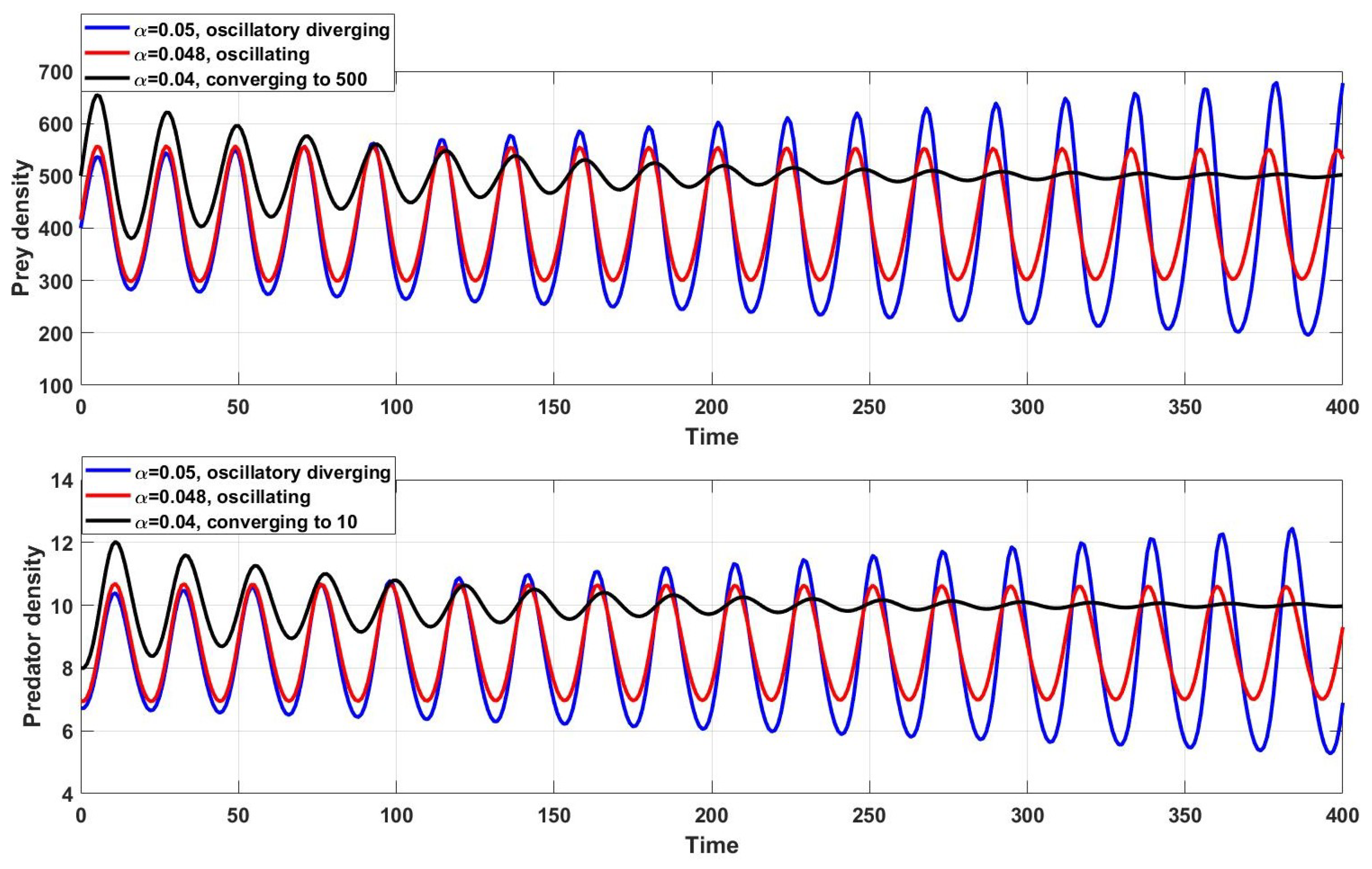
. Thus, the system dynamics diverge while oscillating around the equilibrium point
(blue curves in
Figure 1). If
with the other parameters the same and a one-year step size
, then the system may not become asymptotically stable since
and
.
In this case, the condition for stability in Equation (
15) is violated:
. The populations seem to be converging to
but oscillates around
(red curves in
Figure 1). If
and
with the other parameters the same, then
and
; thus,
, and the condition (
15) is true for this case. Therefore, the populations converge to
; see the black curves in
Figure 1. Thus, there is considerable sensitivity to the choice of parameters and, hence, to the step size, which controls the dynamics of the model.
Moreover, if we choose
, rather than
as previously, where
is a small positive value and the other parameters are as in [
2], then
and so (
15) gives
Then, for the step size
, the condition (
15) is true such that the system generates populations that converge to the fixed points (except for
). Therefore, if the step size is fixed, a small deviation of a model parameter or specific parameters that define model stability can make dramatic changes in the population dynamics.
Returning to the case of
, we varied
c by
for the step size
where
is a small positive constant value. The numerical results of population densities over time in
Figure 2 confirm the stability conditions developed for discrete models as in Equation (
15). For small values of
near zero, the populations are oscillatory diverging; see the blue curves in
Figure 2. Special dynamics are observed for
(red curves in
Figure 2), in which case,
and corresponds to the case of
studied previously.
Fixed point convergence is observed for
, which satisfies the stability condition in (
15); see the black curves in
Figure 2. The population dynamics according to the small changes of the parameter
c shows how critical the sensitivity of the parameters is. This is valid for other parameters that affect the stability of the discrete model—in our case,
and
r. Moreover, the numerical simulations of the discrete models support the developed analytical results in discrete systems.
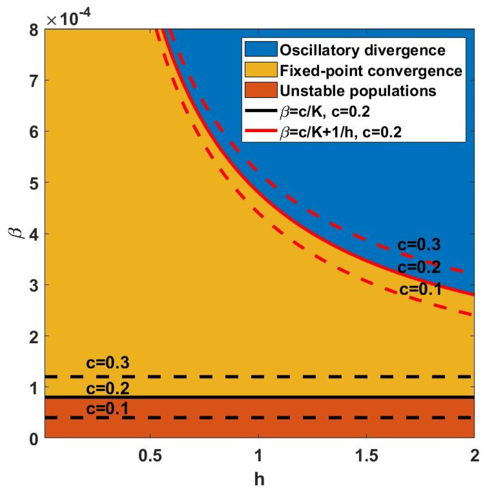
Figure 3 shows the fixed-point convergence region (yellow) for
, where
. Therefore, parameter
c has different boundaries for converging populations and preserving positive predator populations as demonstrated in the red and black curves of
Figure 3, respectively.
Special dynamics of system (1) are observed when
, which is on the upper bound of the fixed-point converging region (the red curves in
Figure 1). The black curves in
Figure 1 represent the converging predator and prey densities to their fixed points as the
is chosen from the yellow region of
Figure 3. If
is chosen from the oscillatory divergence region, the predator-prey densities tend to oscillate continuously and increase in amplitude; see the blue curves in
Figure 1.
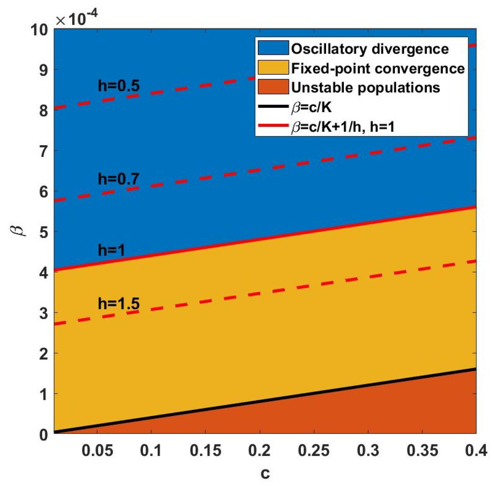
As a guide to selecting a suitable step size
h with the required stability property, the impacts of variable step sizes are investigated (see
Figure 4). The fixed-point convergence region becomes larger for small step sizes.
Figure 4 indicates that larger step sizes are more likely to show oscillatory divergence.
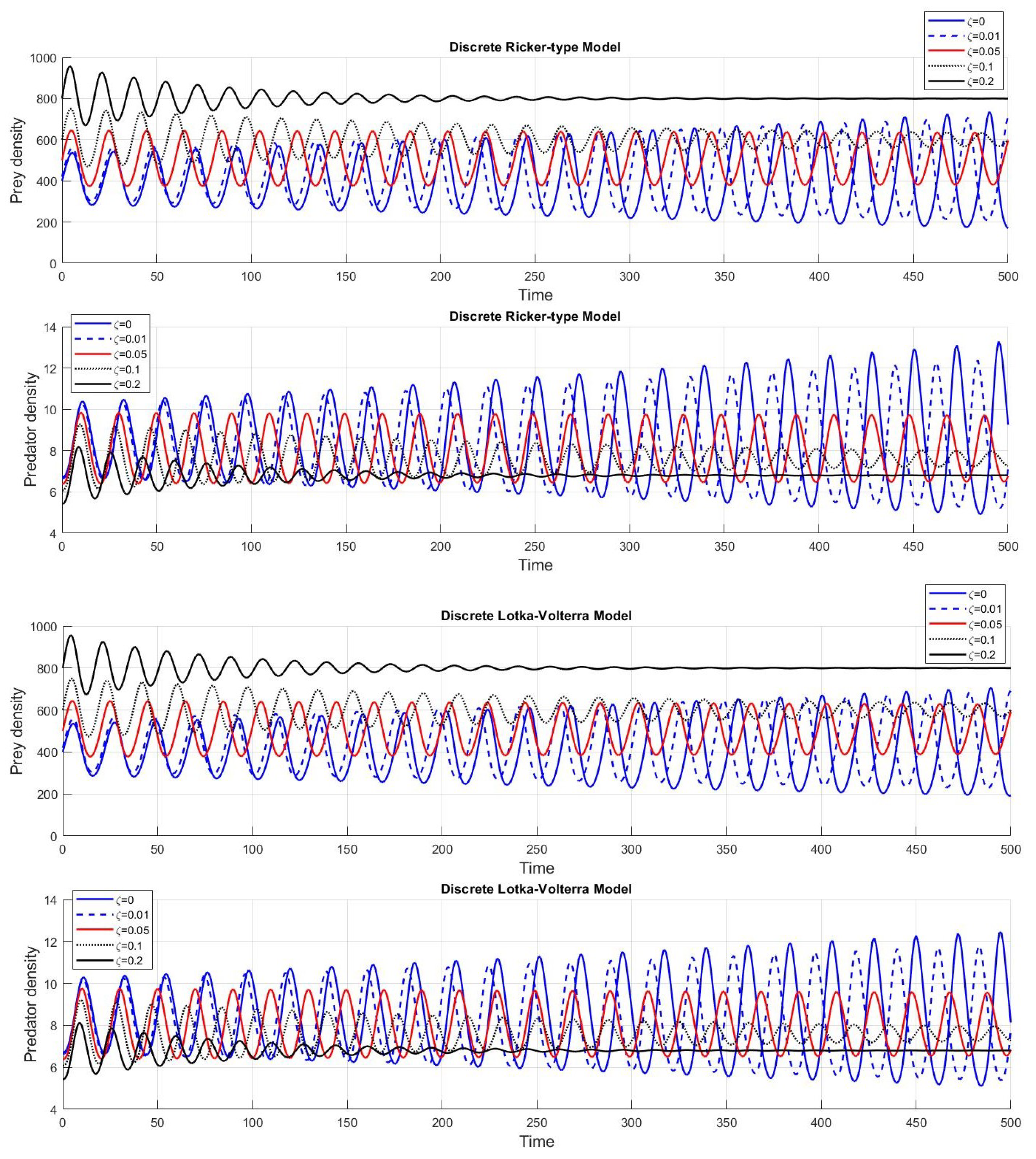
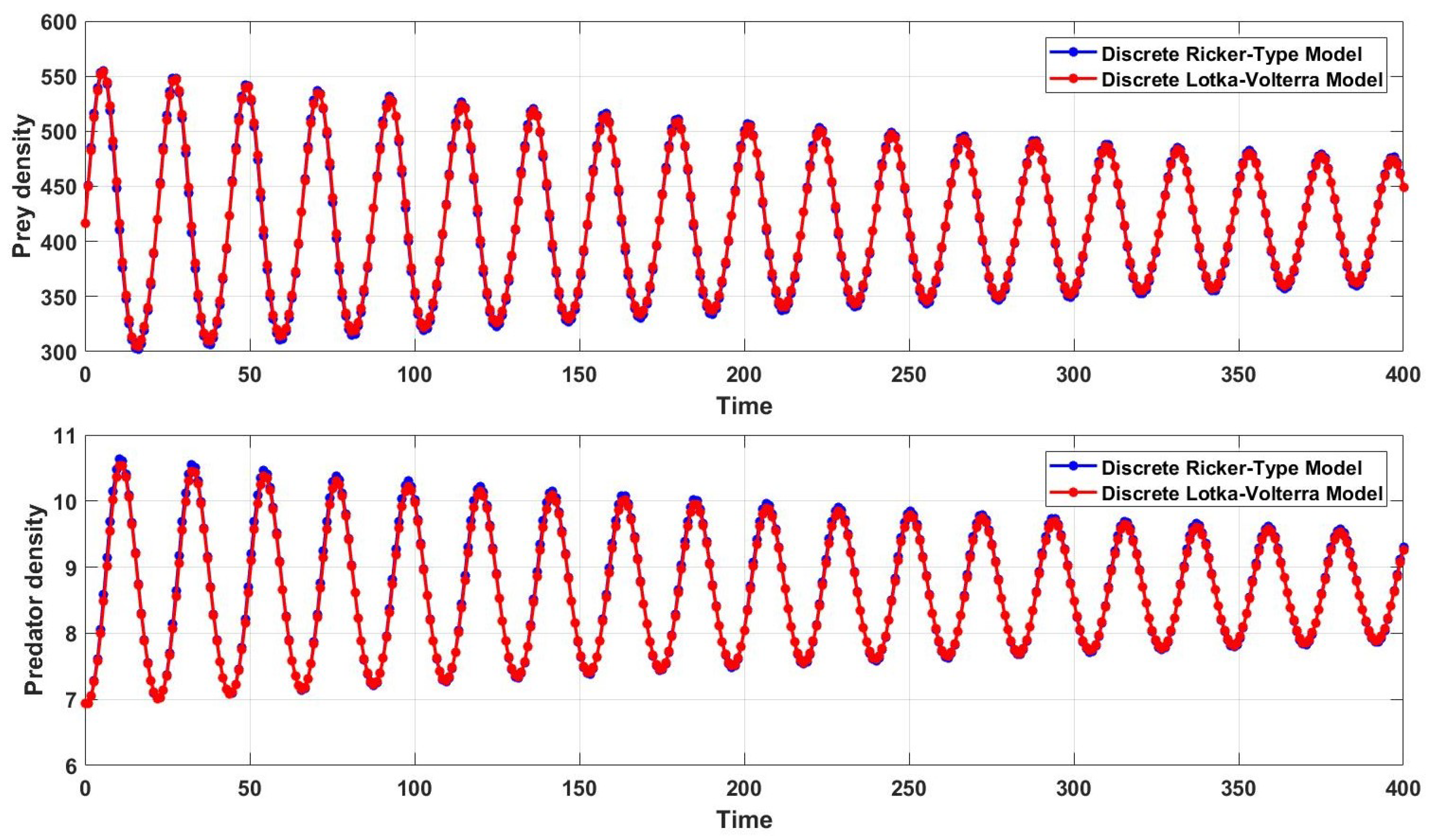
Even though the model structures of the discrete Ricker-type and Lotka-Volterra models are different, the derived stability conditions for these models are similar in certain cases. We examine the frequency plots of the population dynamics for both models with different step sizes. The red and blue curves in
Figure 5 provide evidence of the special behaviour when
(with
). These curves have a similar pattern that converges to a fixed point at a later time. The continuously converging pattern of these curves shows similar characteristics of the fixed-point convergence at the beginning, and, from the long-time observations, the populations never approach fixed points. Therefore, this is an exceptional case that behaves as an upper bound for the fixed-point convergence region.
5. Discussion and Conclusions
We investigated the stability of the population dynamics of Ricker-type and Lotka-Volterra discrete and continuous-time population models. Based on the Jacobian analysis, important constraints were generated to identify the stability regions of the discrete systems. The generalised discrete systems can be viewed as the Euler numerical scheme of the approximate solution of the continuous-time models.
The discretised solution may or may not have the same properties as observed in the original continuous-time model. Therefore, a qualitative analysis of the model dynamics in both the original continuous-time model and the relevant discretised system is essential when modelling to inform ecological decisions. We showed that the two models have similar conditions to stabilise the system depending on the constraints as shown in
Table 1. This novel work increases the understanding of the similar behaviours of two structurally different predator-prey models, in a nonlinear setting.
The derived stability properties for continuous-time and approximated discrete-time solutions are different at each equilibrium point. Therefore, choosing a suitable time discretisation depends on the stability criteria that are determined by the dynamical properties. Our results are outlined in
Table 1, which includes the results for asymptotic stability, non-hyperbolic stability and saddle points. We assume the populations in real ecosystems coexist at, or move to, a stable state, which is
with asymptotic stability. Therefore, selecting a suitable time discretisation is essential to approximate the respective continuous-time system if the model parameters are given.
We highlighted the significance of understanding the choices of model parameters that impact the stability of the system. Some parameters need to be verified carefully due to the strong effect on system dynamics, such as the parameters determined by . Small changes in these parameters lead to large deviations in the population count when the step size of the time discretisation is fixed (e.g., one year). A prior analysis on the impact of selecting a suitable time discretisation that is relevant to selected parameter sets is essential for better performance of the models. We also numerically showed that the small changes in parameter values and step sizes stabilise or destabilise the system and form different dynamics in population densities.
Our results on the Ricker-type discrete model are consistent with the stabilisation that was found in [
3]. However, the discrete model stability analysis that shows the significance of dynamical properties over the parameter space goes beyond previous studies on investigating the stabilising and destabilising factors defined in [
18,
19]. Populations become more stable and converge to the equilibrium point if the step size is small. This generates a time discretisation (into small time intervals) where the discrete systems behave more closely to the continuous systems.
Certainly, to preserve the characteristics in numerical simulations, this idea supports the small step size recommendation in Euler’s scheme, since it is a first-order method [
20]. These results lead to selecting suitable values for the step size in terms of preserving the required stability states when approximating discrete systems to respective continuous systems. On the other hand, if the step size is too small, then, on larger systems, the simulations may take a very long time to run, especially over large time intervals. We note that there are non-standard discretisation methods of nonlinear ODEs to preserve the dynamic consistency regardless of the selection of the step size [
21,
22].
This is not a complete study of the dynamics of discrete mapping. For example, from (
7), we note
. Hence, we can study the fixed points of
, and the ensuing dynamics would lead to period-two dynamics depending on the nature of the map
F. The two models will have different dynamics in this regard. The theories on limit cycles and bifurcation analysis [
23,
24,
25] were not considered; however, this can be seen through our numerical simulations. Of course, this can be generalised to period dynamics of any integer order and potentially lead to chaotic dynamics (of iterations of the logistic map). Moreover, parameter-identification methods can be applied to estimate parameters within a chaotic system [
26].
The demonstrated stability analysis can be applied to other forms of two-species continuous-time and discrete-time population models in returning more complex dynamical systems, such as controlling species, functional responses, time delay [
27,
28] and the Allee effect. Our work can be extended to study the dynamics of three or more species systems [
29] and to understand the stabilising and destabilising factors before obtaining the model outcomes.
Finally, this work has implications in uncertainty quantification. In this setting, populations of models (with the same structure but different parameter sets) are constructed based on these models satisfying a set of common outputs. If there is sensitivity of the dynamics to the parameters, as is the case here, then this can make the process of uncertainty quantification also sensitive.
In conclusion, the stability criteria for the continuous-time models depend only on the model parameters defined by ; however, when the continuous-time models are discretised through numerical approximations, the stability criteria depend on the step size along with (some) model parameters. Therefore, the dynamical properties of the original ODE systems are different from the respective discretised systems with the same parameter values unless a suitable step size is defined.
To obtain a better understanding of the model dynamics, the discretised systems should be thoroughly investigated under an eigenvalue analysis to identify suitable step sizes that agree with the model parameters. In real predator-prey systems, prior knowledge of the system behaviour enhances the understanding of the factors that stabilise or destabilise the populations over time. If the parameters are estimated from a data set, this type of theoretical study provides a detailed analysis for selecting a suitable numerical simulation method that discretises the time component with step size.

 ,
, 


