
A Compound Class of Inverse-Power Muth and Power Series Distributions

1
Departamento de Matemática, Facultad de Ingeniería, Universidad de Atacama, Copiapó 1530000, Chile
2
Departamento de Ciencias Matemáticas y Físicas, Facultad de Ingeniería, Universidad Católica de Temuco, Temuco 4780000, Chile
3
Departamento de Estatística, Universidade Federal do Rio Grande do Norte, Natal 59078-900, Brazil
*
Author to whom correspondence should be addressed.
Axioms 2023, 12(4), 383; https://doi.org/10.3390/axioms12040383
Submission received: 25 February 2023
/
Revised: 28 March 2023
/
Accepted: 30 March 2023
/
Published: 16 April 2023
(This article belongs to the Special Issue Probability, Statistics and Estimation)
Abstract
:This paper introduces the inverse-power Muth power series model, which is a composition of the inverse-power Muth and the class of power series distributions. The use of the Bell distribution in this context is emphasized for the first time in the literature. Probability density, survival and hazard functions are studied, as well as their moments. Using the stochastic representation of the model, the maximum-likelihood estimators are implemented by the use of the expectation-maximization algorithm, while standard errors are calculated using Oakes’ method. Monte Carlo simulation studies are conducted to show the performance of the maximum-likelihood estimators in finite samples. Two applications to real datasets are shown, where our proposal is compared with some models based on power series compositions.
MSC:
62E10; 62F101. Introduction
A brief literature review reveals several distributions related to the power series (PS) distribution models, as shown in [1], which add a parameter to the distribution to provide more flexibility to the proposed models compared to the baseline distribution. The number of parameters depends on the composition of the baseline model, considering the classes of distributions. Some of the most relevant PS distributions are: extended Weibull power series proposed by Silva et al. [2]; Gompertz power series (GPS) by Jafari and Tahmasebi [3]; Burr XII power series studied in Silva and Cordeiro [4]; inverse Weibull power series (IWPS) presented by Shafiei et al. [5]; exponential Pareto power series introduced by Elbatal et al. [6]; Janardan power series by [7]; compound power series with the negative multinomial model introduced by [8]; generalized Burr XII power series performed by Elbatal et al. [9]; Inverse Gamma Power Series (IGPS), of three-parameter by Rivera et al. [10]; three-parameter Inverse Lindley power series (ILPS) proposed by Shakhatreh et al. [11]; four-parameter exponentiated inverse Lomax power series proposed by Hassan et al. [12]; and five-parameter exponentiated power generalized Weibull power series proposed by Aldahlan et al. [13], among others.
In this vein, we propose to study the composition between the recently proposed Inverse-Power Muth (IPM) distribution, introduced by Chesneau and Agiwal [14], which has a positive basis with three parameters, and the class of PS distributions proposed by Noack [15]. This allows us to develop models with more flexibility to fit data and a non-monotone hazard function for different applications, such as cancer and mortality studies, which may not have a monotonic hazard rate function. Furthermore, we highlight for the first time the use of the Bell distribution in this context.
The IPM distribution emerges as a distribution whose hazard function is non-mono-tonic [14]. This distribution is obtained by calculating the inverse of the Power Muth distribution [16], which in turn comes from the distribution proposed by Muth [17]. Such a distribution, compared to other lifetime distributions, has a less heavy right tail and has enough flexibility to accommodate a large panel of lifetime datasets [14]. Singh et al. [18] indicated that the Muth distribution has been proposed previously by Teissier to model the frequency of mortality related to the aging process. Muth had used it for reliability analysis; however, the same authors believed that they could not have seen this article while working with the distribution at that time. In a brief bibliographic review of the current literature, the article by Muth [17] is taken as a reference when generating new families of distributions, such as those proposed by Abdullah et al. [19] and Almarashi et al. [20]; these articles study the truncated family generation and the T-X generator, respectively. For our research, we will continue with the distribution name of Muth.
A random variable (r.v.) T follows an IPM distribution [14] with parameters , and , if its probability density function (PDF) is given by
Its cumulative distribution function (CDF) is given by
and its survival function is
The non-central moment for the IPM [14] distribution, i.e., , exists for and is given by
where , when , and when . An important feature of the distribution is the quantile function (QF), which is given by
where denotes the Lambert function. For any complex t, the Lambert function is defined as the inverse of the function . An implementation in R software is available through the LambertW package (Goerg [21]).
The paper is organized as follows: Section 2 presents the proposed model based on the IPM and the power series (PS) models, infinite linear combination expressions, and further examination of the moments for the model. Section 3 discusses the estimation of parameters using the expectation-maximization (EM) algorithm (Dempster et al. [22]) and the estimation of their respective variances applying Oakes’ method [23]. The performance of estimators in finite populations is studied in Section 4. In Section 5, two applications of the IPM-PS model are considered in comparison with other models based also on PS or IPM distributions. Finally, Section 6 presents the main conclusions of this manuscript.
2. The Model
Suppose that in a certain context, the event of interest can be developed by M non-observable concurrent causes. For example, in the context of cancer, those causes are represented by carcinogenic cells. Suppose now that M follows a PS distribution with probability mass function (PMF) given by
where is called the power parameter and is the power series.
Table 1 shows some distributions that belong to the PS family and that will also be used for the development of this research. The Bell distribution has been used loosely in the literature. Table 1 presents the values of , , and the parameter space for the distributions that we will use here. It should be noted that is the Bell number. Additionally, please note that we are considering , which indicates that we are using the zero-truncated version of the Poisson (ZTP) [24] instead of the traditional Poisson model.
2.1. Model Construction
Let be a r.v. denoting the a-th time at which one of the M possible concurrent causes produces the event of interest, for . Given M, let be independent and identically distributed r.v.’s following the IPM (, , ) distributions. The IPM-PS is defined as the marginal distribution of . The motivation to introduce this distribution is related to a competing risk scenario, where M possible causes can produce the event of interest and it is enough for a single cause to fail for the event of interest to occur, a scheme similar to that used in parallel systems with the particularity that the number of components, M, is random. The CDF for the IPM-PS model can be calculated as
As the are conditionally independent, given M, and identically distributed, then we have
Thus, the survival function of the IPM-PS model is given by
and its corresponding density function is given by
The hazard rate function is
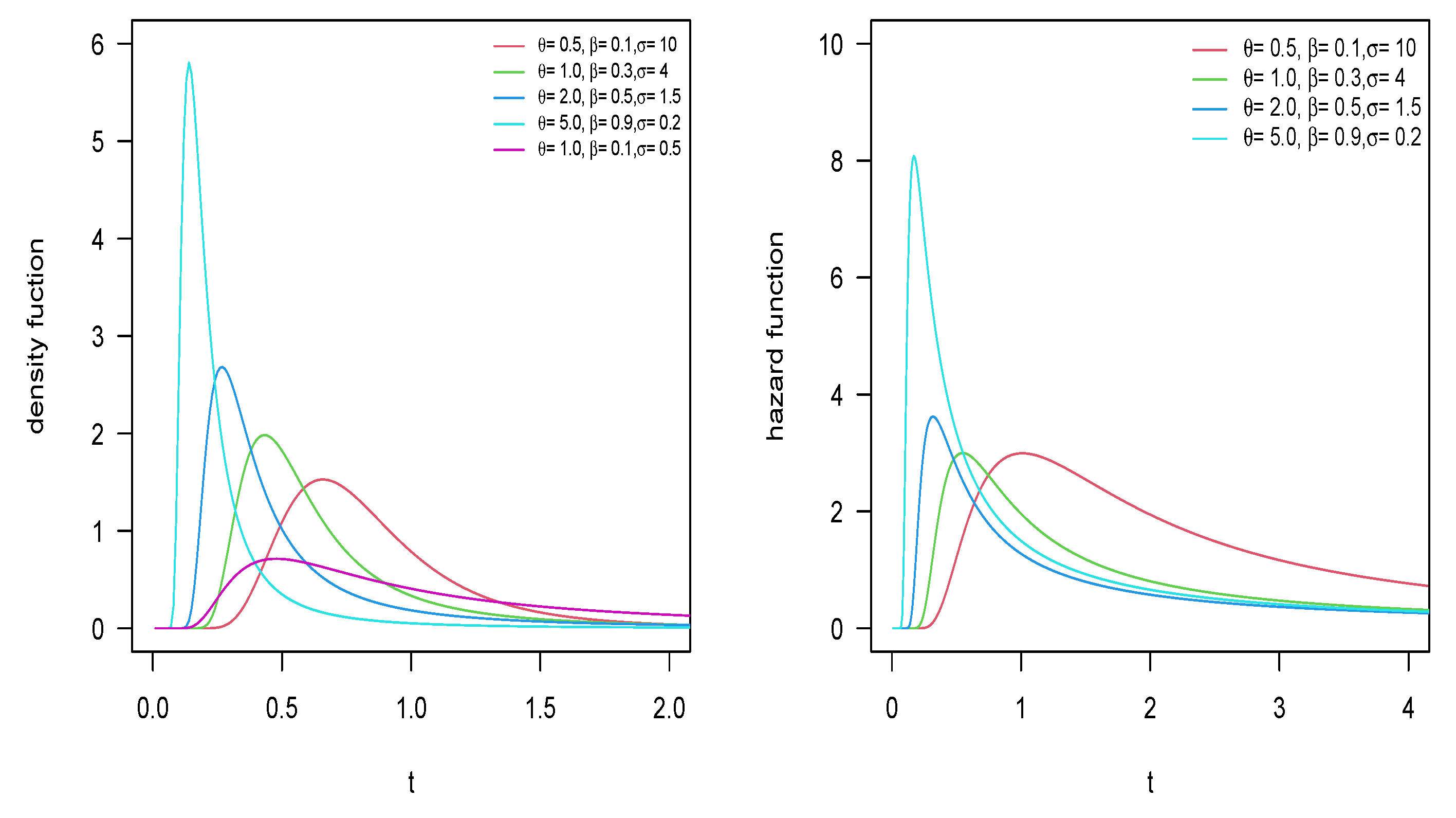
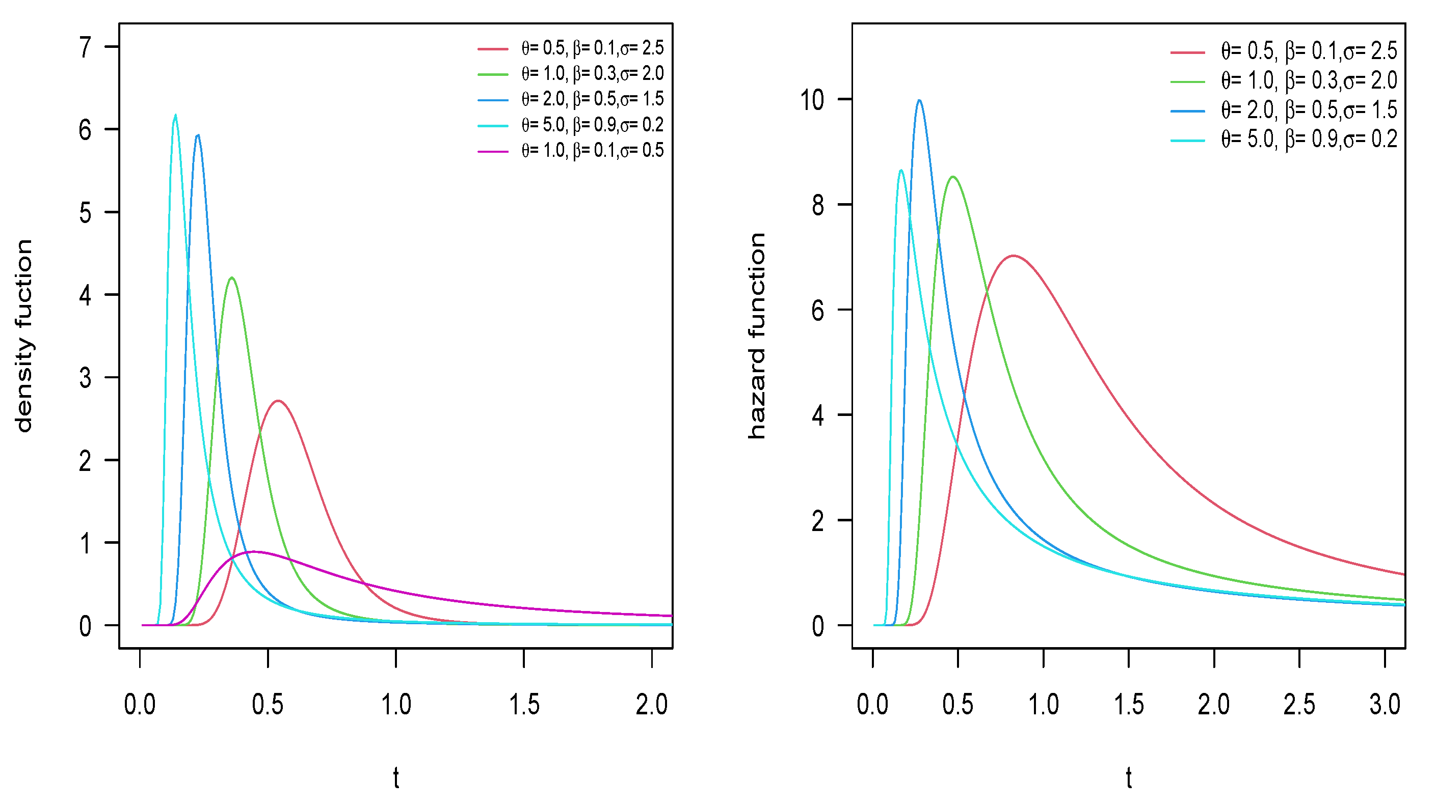
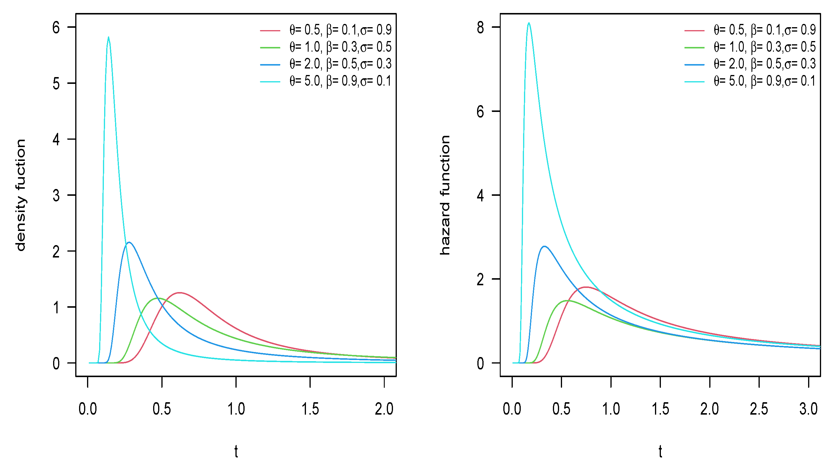
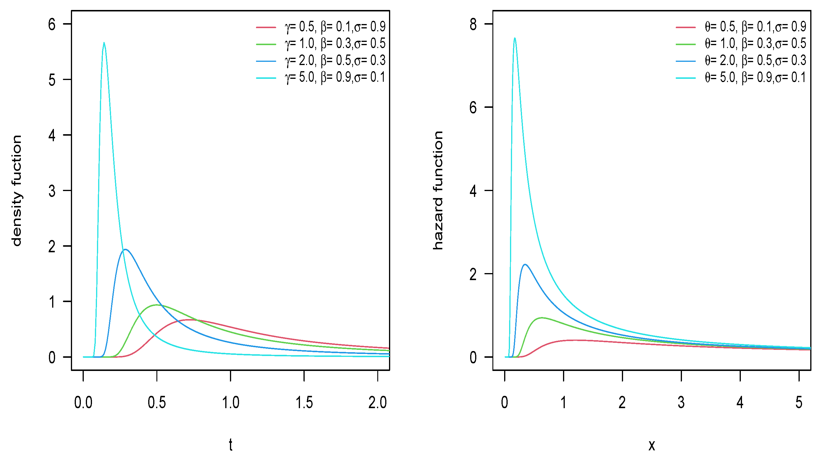
Figure 1 and Figure 2 present the PDF and hazard function of the Inverse-Power Muth Poisson (IPM-P) and Inverse-Power Muth Bell (IPM-B) models, where, for , , and , we can see that there are heavy tails on the right in their PDF, which suggests that the mean does not exist. In Appendix A, we present the same plots for the inverse-power Muth geometric (IPM-G) and inverse-power Muth logarithmic (IPM-L) distributions.
2.2. Model Properties
Proposition 1.
Let and considering the PDF for the IPM-PS given in Equation (4), it is determined that
where is the conditional PDF of T given the value M for the IPM distribution.
Proof.
Taking the derivative of Equation (2), we obtain
□
The PDF of the IPM-PS can be expressed as the infinite linear combination of IPM distributions, which will provide a wide use for the application of the EM algorithm, as will be shown in Section 3.
Proposition 2.
The r-th moment of the IPM-PS distribution, with , is given by
where is defined as
where for , and for .
Proof.
By definition of expected value, the r-th moment of the r.v. T is calculated as
By making the change, , and following Chesneau and Agiwall [14] in the given expression of moments, we have that
Therefore,
□
In the case that the moments tend to infinity. In Appendix B, we present explicit forms for for each of the PS cases considered.
From Table 2, we observed that the moments and variance are smaller as the parameters and take larger values.
2.3. Shannon Entropy
The Shannon entropy [25] measures the amount of uncertainty for a random variable. It is defined as . For the IPM-PS model, this measure is presented in the following proposition.
Proposition 3.
The Shannon entropy for the IPM-PS model is given by
where is the survival function of the IPM distribution, Muth and denotes the PDF of the Muth distribution.
Proof.
By definition, is given by
where is the PDF of the IPM distribution. Then, using the change of variable in the first integral of Equation (5), we obtain
On the other hand, by manipulating the second integral in (5), using the change of variable and considering the PDF of the Muth distribution, we obtain
then
Finally, using the change of variable in the third integral of Equation (5), we obtain
In Appendix C, we present explicit forms for the integral in Equation (9) for each of the considered cases of the PS.
2.4. Pseudo-Random Number Generator of the Model
To generate random numbers from the r.v. IPM-PS, we use the inverse transform method, which is summarized as follows (Algorithm 1).
| Algorithm 1 Simulating values of the IPM-PS model |
|
Where Q is the quantile function of the IPM model and is the inverse function of the power series, which can be seen in Appendix D.
3. Parameter Estimation
In the current section, we discuss the estimation of the parameters of the IPM-PS distribution, using the maximum-likelihood (ML) method. For a random sample of the IPM-PS model, the (observed) log-likelihood function for the parameter vector , is given by
The ML estimators are obtained by direct maximization of the log-likelihood function given in (10). As such a procedure requires a four-dimensional maximization problem, we propose an EM-type algorithm (Dempster et al. [22]) as an alternative and more robust process that allows the maximization of the likelihood function, considering some variables of the model as “latent” or unknown.
EM Algorithm
For this particular problem, the vector represents the latent variables, the vector denotes the observed data and the vector represents the complete data. Therefore, the complete log-likelihood function for the parameter vector , is given by
where
Let be the estimate of at the k-th iteration, and the function defined as the conditional expectation of . Given the observed data and the vector of parameters at the k-th iteration, it follows that
where
where . Following Gallardo et al. [26] and considering the function with the respective derivatives, the EM algorithm is summarized as following.
- E step: For , define and calculate:
- step M-I: is updated as the solution of the non-linear equationwhere is the sum of the elements of .
- step M-II: Given the vector , update by maximizingin relation to each of the parameters.
- If the convergence condition is reached, the algorithm stops. Otherwise, we return to step E for a new iteration.
Figure 3 shows the scheme for the EM algorithm for clarifying the way to use it.
By taking advantage of the complete log-likelihood function, the variance of the estimator of can be computed by Oakes’ method presented by Oakes [23]. This method computes the observed information matrix instead of the Fisher information matrix. Details of this method are provided in Appendix E. We highlight that in the literature, variance is usually obtained from numerical methods that approximate the observed information matrix associated with the log-likelihood function in relation to the parameters to be estimated. However, we highlight that the Oakes method provides an exact method for calculating this matrix, also avoiding possible approximation errors.
Asymptotic confidence intervals (ACIs) with confidence level , , can be constructed based on the asymptotic normality of the MLs, i.e.,
where .
4. Simulation Study
In this section, a simulation study is carried out to investigate the performance of the ML estimators for the IPM-PS model in finite samples. For this, the EM algorithm was used to calculate the estimates and their corresponding standard errors (SE) and the root of the mean squared error (RMSE). This process was replicated 1000 times with sample sizes of , and . For the parameters, the following were considered to be true values: in the IPM-P and IPM-B models and in the IPM-G and IPM-L models. For , and were considered to be true values; for ; and for in all the cases. The confidence level considered to build the ACIs is . The IPM-G, IPM-P, IPM-B, and IPM-L models were considered for this study.
From Table 3, Table 4, Table 5, and Table 6, as the sample size increases (, , and ), the bias of all the estimators decreases and the variances become smaller for each of the estimators. Standard deviations for all cases were also calculated, but are not reported here. These values were also close to the SE terms, which suggests that the variances of the estimators are well estimated. Finally, the CP terms converge to 0.95 as the sample size increases.
5. Applications
In this section, we present two applications of the IPM-PS distribution. The parameter estimation was performed based on the EM algorithm, as discussed in Section 3.
5.1. Application 1
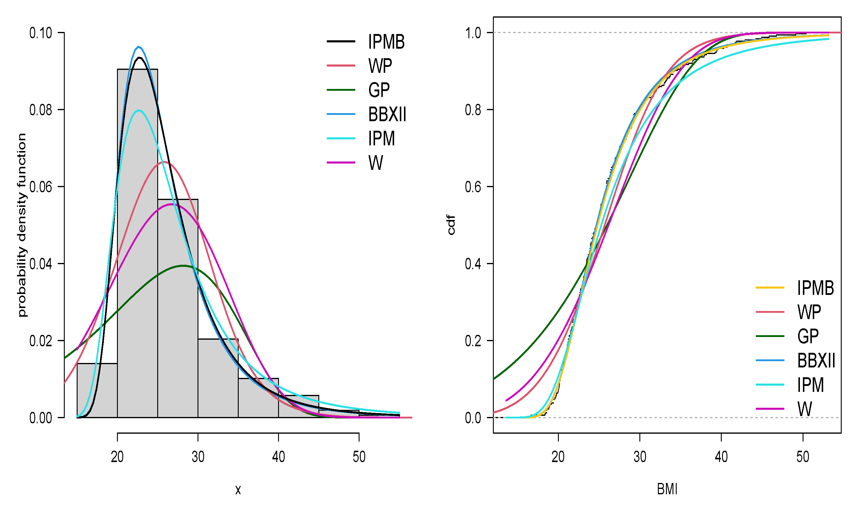
This dataset presents body mass index (BMI, weight/height) values and is available from the “bsamGP” package (Jo et al. [27]) of the “R” software [28], containing 314 observations. The BMI acts as an indicator to assess the nutritional status of the patients. For comparative purposes, the IPM-B, Gompertz–Poisson (GP), Beta Burr XII (BBXII), Weibull-Poisson (WP), IPM, and the Weibull (W) distributions were also considered.
Based on the Akaike information criterion (Akaike, [29]) and the Bayesian information criterion (Schwarz, [30]), we observe that the IPM-B provides the best fit to the dataset among the models considered, as confirmed in Table 7, where both the AIC and BIC criteria are the lowest values compared to the rest of the distributions. Furthermore, Figure 4 shows the corresponding fit of the different distributions that were compared.
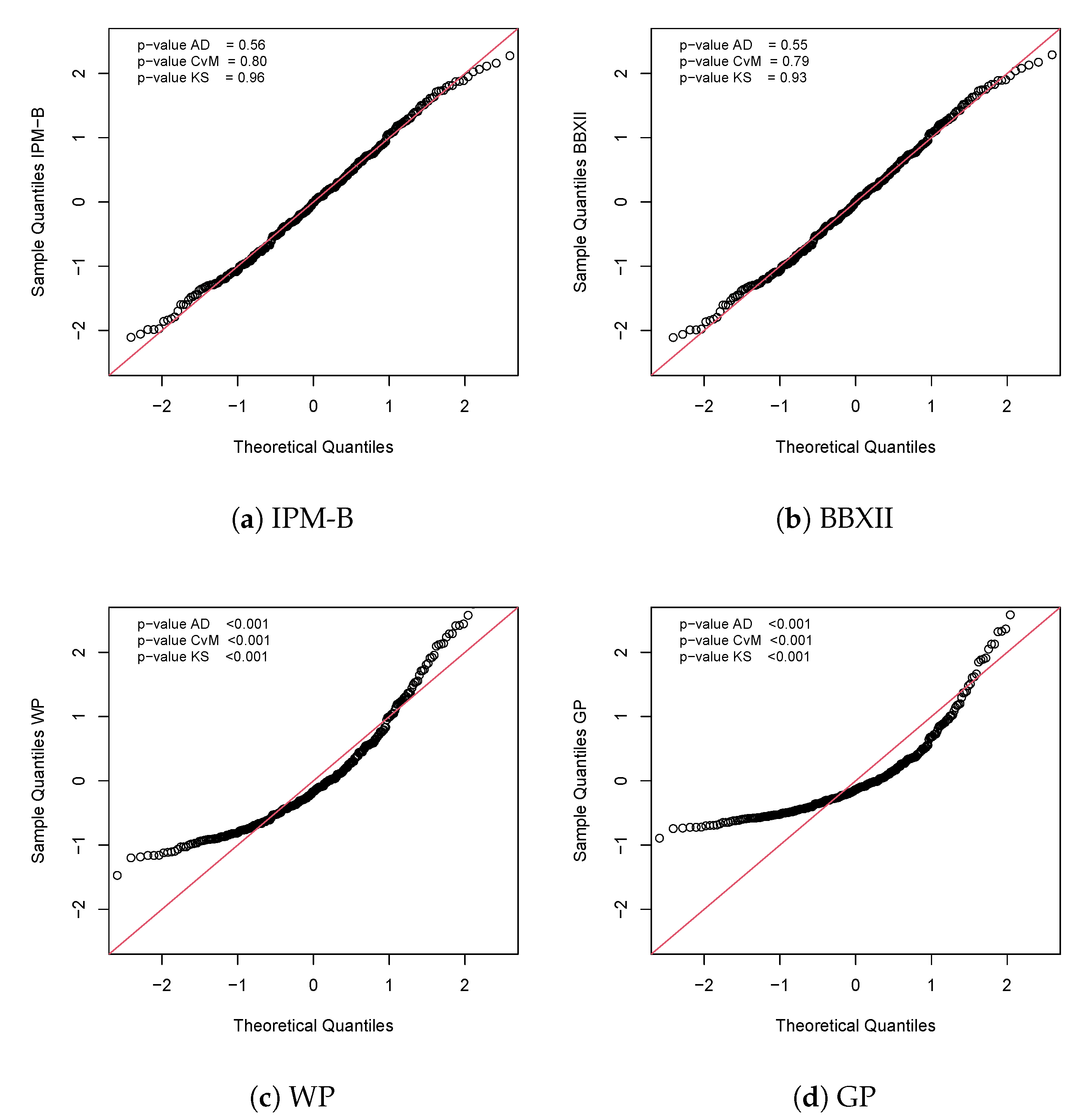
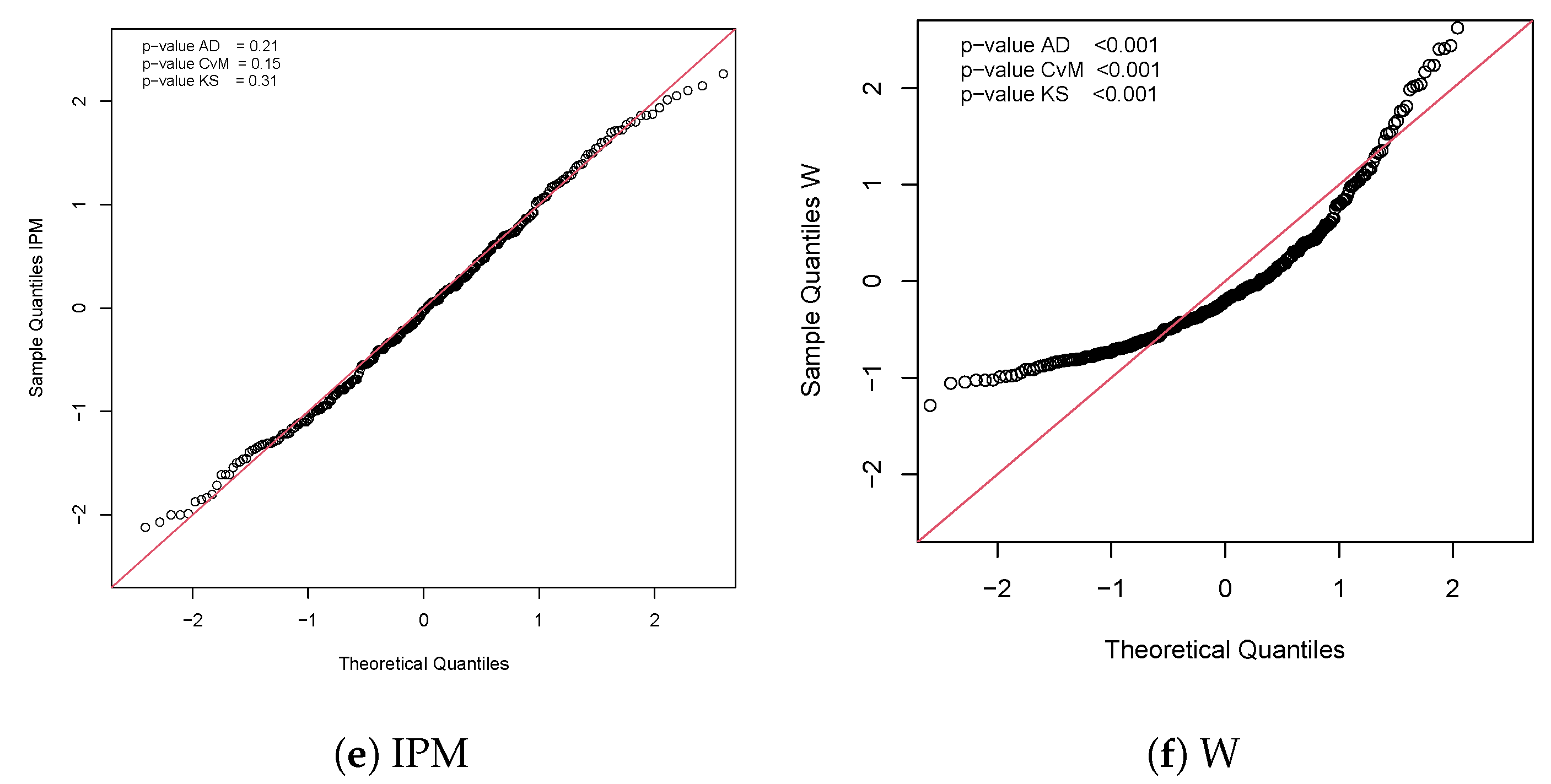
An alternative to check the adequacy of a model is to use the quantile residuals (QR, Dunn, and Smith [31]). If the model is appropriate, these residuals will have a standard normal distribution. Anderson Darling (AD), Cramer–von Mises (CvM), and Kolmogorov–Smirnov (KS) normality tests were performed to verify the normality of the QR. Figure 5 shows the QQ-plot for the QR in the IPM-B model and the p-values for the referred tests, suggesting that the residuals are normally distributed. Finally, Table 8 presents the point and interval estimates (based on the delta method) for the percentage of overweight patients, i.e., patients whose IBM is greater than 30 using the IPM-B, BBXII, IPM, and WP models. Please note that the IPM-B provides the more accurate 95% CI. At first, one might question whether 0.0002 is too small a difference. However, if we think about estimating the percentage of people who are overweight in a small country (say with 10 million inhabitants), this difference translates into a precision of 2000 people in the interval estimate.
5.2. Application 2
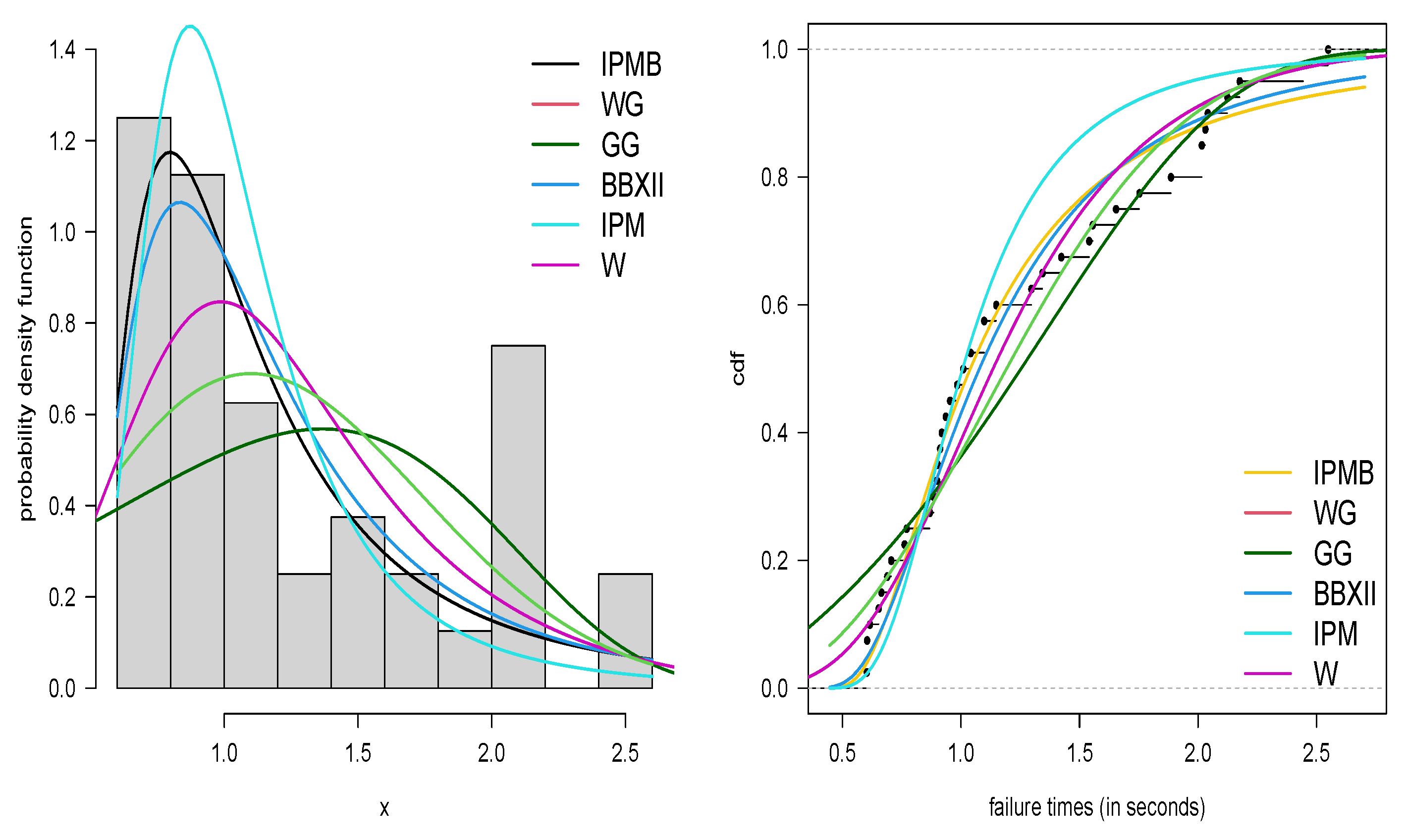
This dataset was taken from Murthy et al. [32], and is related to the failure times of 40 articles. For the current example, the IPM-P, Gompertz–Geometric (GG), Weibull–Geometric (WG), IPM, and W distributions were used for comparative purposes. The IPM-P model provides the best fit for the dataset, as confirmed in Table 9, where the AIC and BIC values are the lowest compared to the rest of the distributions. In addition, Figure 6 compares the histogram and empirical CDF with the corresponding fit provided for the different distributions.
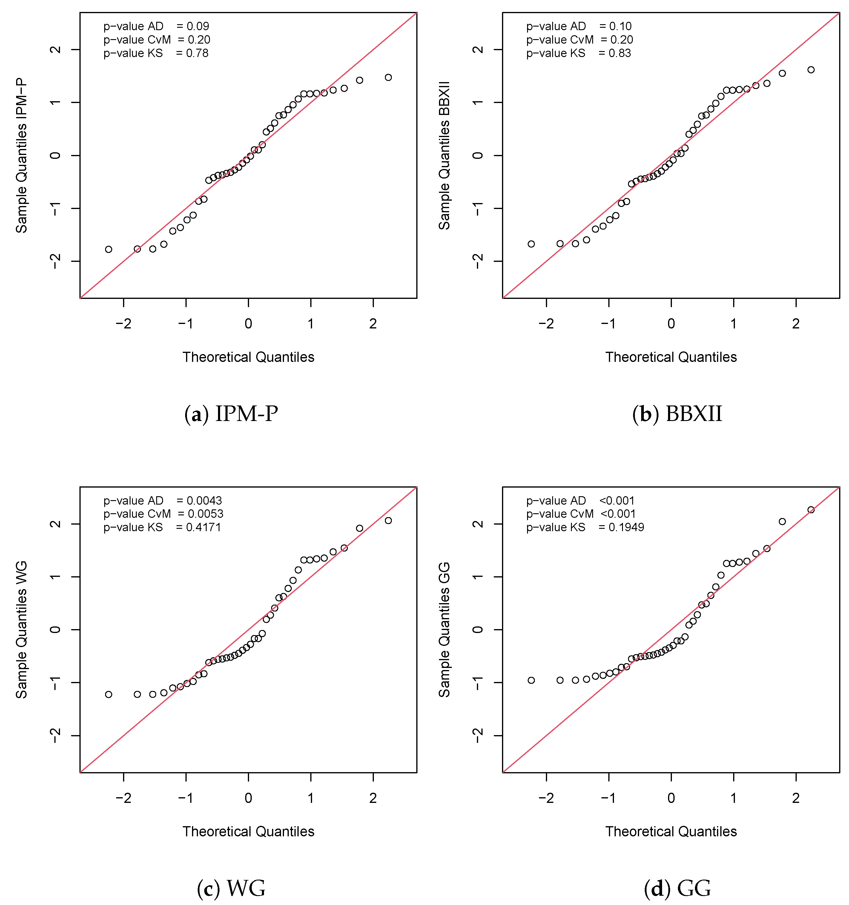
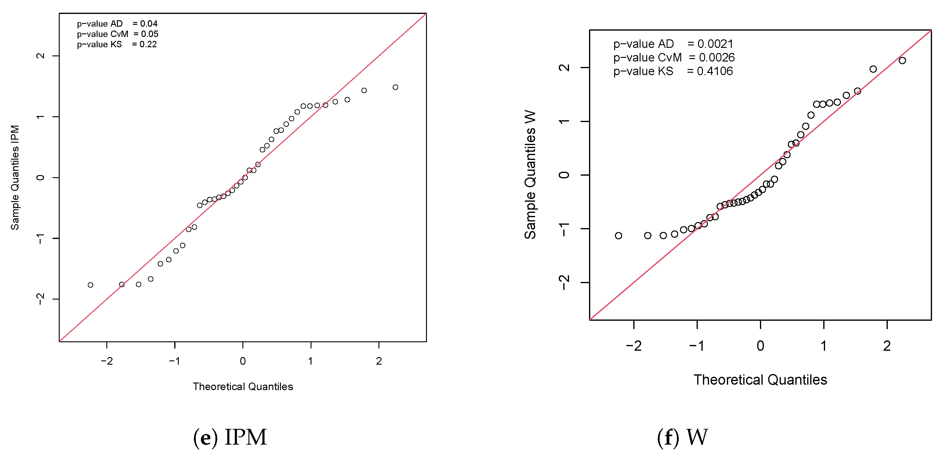
Figure 7 presents the QQ-plot for the QR in the IPM-P model and the p-values for the normality tests, suggesting that these residuals satisfy the assumption of normality and therefore, the IPM-P distribution is suitable for this dataset.
6. Conclusions
This paper has introduced the IPM-PS distribution, which is a composition between the IPM and PS models. We have also considered the Bell distribution, which has not been used as much in the literature as the Poisson, geometric or logarithmic distributions in the same context. Some of its most relevant properties were also studied, such as the PDF, the survival and hazard functions, and the moments. Parameter estimation was performed by the ML method using the EM algorithm. We highlight the implementation of the EM algorithm to perform the parameter estimation for the model, because it provides robustness in obtaining the maximum-likelihood estimators. We also emphasize the use of Oakes’ method to compute the hessian matrix of the model, because it provides an exact method and not an approximation of said matrix, as it is usually used. In addition, a simulation study was carried out showing the good statistical properties of these estimators in finite samples. As applications, two real datasets on the failure of an article and the measurement of BMI were considered. Several common models that are PS-based, such as the WPS and GPS, were also considered. Applying traditional information criteria, we have shown that our proposal provides a suitable alternative to model positive data. In addition to the possible interpretability of the model in terms of a competitive risk scheme, the model proved to be more useful in terms of precision compared to other usual alternatives in the literature. Therefore, it is of interest to disseminate the use and applications of this model. Further research could take into account the competitive risk structure of the IPM-PS model. For instance, by adding the case in Equation (1), a new cure rate model could be proposed similar to the recent work of Vásquez et al. [33] and Azimi et al. [34]. In such a case, the distribution of susceptible individuals is given by the IPM-PS distribution. An alternative way to extend this proposal would be to modify the PS distribution for M in Equation (1), e.g., using the COM-Poisson [35] or the modified PS model [36], which is a generalization of the PS class of distributions.
Author Contributions
Conceptualization, L.B.-B. and D.I.G.; methodology, L.B.-B., D.I.G. and H.J.G.; software, L.B.-B.; validation, D.I.G., H.J.G. and M.B.; formal analysis, L.B.-B., D.I.G. and H.J.G.; investigation, L.B.-B., D.I.G., H.J.G. and M.B.; resources, H.J.G. and M.B.; writing—original draft preparation, L.B.-B. and D.I.G.; writing—review and editing, H.J.G. and M.B.; supervision, D.I.G. All authors have read and agreed to the published version of the manuscript.
Funding
The research of Leonardo Barrios-Blanco was supported by Vicerrectoría de Investigación y Postgrado de la Universidad de Atacama.
Institutional Review Board Statement
Not applicable.
Informed Consent Statement
Not applicable.
Data Availability Statement
The data used in Section 5 were duly referenced.
Conflicts of Interest
The authors declare no conflict of interest.
Appendix A. Additional Plots
Figure A1.
PDF and hazard function for the IPM-G distribution, with .

Figure A2.
PDF and hazard function for the IPM-L distribution, with .

Appendix B. Explicit form for the Integral in u(r) of r-th Moment of the IPM- PS
Such integrals should be computed numerically. For instance, in R [28] using the integrate function.
Appendix C. Explicit form for the Integral in Equation (9) for the Shannon Entropy
Appendix D. Inverse and Derivatives of A(·)
Appendix E. Oakes’ Method for the IMP-PS Distribution
The standard errors can be calculated as the square root of the diagonal elements of the inverse of the Fisher information matrix, i.e.,
where the Fisher information matrix is given by , l is the observed log-likelihood function and .
Then, the formula for calculating the standard errors by the Oakes method [23] is defined as
where Q is the Q-function.
In this way, with the estimation of the parameters, they are substituted in the respective derivatives to obtain the Fisher information matrix to obtain the standard errors. The following are the calculations of the derivatives necessary to find this matrix.
Appendix E.1. Double Derivatives of the Function Q in Relation to the Parameters ζ
Appendix E.2. Double Derivatives of Function Q in Relation to Parameters and Expectation Mi
(Geometric)
(Poisson)
(Bell)
(Logarithmic)
where
Appendix F. PDF of Distributions Used in Applications
The PDF of the Gompertz power series distribution is given by
where , and .
The PDF of the Weibull power series distribution is given by
where , and .
The PDF of the Beta Burr XII distribution is given by
where is the beta function and , , , , and .
References
- Mahmoudi, E.; Jafari, A.A. The compound class of linear failure rate-power series distributions: Model, properties, and applications. Commun.-Stat.-Simul. Comput. 2017, 46, 1414–1440. [Google Scholar] [CrossRef]
- Silva, R.B.; Bourguignon, M.; Dias, C.R.; Cordeiro, G.M. The compound class of extended Weibull power series distributions. Comput. Stat. Data Anal. 2013, 58, 352–367. [Google Scholar] [CrossRef]
- Jafari, A.A.; Tahmasebi, S. Gompertz-power series distributions. Commun.-Stat.-Theory Methods 2016, 45, 3761–3781. [Google Scholar] [CrossRef]
- Silva, R.B.; Cordeiro, G.M. The Burr XII power series distributions: A new compounding family. Braz. J. Probab. Stat. 2015, 29, 565–589. [Google Scholar] [CrossRef]
- Shafiei, S.; Darijani, S.; Saboori, H. Inverse Weibull power series distributions: Properties and applications. J. Stat. Comput. Simul. 2016, 86, 1069–1094. [Google Scholar] [CrossRef]
- Elbatal, I.; Zayedm, M.; Rasekhi, M. The Exponential Pareto Power Series Distribution: Theory and Applications. Pak. J. Stat. Oper. Res. 2017, 13, 603–615. [Google Scholar] [CrossRef]
- Shekari, M.; Zamani, H.; Saber, M.M. The compound class of Janardan-power series distributions: Properties and applications. J. Data Sci. 2019, 17, 259–278. [Google Scholar] [CrossRef]
- Jordanova, P.; Petrova, M.; Stehlik, M. Compound power series distribution with negative multinomial summands: Characterisation and risk process. Revstat 2020, 18, 47–69. [Google Scholar]
- Elbatal, I.; Altun, E.; Afify, A.Z.; Ozel, G. The Generalized Burr XII Power Series Distributions with Properties and Applications. Ann. Data Sci. 2019, 6, 571–597. [Google Scholar] [CrossRef]
- Rivera, P.A.; Calderín-Ojeda, E.; Gallardo, D.I.; Gómez, H.W. A Compound Class of the Inverse Gamma and Power Series Distributions. Symmetry 2021, 13, 1328. [Google Scholar] [CrossRef]
- Shakhatreh, M.K.; Dey, S.; Kumar, D. Inverse Lindley power series distributions: A new compounding family and regression model with censored data. J. Appl. Stat. 2022, 49, 3451–3476. [Google Scholar] [CrossRef]
- Hassan, A.S.; Almetwally, E.M.; Gamoura, S.C.; Metwally, A.S. Inverse Exponentiated Lomax Power Series Distribution: Model, Estimation, and Application. J. Math. 2022, 2022, 1998653. [Google Scholar] [CrossRef]
- Aldahlan, M.A.; Jamal, F.; Chesneau, C.; Elbatal, I.; Elgarhy, M. Exponentiated power generalized Weibull power series family of distributions: Properties, estimation and applications. PLoS ONE 2020, 15, e0230004. [Google Scholar] [CrossRef]
- Chesneau, C.; Agiwal, V. Statistical theory and practice of the inverse power Muth distribution. J. Comput. Math. Data Sci. 2021, 1, 100004. [Google Scholar] [CrossRef]
- Noak, A. A class of random variable with discrete distribution. Ann. Inst. Stat. Math. 1950, 21, 127–132. [Google Scholar] [CrossRef]
- Jodrá, P.; Gómez, H.W.; Jiménez-Gamero, M.D.; Alba-Fernández, M.V. The power muth distribution. Math. Model. Anal. 2017, 22, 186–201. [Google Scholar] [CrossRef]
- Muth, E.J. Reliability models with positive memory derived from the mean residual life function. Theory Appl. Reliab. 1977, 2, 401–435. [Google Scholar]
- Singh, S.V.; Elgarhy, M.; Ahmad, Z.; Sharma, V.K.; Hamedani, G.G. New Class of Probability Distributions Arising from Teissier Distribution. In Mathematical Modeling, Computational Intelligence Techniques, and Renewable Energy. Advances in Intelligent Systems and Computing; Springer: Singapore, 2021; Volume 1287. [Google Scholar]
- Abdullah, A.M.; Elgarhy, M. A new Muth generated family of distributions with applications. J. Nonlinear Sci. Appl. 2018, 11, 1171–1184. [Google Scholar]
- Almarashi, M.; Jamal, F.; Chesneau, C.; Elgarhy, M. A new truncated Muth generated family of distributions with applications. Complexity 2021, 2021, 1211526. [Google Scholar] [CrossRef]
- Georg, M. LambertW: An R package for Lambert W x F Random Variables. In R Package Version 0.6.6.; R Foundation for Statistical Computing: Vienna, Austria, 2020. [Google Scholar]
- Dempster, A.P.; Laird, N.M.; Rubin, D.B. Maximum likelihood from incomplete data via the EM algorithm. J.R. Stat. Soc. Ser. 1977, 39, 1–22. [Google Scholar]
- Oakes, D. Direct calculation of the information matrix via the EM algorithm. J.R. Stat. Soc. 1999, 61, 479–482. [Google Scholar] [CrossRef]
- Raqab, M.Z.; Kundu, D.; Al-Awadhi, F.A. Compound zero-truncated Poisson normal distribution and its applications. Commun.-Stat.-Theory Methods 2021, 50, 3030–3050. [Google Scholar] [CrossRef]
- Shannon, C.E. A Mathematical Theory of Communication. Bell Syst. Technol. J. 1948, 27, 379–423. [Google Scholar] [CrossRef]
- Gallardo, D.I.; Romeo, J.S.; Meyer, R. A simplified estimation procedure based on the EM algorithm for the power series cure rate model. Commun. Stat.-Simul. Comput. 2017, 46, 6342–6359. [Google Scholar] [CrossRef]
- Jo, S.; Choi, T.; Park, B.; Lenk, P. bsamGP: An R Package for Bayesian Spectral Analysis Models Using Gaussian Process Priors. J. Stat. Softw. 2019, 90, 1–41. [Google Scholar] [CrossRef]
- R Core Team. R: A Language and Environment for Statistical Computing; R Foundation for Statistical Computing: Vienna, Austria, 2022; Available online: https://www.R-project.org/ (accessed on 3 March 2023).
- Akaike, H. A new look at the statistical model identification. IEEE Trans. Autom. Control 1974, 1, 716–723. [Google Scholar] [CrossRef]
- Schwarz, G. Estimating the dimension of a model. Ann. Stat. 1978, 6, 461–464. [Google Scholar] [CrossRef]
- Dunn, P.K.; Smyth, G.K. Randomized quantile residuals. J. Comput. Graph. Stat. 1996, 5, 236–244. [Google Scholar]
- Murthy, D.P.; Xie, M.; Jiang, R. Weibull Models; Wiley & Sons, Incorporated, John: Hoboken, NJ, USA, 2003. [Google Scholar]
- Vásquez, J.K.J.; Rodrigues, J.; Balakrishnan, N. A useful variance decomposition for destructive Waring regression cure model with an application to HIV data. Commun. Stat.-Theory Methods 2022, 51, 6978–6989. [Google Scholar] [CrossRef]
- Azimi, R.; Esmailian, M.; Gallardo, D.I.; Gómez, H.J. A New Cure Rate Model Based on Flory–Schulz Distribution: Application to the Cancer Data. Mathematics 2022, 10, 4643. [Google Scholar] [CrossRef]
- Conway, R.W.; Maxwell, W.L. A queuing model with state dependent services rates. J. Ind. Eng. 1962, 12, 132–136. [Google Scholar]
- Consul, P.C.; Famoye, F. Lagrangian Probability Distributions; Birkhäuser: Boston, MA, USA, 2006. [Google Scholar]
Figure 1.
PDF and hazard function for the IPM-P distribution with .

Figure 2.
PDF and hazard function for the IPM-B distribution with .

Figure 3.
EM algorithm scheme for the IPM-PS distribution.

Figure 4.
PDF of the IPM-B, WP, GP, and W models on the IMC dataset (left panel) and the empirical CDF compared with the estimated CDF for the same models (right panel).
Figure 4.
PDF of the IPM-B, WP, GP, and W models on the IMC dataset (left panel) and the empirical CDF compared with the estimated CDF for the same models (right panel).

Figure 5.
QQ plot for the QR for the IPM-B, BBXII, WP, GP, IPM, and W distributions for the beta-carotene data.
Figure 5.
QQ plot for the QR for the IPM-B, BBXII, WP, GP, IPM, and W distributions for the beta-carotene data.


Figure 6.
PDF of IPM-P, WG, GP, GG, IPM, and W models for failure time dataset (left panel) and the empirical CDF versus the estimated CDF for the same models (right panel).
Figure 6.
PDF of IPM-P, WG, GP, GG, IPM, and W models for failure time dataset (left panel) and the empirical CDF versus the estimated CDF for the same models (right panel).

Figure 7.
QQ plot of the QR for IPM-P, BBXII, WG, GG, IPM, and W distributions for the failure time dataset.
Figure 7.
QQ plot of the QR for IPM-P, BBXII, WG, GG, IPM, and W distributions for the failure time dataset.


Table 1.
Special cases of the distribution.
| Distribution | Notation | |||
|---|---|---|---|---|
| Geometric | Geo | 1 | ||
| Poisson | Po | |||
| Bell | Be | |||
| Logarithmic | Lo |
Table 2.
First and second moments and variance of the IPM-PS distribution, with and .
| IPM-G | |||||||||
|---|---|---|---|---|---|---|---|---|---|
| (0.1;−1) | (0.2;−1) | (0.5;−1) | (0.1;0.5) | (0.2;0.5) | (0.5;0.5) | (0.1;1) | (0.2;1) | (0.5;1) | |
| 1.4953 | 1.3291 | 0.8307 | 1.0860 | 0.9654 | 0.6034 | 0.9569 | 0.8505 | 0.5316 | |
| 3.7277 | 3.3135 | 2.0710 | 1.7405 | 1.5471 | 0.9670 | 1.0671 | 0.9485 | 0.5928 | |
| V | 1.4919 | 1.5470 | 1.3809 | 0.5611 | 0.6152 | 0.6029 | 0.1515 | 0.2251 | 0.3102 |
| IPM-L | |||||||||
| 1.5769 | 1.4891 | 1.1984 | 1.1453 | 1.0815 | 0.8705 | 1.0091 | 0.9529 | 0.7669 | |
| 3.9312 | 3.7123 | 2.9878 | 1.8355 | 1.7333 | 1.3950 | 1.1253 | 1.0627 | 0.8553 | |
| V | 1.4447 | 1.4950 | 1.5515 | 0.5238 | 0.5636 | 0.6373 | 0.1070 | 0.1546 | 0.2671 |
| IPM-P | |||||||||
| (0.1;−1) | (0.5;−1) | (2;−1) | (0.1;0.5) | (0.5;0.5) | (2;0.5) | (0.1;1) | (0.5;1) | (2;1) | |
| 1.5797 | 1.2805 | 0.5201 | 1.1474 | 0.9301 | 0.3777 | 1.0109 | 0.8194 | 0.3328 | |
| 3.9383 | 3.1924 | 1.2966 | 1.8388 | 1.4906 | 0.6054 | 1.1273 | 0.9138 | 0.3711 | |
| V | 1.4428 | 1.5527 | 1.0261 | 0.5224 | 0.6255 | 0.4627 | 0.1054 | 0.2423 | 0.2604 |
| IPM-B | |||||||||
| 1.4981 | 0.9098 | 0.0056 | 1.0881 | 0.6608 | 0.0041 | 0.9587 | 0.5822 | 0.0036 | |
| 3.7348 | 2.2681 | 0.0139 | 1.7438 | 1.0590 | 0.0065 | 1.0691 | 0.6492 | 0.0040 | |
| V | 1.4905 | 1.4404 | 0.0139 | 0.5599 | 0.6224 | 0.0065 | 0.1500 | 0.3103 | 0.0040 |
Table 3.
Simulation study using the EM algorithm for the IPM-G with 1000 replicates. For all the cases .
Table 3.
Simulation study using the EM algorithm for the IPM-G with 1000 replicates. For all the cases .
| True Value | |||||||||||||||
|---|---|---|---|---|---|---|---|---|---|---|---|---|---|---|---|
| bias | RMSE | SE | CP | bias | RMSE | SE | CP | bias | RMSE | SE | CP | ||||
| 0.5 | 1 | 0.5 | −0.0783 | 0.2152 | 0.7088 | 0.9310 | −0.0516 | 0.1879 | 0.5608 | 0.9570 | −0.0270 | 0.1543 | 0.3481 | 0.9660 | |
| 0.1415 | 0.3005 | 0.3507 | 0.9830 | 0.0851 | 0.2266 | 0.3132 | 0.9770 | 0.0366 | 0.1552 | 0.2365 | 0.9600 | ||||
| 0.0542 | 0.1328 | 0.3841 | 0.9990 | 0.0315 | 0.0887 | 0.2806 | 0.9700 | 0.0115 | 0.0490 | 0.1764 | 0.9660 | ||||
| −0.0336 | 0.1055 | 0.5604 | 0.9990 | −0.0156 | 0.0583 | 0.4467 | 0.9870 | −0.0012 | 0.0152 | 0.2789 | 0.9700 | ||||
| 0.2 | 0.0432 | 0.2111 | 0.7731 | 0.9770 | 0.0404 | 0.1643 | 0.5337 | 0.9710 | 0.0244 | 0.1133 | 0.4813 | 0.9650 | |||
| 0.0291 | 0.2075 | 0.3240 | 0.9870 | 0.0036 | 0.1581 | 0.2447 | 0.9710 | −0.0144 | 0.1000 | 0.2726 | 0.9660 | ||||
| 0.0717 | 0.1825 | 0.3119 | 0.9800 | 0.0427 | 0.1368 | 0.2091 | 0.9770 | 0.0049 | 0.0633 | 0.1412 | 0.9660 | ||||
| −0.0824 | 0.1625 | 0.7174 | 0.9800 | −0.0530 | 0.1189 | 0.5045 | 0.9770 | −0.0118 | 0.0438 | 0.4565 | 0.9600 | ||||
| 0.1 | 0.0318 | 0.3060 | 0.7434 | 0.9910 | 0.0370 | 0.1503 | 0.5364 | 0.9820 | 0.0224 | 0.0873 | 0.3129 | 0.9740 | |||
| 0.0220 | 0.1894 | 0.3427 | 0.9900 | −0.0004 | 0.1342 | 0.1942 | 0.9820 | −0.0149 | 0.0793 | 0.1091 | 0.9690 | ||||
| 0.1113 | 0.2970 | 0.2888 | 0.9950 | 0.0495 | 0.1596 | 0.2069 | 0.9910 | 0.0049 | 0.0714 | 0.1289 | 0.9790 | ||||
| −0.1054 | 0.1927 | 0.8066 | 0.9850 | −0.0620 | 0.1356 | 0.5439 | 0.9810 | −0.0157 | 0.0545 | 0.3312 | 0.9740 | ||||
| −0.2 | −0.0930 | 0.5089 | 0.9152 | 0.9920 | −0.3430 | 0.3655 | 0.6773 | 0.8670 | −0.0577 | 0.1943 | 0.4614 | 0.9770 | |||
| −0.0131 | 0.1356 | 0.5921 | 0.9820 | −0.0122 | 0.0952 | 0.4580 | 0.9770 | −0.0102 | 0.0600 | 0.1467 | 0.9690 | ||||
| 0.1882 | 0.5432 | 0.3252 | 0.9870 | 0.6742 | 0.5457 | 0.2439 | 0.9790 | 0.0299 | 0.1385 | 0.1670 | 0.9670 | ||||
| −0.0843 | 0.2032 | 1.5664 | 0.9870 | −0.0321 | 0.1230 | 1.2458 | 0.9790 | −0.0027 | 0.0490 | 0.6344 | 0.9690 | ||||
| 2 | 0.5 | −0.0806 | 0.2093 | 0.6795 | 0.9480 | −0.0514 | 0.1836 | 0.5117 | 0.9580 | −0.0259 | 0.1457 | 0.3659 | 0.9640 | ||
| 0.1295 | 0.3017 | 0.3595 | 0.9480 | 0.0793 | 0.2278 | 0.2954 | 0.9570 | 0.0306 | 0.1502 | 0.2486 | 0.9610 | ||||
| 0.0753 | 0.3383 | 0.3635 | 0.9810 | 0.0493 | 0.2218 | 0.2676 | 0.9770 | 0.0130 | 0.1080 | 0.1768 | 0.9640 | ||||
| −0.0298 | 0.1464 | 1.0769 | 0.9710 | −0.0147 | 0.0859 | 0.8224 | 0.9680 | −0.0026 | 0.0273 | 0.5823 | 0.9610 | ||||
| 0.2 | 0.0740 | 0.2136 | 0.7317 | 0.9840 | 0.0601 | 0.1733 | 0.5319 | 0.9720 | 0.0357 | 0.1092 | 0.3357 | 0.9620 | |||
| −0.0043 | 0.2099 | 0.3093 | 0.9940 | −0.0331 | 0.1597 | 0.2420 | 0.9800 | −0.0301 | 0.0960 | 0.1545 | 0.9773 | ||||
| 0.1360 | 0.4811 | 0.2876 | 0.9990 | 0.0386 | 0.3577 | 0.2110 | 0.9840 | 0.0117 | 0.1953 | 0.1302 | 0.9730 | ||||
| −0.1161 | 0.2187 | 1.3044 | 0.9890 | −0.0635 | 0.1622 | 1.0014 | 0.9810 | −0.0307 | 0.0906 | 0.6472 | 0.9790 | ||||
| 0.1 | 0.0607 | 0.2558 | 0.7508 | 0.9820 | 0.0583 | 0.1669 | 0.5352 | 0.9750 | 0.0319 | 0.0834 | 0.3194 | 0.9610 | |||
| −0.0236 | 0.1883 | 0.2961 | 0.9880 | −0.0389 | 0.1417 | 0.1934 | 0.9850 | −0.0369 | 0.0802 | 0.1125 | 0.9770 | ||||
| 0.1271 | 0.5441 | 0.2831 | 0.9900 | 0.0454 | 0.3748 | 0.2013 | 0.9850 | −0.0184 | 0.2258 | 0.1271 | 0.9710 | ||||
| −0.1214 | 0.2400 | 1.4822 | 0.9900 | −0.0758 | 0.1800 | 1.0671 | 0.9850 | −0.0251 | 0.1043 | 0.6699 | 0.9700 | ||||
Table 4.
Simulation study using the EM algorithm for the IPM-P with 1000 replicates. For all the cases .
Table 4.
Simulation study using the EM algorithm for the IPM-P with 1000 replicates. For all the cases .
| True Value | |||||||||||||||
|---|---|---|---|---|---|---|---|---|---|---|---|---|---|---|---|
| bias | RMSE | SE | CP | bias | RMSE | SE | CP | bias | RMSE | SE | CP | ||||
| 0.5 | 1 | 0.5 | −0.0622 | 0.2006 | 1.9905 | 0.9560 | −0.0363 | 0.1847 | 1.6212 | 0.9370 | −0.0024 | 0.1493 | 1.2423 | 0.9250 | |
| 0.0651 | 0.2493 | 0.3158 | 0.9810 | 0.0375 | 0.1969 | 0.2600 | 0.9750 | 0.0091 | 0.1452 | 0.2192 | 0.9640 | ||||
| −0.0147 | 0.1516 | 0.3144 | 0.9950 | −0.0107 | 0.1141 | 0.2390 | 0.9880 | −0.0007 | 0.0612 | 0.1604 | 0.9600 | ||||
| 0.2062 | 0.6869 | 0.3978 | 0.9970 | 0.1358 | 0.4748 | 0.3247 | 0.9860 | 0.0308 | 0.2132 | 0.2472 | 0.9790 | ||||
| 1 | 1 | 0.5 | −0.0671 | 0.2085 | 1.9345 | 0.9780 | −0.0362 | 0.1757 | 1.5427 | 0.9680 | −0.0047 | 0.1427 | 1.1113 | 0.9630 | |
| 0.1230 | 0.2947 | 0.3180 | 0.9720 | 0.0747 | 0.2279 | 0.2599 | 0.9670 | 0.0300 | 0.1518 | 0.2044 | 0.9610 | ||||
| 0.0477 | 0.1797 | 0.3475 | 0.9990 | 0.0318 | 0.1319 | 0.2552 | 0.9890 | 0.0232 | 0.0788 | 0.1712 | 0.9750 | ||||
| −0.0689 | 0.7308 | 0.3882 | 0.9860 | −0.0660 | 0.5294 | 0.3077 | 0.9800 | −0.0733 | 0.2831 | 0.2201 | 0.9700 | ||||
| 2 | 1 | 0.5 | −0.0498 | 0.2110 | 1.9715 | 0.9890 | −0.0269 | 0.1836 | 1.4665 | 0.9790 | 0.0140 | 0.1499 | 0.9608 | 0.9620 | |
| 0.2355 | 0.4180 | 0.3275 | 0.9850 | 0.1689 | 0.3203 | 0.2734 | 0.9770 | 0.0789 | 0.2077 | 0.2061 | 0.9660 | ||||
| 0.1628 | 0.2579 | 0.4444 | 0.9910 | 0.1314 | 0.2060 | 0.3156 | 0.9800 | 0.0900 | 0.1405 | 0.2010 | 0.9690 | ||||
| −0.6167 | 1.0444 | 0.3925 | 0.9870 | −0.5380 | 0.8661 | 0.2884 | 0.9700 | −0.4140 | 0.6041 | 0.1868 | 0.9680 | ||||
| 0.2 | 0.0313 | 0.2495 | 2.3864 | 0.9870 | 0.0317 | 0.1588 | 1.8656 | 0.9750 | 0.0166 | 0.0944 | 1.1976 | 0.9690 | |||
| −0.0124 | 0.1935 | 0.3168 | 0.9740 | −0.0226 | 0.1509 | 0.2235 | 0.9640 | −0.0148 | 0.0916 | 0.1374 | 0.9600 | ||||
| −0.0050 | 0.2085 | 0.2938 | 0.9920 | −0.0132 | 0.1564 | 0.2118 | 0.9840 | −0.0053 | 0.0944 | 0.1310 | 0.9710 | ||||
| 0.0839 | 0.7085 | 0.6032 | 0.9760 | 0.0707 | 0.6137 | 0.4598 | 0.9690 | 0.0243 | 0.3381 | 0.2975 | 0.9600 | ||||
| 0.1 | −0.0712 | 2.0289 | 0.5630 | 0.9980 | 0.0211 | 0.4026 | 1.8901 | 0.9860 | 0.0226 | 0.0769 | 1.2122 | 0.9750 | |||
| −0.0311 | 0.1827 | 1.5422 | 0.9890 | −0.0362 | 0.1445 | 0.2628 | 0.9630 | −0.0223 | 0.0838 | 0.1108 | 0.9600 | ||||
| 0.1051 | 2.3623 | 0.2907 | 0.9860 | −0.0180 | 0.4423 | 0.2134 | 0.9720 | −0.0124 | 0.1098 | 0.1326 | 0.9630 | ||||
| 0.1186 | 0.8074 | 2.1261 | 0.9930 | 0.1449 | 0.7578 | 0.5784 | 0.9820 | 0.0339 | 0.4028 | 0.3221 | 0.9720 | ||||
| −0.2 | −0.4583 | 9.7743 | 2.7164 | 0.9830 | −0.4739 | 12.7700 | 2.1530 | 0.9730 | −0.0805 | 0.3246 | 1.5611 | 0.9640 | |||
| −0.0713 | 0.1657 | 0.8047 | 0.9920 | −0.0574 | 0.1282 | 0.5628 | 0.9700 | −0.0297 | 0.0823 | 0.2070 | 0.9640 | ||||
| 1.9332 | 44.2624 | 0.2751 | 0.9810 | 0.6835 | 19.8681 | 0.2140 | 0.9750 | 0.0041 | 0.3105 | 0.1543 | 0.9670 | ||||
| 0.4587 | 1.1872 | 1.5392 | 0.9350 | 0.3772 | 0.9874 | 1.1873 | 0.9480 | 0.2001 | 0.6025 | 0.5607 | 0.9680 | ||||
| 2 | 0.5 | −0.0590 | 0.2046 | 1.9976 | 0.9990 | −0.0304 | 0.1798 | 1.6217 | 0.9970 | −0.0080 | 0.1471 | 1.2477 | 0.9780 | ||
| 0.0573 | 0.2482 | 0.3209 | 0.9720 | 0.0264 | 0.1917 | 0.2614 | 0.9660 | 0.0030 | 0.1434 | 0.2185 | 0.9640 | ||||
| −0.0344 | 0.3092 | 0.3113 | 0.9710 | −0.0322 | 0.2375 | 0.2369 | 0.9630 | −0.0191 | 0.1419 | 0.1599 | 0.9600 | ||||
| 0.1937 | 0.6670 | 0.7954 | 0.9920 | 0.1345 | 0.4885 | 0.6508 | 0.9910 | 0.0442 | 0.2692 | 0.4960 | 0.9960 | ||||
| 0.2 | 0.0340 | 0.2413 | 2.4225 | 0.9990 | 0.0386 | 0.1560 | 1.8048 | 0.9970 | 0.0244 | 0.1040 | 1.2031 | 0.9750 | |||
| −0.0328 | 0.1934 | 0.3199 | 0.9900 | −0.0439 | 0.1442 | 0.2199 | 0.9800 | −0.0426 | 0.0997 | 0.1404 | 0.9750 | ||||
| −0.0440 | 0.4214 | 0.2895 | 0.9760 | −0.0698 | 0.3155 | 0.2063 | 0.9660 | −0.0712 | 0.2201 | 0.1306 | 0.9600 | ||||
| 0.1083 | 0.7683 | 1.2248 | 0.9900 | 0.0881 | 0.6356 | 0.8844 | 0.9890 | 0.0750 | 0.4350 | 0.5925 | 0.9770 | ||||
| 0.1 | 0.0424 | 0.3420 | 2.5115 | 0.9950 | 0.0432 | 0.1536 | 1.8904 | 0.9840 | 0.0251 | 0.0815 | 1.2635 | 0.9760 | |||
| −0.0544 | 0.1891 | 0.3697 | 0.9890 | −0.0615 | 0.1495 | 0.1969 | 0.9780 | −0.0453 | 0.0904 | 0.1155 | 0.9620 | ||||
| −0.0891 | 0.5873 | 0.2878 | 0.9760 | −0.1124 | 0.3823 | 0.2082 | 0.9690 | −0.0837 | 0.2395 | 0.1376 | 0.9600 | ||||
| 0.1957 | 0.9359 | 1.4253 | 0.9770 | 0.1527 | 0.7494 | 0.9803 | 0.9700 | 0.0904 | 0.4559 | 0.6600 | 0.9600 | ||||
Table 5.
Simulation study using the EM algorithm for the IPM-B with 1000 replicates. For all the cases .
Table 5.
Simulation study using the EM algorithm for the IPM-B with 1000 replicates. For all the cases .
| True Value | |||||||||||||||
|---|---|---|---|---|---|---|---|---|---|---|---|---|---|---|---|
| bias | RMSE | SE | CP | bias | RMSE | SE | CP | bias | RMSE | SE | CP | ||||
| 0.5 | 1 | 0.5 | −0.0647 | 0.2052 | 0.8458 | 0.9460 | −0.0478 | 0.1802 | 0.6633 | 0.9590 | −0.0147 | 0.1416 | 0.4704 | 0.9680 | |
| 0.1279 | 0.2899 | 0.3174 | 0.9810 | 0.0847 | 0.2194 | 0.2624 | 0.9700 | 0.0290 | 0.1470 | 0.2165 | 0.9660 | ||||
| 0.0497 | 0.1415 | 0.3509 | 0.9860 | 0.0337 | 0.1005 | 0.2645 | 0.9770 | 0.0138 | 0.0524 | 0.1724 | 0.9660 | ||||
| −0.0459 | 0.1832 | 0.4464 | 0.9800 | −0.02568 | 0.1092 | 0.3532 | 0.9700 | −0.0096 | 0.0355 | 0.2483 | 0.9660 | ||||
| 1 | 1 | 0.5 | −0.0847 | 0.2197 | 0.6442 | 0.9140 | −0.0610 | 0.1796 | 0.4419 | 0.9320 | −0.0410 | 0.1520 | 0.2637 | 0.9660 | |
| 0.3063 | 0.4903 | 0.3231 | 0.9410 | 0.1980 | 0.3386 | 0.2662 | 0.9530 | 0.1006 | 0.2180 | 0.2066 | 0.9650 | ||||
| 0.1920 | 0.2799 | 0.4858 | 0.9770 | 0.1303 | 0.1996 | 0.3501 | 0.9840 | 0.0621 | 0.1136 | 0.2256 | 0.9670 | ||||
| −0.2241 | 0.3527 | 0.4201 | 0.9980 | −0.1380 | 0.2337 | 0.3036 | 0.9720 | −0.0570 | 0.1193& | 0.1887 | 0.9670 | ||||
| 2 | 1 | 0.5 | −0.1390 | 0.2193 | 0.3709 | 0.9800 | −0.1131 | 0.2028 | 0.2551 | 0.9720 | −0.0769 | 0.1726 | 0.1665 | 0.9690 | |
| 0.4175 | 0.7326 | 0.7068 | 0.9720 | 0.2426 | 0.3786 | 0.6131 | 0.9750 | 0.1299 | 0.2173 | 0.5371 | 0.9690 | ||||
| 0.2107 | 0.3243 | 1.1496 | 0.9710 | 0.1259 | 0.1832 | 0.8568 | 0.9860 | 0.0606 | 0.0907 | 0.6019 | 0.9970 | ||||
| −0.1562 | 0.3359 | 0.4613 | 0.9520 | −0.0743 | 0.1487 | 0.3479 | 0.9600 | −0.0249 | 0.0592 | 0.2285 | 0.9670 | ||||
| 0.2 | 0.0480 | 0.2630 | 0.9211 | 0.9830 | 0.0406 | 0.1583 | 0.6999 | 0.9710 | 0.0302 | 0.1154 | 0.4400 | 0.9620 | |||
| 0.0248 | 0.2076 | 0.2906 | 0.9820 | 0.0048 | 0.1533 | 0.2014 | 0.9710 | −0.0150 | 0.1023 | 0.1310 | 0.9640 | ||||
| 0.0713 | 0.2349 | 0.3063 | 0.9820 | 0.0371 | 0.1427 | 0.2312 | 0.9710 | 0.0110 | 0.0792 | 0.1428 | 0.9690 | ||||
| −0.1069 | 0.2299 | 0.6043 | 0.9830 | −0.0648 | 0.1703 | 0.45543 | 0.9800 | −0.0273 | 0.0914 | 0.2912 | 0.9770 | ||||
| 0.1 | 0.0342 | 0.2980 | 1.0518 | 0.9850 | 0.0365 | 0.1766 | 0.7190 | 0.9830 | 0.0244 | 0.1115 | 0.4275 | 0.9790 | |||
| −0.0005 | 0.1861 | 0.3416 | 0.9920 | −0.0024 | 0.1333 | 0.1743 | 0.9830 | −0.0170 | 0.0828 | 0.0993 | 0.9770 | ||||
| 0.0662 | 0.2706 | 0.3296 | 0.9850 | 0.0390 | 0.1859 | 0.2283 | 0.9790 | 0.0079 | 0.1049 | 0.1405 | 0.9670 | ||||
| −0.0831 | 0.2456 | 0.8136 | 0.9990 | −0.0680 | 0.1914 | 0.5084 | 0.9940 | −0.0246 | 0.1092 | 0.3080 | 0.9870 | ||||
| −0.2 | −0.0708 | 0.5232 | 1.0911 | 0.9910 | −0.0421 | 0.3010 | 0.8699 | 0.9800 | −0.0405 | 0.1763 | 0.6136 | 0.9610 | |||
| −0.0469 | 0.1546 | 0.5067 | 0.9940 | −0.0306 | 0.1091 | 0.2603 | 0.9740 | −0.0168 | 0.0697 | 0.1356 | 0.9630 | ||||
| 0.0746 | 0.5990 | 0.3029 | 0.9890 | 0.0283 | 0.2960 | 0.2443 | 0.9740 | 0.0078 | 0.1507 | 0.1721 | 0.9670 | ||||
| 0.0228 | 0.3499 | 1.2728 | 0.9830 | 0.0135 | 0.2384 | 0.8195 | 0.9750 | 0.0152 | 0.1336 | 0.5331 | 0.9610 | ||||
| 2 | 0.5 | −0.0619 | 0.1945 | 0.8590 | 0.9980 | −0.0416 | 0.1753 | 0.6607 | 0.9890 | −0.0078 | 0.1412 | 0.4426 | 0.9990 | ||
| 0.1125 | 0.2791 | 0.3363 | 0.9330 | 0.0729 | 0.2173 | 0.2650 | 0.9420 | 0.0159 | 0.1457 | 0.2127 | 0.9620 | ||||
| 0.0729 | 0.3018 | 0.3538 | 0.9800 | 0.0496 | 0.2202 | 0.2627 | 0.9720 | 0.0111 | 0.1150 | 0.1710 | 0.9670 | ||||
| −0.0283 | 0.1944 | 0.9046 | 0.9700 | −0.0194 | 0.1299 | 0.7037 | 0.9890 | −0.0050 | 0.0526 | 0.4684 | 0.9620 | ||||
| 0.2 | 0.0729 | 0.2117 | 0.9636 | 0.9900 | 0.0547 | 0.1564 | 0.6760 | 0.9850 | 0.0360 | 0.1081 | 0.4496 | 0.9780 | |||
| −0.0273 | 0.1958 | 0.3055 | 0.9910 | −0.0261 | 0.1517 | 0.2120 | 0.9720 | −0.0333 | 0.0975 | 0.1393 | 0.9610 | ||||
| 0.0640 | 0.4303 | 0.3059 | 0.9920 | 0.0357 | 0.3279 | 0.2164 | 0.9830 | −0.0037 | 0.1831 | 0.1390 | 0.9680 | ||||
| −0.0937 | 0.2673 | 1.2401 | 0.9910 | −0.0715 | 0.2148 | 0.8714 | 0.9860 | −0.0324 | 0.1177 | 0.5893 | 0.9690 | ||||
| 0.1 | 0.0749 | 0.2478 | 0.9590 | 0.9990 | 0.0682 | 0.1670 | 0.6936 | 0.9880 | 0.0354 | 0.0876 | 0.4347 | 0.9720 | |||
| −0.0373 | 0.1903 | 0.3065 | 0.9910 | −0.0583 | 0.1447 | 0.1788 | 0.9840 | −0.0433 | 0.0885 | 0.1002 | 0.9730 | ||||
| 0.0770 | 0.4571 | 0.2880 | 0.9780 | −0.0244 | 0.3578 | 0.2171 | 0.9660 | −0.0335 | 0.2197 | 0.1390 | 0.9600 | ||||
| −0.1132 | 0.2756 | 1.3742 | 0.9970 | −0.0447 | 0.2279 | 0.9692 | 0.9870 | −0.0210 | 0.1420 | 0.6188 | 0.9670 | ||||
Table 6.
Simulation study using the EM algorithm for the IPM-L with 1000 replicates. For all the cases .
Table 6.
Simulation study using the EM algorithm for the IPM-L with 1000 replicates. For all the cases .
| True Value | |||||||||||||||
|---|---|---|---|---|---|---|---|---|---|---|---|---|---|---|---|
| bias | RMSE | SE | CP | bias | RMSE | SE | CP | bias | RMSE | SE | CP | ||||
| 0.5 | 1 | 0.5 | −0.0913 | 0.2344 | 1.3674 | 0.9830 | −0.0599 | 0.1952 | 1.0293 | 0.9730 | −0.0365 | 0.1549 | 0.6736 | 0.9620 | |
| 0.1068 | 0.2685 | 0.4348 | 0.9830 | 0.0550 | 0.2051 | 0.3611 | 0.9730 | 0.0148 | 0.1424 | 0.2791 | 0.9760 | ||||
| 0.0100 | 0.1186 | 0.3590 | 0.9830 | −0.0102 | 0.0794 | 0.2659 | 0.9710 | −0.0235 | 0.0514 | 0.1677 | 0.9660 | ||||
| −0.0437 | 0.1403 | 0.6819 | 0.9730 | −0.0199 | 0.0769 | 0.5082 | 0.9710 | −0.0102 | 0.0192 | 0.3254 | 0.9620 | ||||
| 0.2 | −0.3935 | 1.6522 | 1.3146 | 0.9740 | 0.0161 | 0.1571 | 0.9409 | 0.9700 | −0.0014 | 0.0963 | 0.6257 | 0.9640 | |||
| 0.0066 | 0.1899 | 0.6875 | 0.9910 | −0.0069 | 0.1390 | 0.2749 | 0.9820 | −0.0142 | 0.0852 | 0.1846 | 0.9740 | ||||
| 0.1861 | 1.6107 | 0.2626 | 0.9910 | −0.0048 | 0.1053 | 0.1808 | 0.9720 | −0.0271 | 0.0631 | 0.1135 | 0.9640 | ||||
| −0.1176 | 0.1962 | 0.9611 | 0.9940 | −0.0758 | 0.1442 | 0.5331 | 0.9800 | −0.0293 | 0.0677 | 0.3649 | 0.9740 | ||||
| 0.1 | 0.0042 | 0.4007 | 1.2466 | 0.9850 | 0.0154 | 0.1490 | 0.8994 | 0.9760 | 0.0025 | 0.0896 | 0.5491 | 0.9690 | |||
| 0.0016 | 0.1708 | 0.4576 | 0.9930 | −0.0082 | 0.1162 | 0.2241 | 0.9810 | −0.0163 | 0.0703 | 0.1307 | 0.9750 | ||||
| 0.0608 | 0.3558 | 0.2454 | 0.9850 | 0.0043 | 0.1201 | 0.1726 | 0.9760 | −0.0269 | 0.0726 | 0.1080 | 0.9650 | ||||
| −0.1368 | 0.2118 | 0.9204 | 0.9930 | −0.0904 | 0.1640 | 0.5495 | 0.9860 | −0.0351 | 0.0812 | 0.3475 | 0.9690 | ||||
| −0.2 | −0.8713 | 1.3807 | 1.3926 | 0.9870 | −0.1653 | 0.5025 | 1.0040 | 0.9720 | −0.1012 | 0.2560 | 0.6365 | 0.9610 | |||
| −0.0079 | 0.1100 | 1.2154 | 0.9850 | −0.0110 | 0.0795 | 0.4796 | 0.9770 | −0.0106 | 0.0525 | 0.1965 | 0.9960 | ||||
| 1.6920 | 3.4927 | 0.2594 | 0.9980 | 0.1181 | 0.4368 | 0.1866 | 0.9870 | 0.0243 | 0.1559 | 0.1196 | 0.9790 | ||||
| −0.1205 | 0.2113 | 1.3655 | 0.9870 | −0.0667 | 0.1424 | 1.1179 | 0.9770 | −0.0189 | 0.0593 | 0.5751 | 0.9690 | ||||
| 2 | 0.5 | −0.0965 | 0.2355 | 1.2621 | 0.9820 | −0.0541 | 0.1903 | 0.9674 | 0.9760 | −0.0320 | 0.1521 | 0.6883 | 0.9670 | ||
| 0.1020 | 0.2691 | 0.4254 | 0.9820 | 0.0378 | 0.2007 | 0.3501 | 0.9760 | 0.0082 | 0.1424 | 0.2801 | 0.9650 | ||||
| −0.0087 | 0.2752 | 0.3522 | 0.9720 | −0.0554 | 0.2024 | 0.2537 | 0.9690 | −0.0565 | 0.1107 | 0.1619 | 0.9650 | ||||
| −0.0279 | 0.1621 | 1.3228 | 0.9820 | −0.0034 | 0.1044 | 0.9964 | 0.9760 | −0.0076 | 0.0282 | 0.6670 | 0.9680 | ||||
| 0.2 | 0.0260 | 0.2239 | 1.2350 | 0.9890 | 0.0190 | 0.1622 | 0.9383 | 0.9750 | 0.1019 | 0.6279 | 0.6200 | 0.9690 | |||
| −0.0117 | 0.1867 | 0.3544 | 0.9870 | −0.0280 | 0.1361 | 0.2810 | 0.9750 | −0.0241 | 0.0879 | 0.1840 | 0.9670 | ||||
| −0.0061 | 0.3345 | 0.2585 | 0.9900 | −0.0570 | 0.2333 | 0.1800 | 0.9800 | −0.0743 | 0.1438 | 0.1147 | 0.9720 | ||||
| −0.1002 | 0.2056 | 1.4290 | 0.9870 | −0.0636 | 0.1509 | 1.0908 | 0.9700 | −0.0263 | 0.0760 | 0.7386 | 0.9690 | ||||
| 0.1 | 0.0180 | 0.2640 | 1.1769 | 0.9880 | 0.0133 | 0.1712 | 0.8844 | 0.9790 | 0.0022 | 0.0750 | 0.5468 | 0.9680 | |||
| −0.0212 | 0.1646 | 0.3278 | 0.9800 | −0.0311 | 0.1141 | 0.2360 | 0.9750 | −0.0263 | 0.0693 | 0.1289 | 0.9680 | ||||
| 0.0163 | 0.3927 | 0.2341 | 0.9830 | −0.0587 | 0.2823 | 0.1714 | 0.9780 | −0.0799 | 0.1674 | 0.1069 | 0.9680 | ||||
| −0.1189 | 0.2260 | 1.4648 | 0.9830 | −0.0674 | 0.1733 | 1.1255 | 0.9790 | −0.0305 | 0.0991 | 0.6944 | 0.9680 | ||||
Table 7.
Parameter estimation, standard errors (in parentheses), AIC and BIC comparison criteria for IMC values.
Table 7.
Parameter estimation, standard errors (in parentheses), AIC and BIC comparison criteria for IMC values.
| Distribution | IPM-B | GP | WP | BBXII | IPM | W |
|---|---|---|---|---|---|---|
| −12.610 (1.5148) | 0.0037 (1.1 ) | 5.3277 (0.0043) | 15.156 (1.2348) | 0.144 (0.253) | − | |
| 6.0506 (0.6685) | 0.1198 (2.9 ) | 0.0280 (6.7 ) | 0.9763 (0.6613) | 2.484 (0.505) | 4.169 (0.1610) | |
| 0.0660 (0.0143) | 0.0997 (0.4975) | 4.2861 (0.3996) | 14.812 (0.9717) | 1.075 (0.069) | 28.565 (0.4119) | |
| 0.0016 (0.5050) | − | − | 0.8248 (0.5488) | − | − | |
| − | − | − | 7.4191 (1.4849) | − | − | |
| AIC | 1909.79 | 2174.64 | 2012.36 | 1911.41 | 1913.79 | 2063.75 |
| BIC | 1924.79 | 2185.89 | 2023.61 | 1930.16 | 1926.82 | 2071.25 |
Table 8.
Point and interval estimation for the percentage of patients with overweight using different distributions.
Table 8.
Point and interval estimation for the percentage of patients with overweight using different distributions.
| Distribution | IBM | 95% CI | Interval Length |
|---|---|---|---|
| IPMB | 0.1910 | (0.1836–0.1985) | 0.0149 |
| BBXII | 0.1922 | (0.1847–0.1998) | 0.0151 |
| IPM | 0.1938 | (0.1763–0.2113) | 0.0175 |
| WP | 0.2364 | (0.2264–0.2464) | 0.0199 |
Table 9.
Parameter estimation, standard errors (in parentheses), AIC and BIC criteria for failure times of 40 articles.
Table 9.
Parameter estimation, standard errors (in parentheses), AIC and BIC criteria for failure times of 40 articles.
| Distribution | IPM-P | GG | WG | BBXII | IPM | W |
|---|---|---|---|---|---|---|
| 0.1398 (0.2946) | 0.0728 (0.3357) | 0.0078 (6.6 ) | 7.3236 (3.5 ) | 0.019 (0.041) | − | |
| 2.4751 (0.6374) | 1.6926 (0.0125) | 2.4962 (0.1401) | 11.366 (8.4 ) | 5.893 (0.309) | 2.3451 (0.2798) | |
| 1.0698 (0.2219) | 2.2587 (0.0225) | 0.9392 (0.0032) | 0.3442 (2.2 ) | 0.044 (0.001) | 1.3937 (0.0998) | |
| 0.0459 (1.9492) | − | − | 0.0673 (6.3 ) | − | − | |
| − | − | − | 6.3903 (3.8 ) | − | − | |
| AIC | 64.68 | 72.85 | 65.62 | 65.92 | 68.68 | 66.58 |
| BIC | 71.44 | 77.92 | 71.69 | 74.36 | 76.13 | 69.96 |
Disclaimer/Publisher’s Note: The statements, opinions and data contained in all publications are solely those of the individual author(s) and contributor(s) and not of MDPI and/or the editor(s). MDPI and/or the editor(s) disclaim responsibility for any injury to people or property resulting from any ideas, methods, instructions or products referred to in the content. |
© 2023 by the authors. Licensee MDPI, Basel, Switzerland. This article is an open access article distributed under the terms and conditions of the Creative Commons Attribution (CC BY) license (https://creativecommons.org/licenses/by/4.0/).
Share and Cite
MDPI and ACS Style
Barrios-Blanco, L.; Gallardo, D.I.; Gómez, H.J.; Bourguignon, M. A Compound Class of Inverse-Power Muth and Power Series Distributions. Axioms 2023, 12, 383. https://doi.org/10.3390/axioms12040383
AMA Style
Barrios-Blanco L, Gallardo DI, Gómez HJ, Bourguignon M. A Compound Class of Inverse-Power Muth and Power Series Distributions. Axioms. 2023; 12(4):383. https://doi.org/10.3390/axioms12040383
Chicago/Turabian StyleBarrios-Blanco, Leonardo, Diego I. Gallardo, Héctor J. Gómez, and Marcelo Bourguignon. 2023. "A Compound Class of Inverse-Power Muth and Power Series Distributions" Axioms 12, no. 4: 383. https://doi.org/10.3390/axioms12040383
Note that from the first issue of 2016, this journal uses article numbers instead of page numbers. See further details here.