Article

Mathematical Model to Calculate Heat Transfer in Cylindrical Vessels with Temperature-Dependent Materials

by
Martina Fernández-Gracía
1,
Juan Francisco Sánchez-Pérez
2,*,
Francisco del Cerro
1 and
Manuel Conesa
2
1
Department of Electromagnetism and Electronics, Universidad de Murcia, 30100 Murcia, Spain
2
Department of Applied Physics and Naval Technology, Universidad Politécnica de Cartagena (UPCT), Campus Alfonso XIII, 30203 Cartagena, Spain
*
Author to whom correspondence should be addressed.
Axioms 2023, 12(4), 335; https://doi.org/10.3390/axioms12040335
Submission received: 28 February 2023 / Revised: 23 March 2023 / Accepted: 28 March 2023 / Published: 29 March 2023
(This article belongs to the Special Issue Applied Mathematical Modeling and Optimization)

Abstract

:
In this article, a mathematical model capable of simulating the heat transfer of cylindrical vessels whose properties are dependent on temperature is proposed. As a case study, it compares, from an approach of their heat transfer and chemical migration characteristics as a function of the temperature reached, different materials commonly used for the manufacture of water bottles. More specifically, the materials studied were aluminium, polyethylene terephthalate, and polypropylene. The validation of the model consists of an experiment carried out in the laboratory with three water bottles of each of the materials under study, as well as simulations using the Network Simulation Method to recreate the heat transfer that occurs through the walls of the bottles. On the other hand, the nondimensionalization technique is also applied, which allows us to obtain the weight of each of the variables on the problem, as well as the existing relationship between them. Finally, an outside temperature of 30 °C to 50 °C is simulated, which is a common temperature range in southern Europe during the summer season, and an initial temperature of 20 °C for the water contained in the bottle to know the behaviour of the materials and what the final temperature of the water would be after one hour.

1. Introduction

Traditionally in heat transfer problems, the properties of the materials have been considered constant depending on the material to be studied since, in many cases, there was no information available on how they varied as a function of temperature [1,2], but this does not adjust to the real behaviour of the materials, since if we vary the temperature to which the material is subjected, we can observe how the density, thermal conductivity and specific heat, among other properties, its value is altered [3,4,5,6,7,8].
This is why heat transfer problems that are usually carried out considering constant parameters include in their results an error due to the non-consideration of the variability of the properties with the increase or decrease of the temperature. These changes in properties affect the results derived from the heat transfer mechanisms, conduction, radiation and convection [9].
In this work, where the thermal behaviour of a vessel containing a fluid will be studied, as will be shown later, the main mechanisms of heat transfer that can occur are conduction and convection both in its own structure and with its environment, since heat transfer by radiation has been minimised.
The convection process requires the existence of a fluid capable of transporting thermal energy between two points where there is a temperature gradient. Considering that the fluid inside the vessel is at rest, the fluid in charge of transporting the thermal energy will be the moving air surrounding the vessel.
In the radiation process, the existence of an object that transmits heat or direct contact with the heat source is necessary, not generating thermal energy until the electromagnetic (infrared) waves are absorbed. Therefore, in case of application of this study (Section 6), the sun radiates these waves, which are received by the surface of the container which, by absorbing them, transforms them into thermal energy that will subsequently be transmitted to the internal fluid contained in the container through the processes of conduction and convection. For the validation of the proposed mathematical model, radiation to solar exposure will be minimised.
For heat transfer by conduction to exist, there must be a temperature gradient in the volume of a solid or between two materials in contact. In this case, there is a temperature gradient between the surface of the container and the fluid inside it. The transfer of this thermal energy will occur without the exchange of matter due to the vibrational motion of the atoms. As the temperature increases, the atoms will increase their velocity, colliding with neighbouring atoms and transferring this thermal energy to them.
Regarding the properties that influence the conduction mechanism, it is difficult to find conductivity values for many materials, such as some fluids or polymers, and moreover, in many of these cases, they usually present constant values [10]. However, more and more works present this property with temperature dependence [11,12,13,14,15,16], so it is necessary to introduce this variability of the properties with temperature in the mathematical models to improve the accuracy of the simulations.
The proposed mathematical model that will include the aforementioned heat transfer phenomena, as well as the variability of material properties with temperature, is simulated using the Network Simulation Method [9,17,18]. This method has been widely used in numerous problems applied to engineering [19,20], such as diffusion of chlorides in reinforced concrete [21], corrosion problems [22], soil consolidation [23], and solidification problems [24], among others. This model is validated through different experimental tests with three materials, aluminium 319 (Al319), polyethylene terephthalate (PET) and polypropylene (PP). Other authors have used other techniques to solve problems similar to the one posed in this article [25,26].
On the other hand, through the nondimensionalization technique, the relationship between the variables of the problem has been established, allowing us to know the influence of each one of them, as verified in the case study.
As an example of the study of the proposed mathematical model, the distribution of temperatures in bottles of different materials has been studied since the variation of temperatures in plastic materials could lead to an increase in the migration of substances into water [27,28] such as BPA, dimethyl phthalate (DMP), DEHP, OP, among others. Also, this article shows how properties vary as a function of temperature for aluminium 319, polyethylene (PET), and polypropylene (PP), materials commonly used in water bottles. In certain cases, some properties are not significantly affected by temperature, and it can be assumed that not considering the variability would not lead to substantial error, while other properties are affected to a greater extent causing a larger error if considered constant.
In summary, the main objective of this paper is to develop a mathematical model that includes the dependence, in many cases nonlinear, of the material properties on temperature, thus improving the accuracy of the simulations of the network model developed from the mathematical equations. It should be noted the sensitivity of the model to the variability of the properties with temperature is due to the strong coupling of the equations and the nonlinearity, so it is necessary to implement the properties of the materials with the best possible fit. Finally, a study has been added that indicates the weight of each of the variables on the proposed problem carried out using the nondimensionalization technique.

2. Mathematical Model

The mathematical model that is going to be described below is that of a cylinder that can be formed from different materials and whose properties vary with the temperature. As indicated above, the mechanisms to consider are conduction, convection, and radiation. In conduction processes, Fourier’s law is used to determine the heat transfer:
2 T x 2 + 2 T y 2 + 2 T z 2 = 1 α T t ;   α = k ρ   c e
where T is a temperature (K), α is thermal diffusivity (m2/s), k is thermal conductivity (W/mK), ce is specific heat capacity (J/kg K), ρ is density (kg/m3), t the time (s), and, finally x, y, z are the spatial coordinates. As previously indicated, the thermal conductivity, density, and specific heat capacity, and therefore the thermal diffusivity, will be expressed as a function of temperature.
Because the problem that we are going to develop is a cylindrical vessel, we are interested in defining the problem in cylindrical coordinates. The equation must be defined by the radius, r, the angle, φ, and the height, z, as follows, Figure 1:
1 r r k   r T r + 1 r 2 φ k T φ + z k T z = ρ   c e T t
Given the symmetry of the problem, it can be developed in two dimensions, radial and in height, showing the equation to which the network model will be developed, Equation (2):
1 r r k   r T r + z k T z = ρ   c e T t
If we develop the previous equation, it would be given by:
k r T r + k 2 T r 2 + k 2 T z 2 = ρ   c e T t
Finally, if we group the terms to facilitate the subsequent development of the network model, the equation would be given as follows:
1 r k ρ   c e T r + k ρ   c e 2 T r 2 + k ρ   c e 2 T z 2 = T t
It should be noted that the grouping of the properties will facilitate its subsequent development in the network model because, as previously indicated, its value depends on the temperature itself.
On the other hand, the implementation of the convection phenomenon is given by Newton’s law of cooling:
d Q d t = A h T s T e
where Q is the heat (J), h is the heat transfer coefficient (W/m2K), A is the heat transfer surface area (m2), Ts is the temperature of the solid surface (K), and finally, Te is the environmental temperature (K).
Finally, the phenomenon of radiation is given by Stefan–Boltzmann’s Law
d Q d t = ε σ T s 4 T e 4 · d S
where ε and σ are the emissivity and the Stefan–Boltzmann constant (W/m2K4), respectively.

3. Network Model

The Network Simulation Method is a method used to solve various physical-chemical processes that can be defined by a mathematical model. It consists of converting each one of the summands of the equation into an element of an electrical circuit, thus simulating, in this case, a problem of heat transmission through an electrical circuit. That is, an electrical analogy is established between the variables of the problem and the voltage in a central node. This equivalence has been used in heat transfer problems [29,30]; however, the resolution methodology is different. In this case, the proposed method has been widely used satisfactorily in numerous engineering problems [9,17,18].
Therefore, we must proceed to convert Equation (5) into terms that can be used for the Network Simulation Method. The term that appears by multiplying all the summands on the left-hand side of the equation can be expressed as thermal diffusivity, α, which is temperature dependent because its variables are temperature dependent. On the other hand, the terms of the second derivative, after some mathematical operations, will be implemented as two resistors in series.
1 r α T r + α 2 T r 2 + α 2 T z 2 = T t
As indicated, in order to implement the second derivatives as resistances, it is necessary that they be free of variable terms. To do this, they are separated into two addends (Equation (9)), where one, its electrical analogy, would be given by a voltage-controlled current generator, and the other, by two resistors in series.
α 2 T r 2 = α 1 2 T r 2 + 2 T r 2
Performing the same mathematical operation for the term 2 T z 2 , the equation is as follows:
1 r α T r + α 1 2 T r 2 + 2 T r 2 + α 1 2 T z 2 + 2 T z 2 = T t
On the one hand, any second partial derivative free of variable terms is identified in the circuit as two resistors in series. On the other hand, any second partial derivative or first partial derivative with multiplying dependent terms is identified in the circuit as voltage-controlled current sources, and finally, the time derivative represents in the circuit a capacitor. Therefore, for our circuit it would be as follows:
1 r   α T r , ( α 1 ) 2 T r 2 , ( α 1 ) 2 T z 2 are considered voltage-controlled current sources,
2 T z 2 , 2 T z 2 are considered as two resistors in a series,
T t represents a capacitor.
Taking into account that the terms that include α are temperature-dependent functions, voltage-controlled sources will be considered. Prior to the development of the network model, the expressions that include differential equations are spatially discretised by dividing the space into n volume elements according to Figure 2. Thus, the above equations can be expressed in finite differences. Finally, the centres of the cells are balanced with the electrical currents of each of the elements that make up the circuit.
Using the nomenclature of Figure 2, the spatial discretisation of the first and second derivatives is performed by balances between the central nodes and cell edges [30,31]. Thus, the first derivative in finite differences is given by:
T t = T i + 1 , j T i 1 , j Δ r
where Δ r = r i + 1 , j r i 1 , j and the second derivative by:
2 T z 2 = T i + 1 , j T i , j Δ r 2 T i , j T i 1 , j Δ r 2 Δ r = T i + 1 , j + T i - 1 , j 2 T i 1 , j Δ 2 r 2
where the expression (12) is the value of the resistance when implementing the electrical device
R = 1 Δ 2 r 2
Therefore, the circuit that would represent our problem, considering all of the above, would be the following, Figure 3:
Finally, the boundary conditions, radiation and convection, are implemented by means of a voltage-controlled current generator. The network model is simulated using circuit simulation software such as NgSpice [32].
The NgSpice software (version ngspice-39) [32] uses computational algorithms that allow solving electrical circuits derived from coupled and nonlinear mathematical models such as the one proposed in this article. These algorithms, derived from Nagel’s work [33], include Gear’s time fixation methods [34], trapezoidal integration [35], and the Runge–Kutta algorithm. The efficiency and precision are obtained by reducing the local truncation error and facilitating stability in the convergence of the numerical solution.

4. Nondimensionalization Technique

In this section, a study will be carried out on the behaviour of variables through their appraisal in dimensionless monomials. For this, the nondimensionalization technique will be used, which is a mathematical methodology that allows us to identify the monomials that control the problem posed [36,37,38]. The greatest difficulty that it presents is the correct choice of the reference variables, so it is necessary to have a deep knowledge of the problem posed. In addition, the technique of discrimination must be introduced, which introduces the variability of the properties in the different dimensions of space. Although the properties in the posed problem vary with temperature, it is going to be assumed that they are constant, a decision that we will justify at the end of the section, for the application of the nondimensionalization technique since it facilitates its application and, this study, is only intended to set how variables are grouped.
The first step is to establish the dimensionless variables that, thanks to the references used, will be in the range of [0–1], Equation (14).
T = T T i T e T i     r = r R     z = z H   t = t τ
where Ti is the initial temperature of the vessel, Te is room temperature, H is the height, and τ is the time at which the problem reaches a steady state. It should be noted that in the case of the radius, as shown in Figure 1, only the vessel structure without the fluid will be studied, R = r1 − r2, since it is where the heating of the container with the air is taking place, although the solution obtained will also be valid in the event that the entire cylinder is solid, R = r1. On the other hand, it should also be indicated that the study is being carried out with symmetry, and therefore, the results obtained will also be valid for the complete cylinder. Finally, the cylinder is considered to be heating since Te > Ti. In case it is cooling, Ti > Te, the procedure to be followed would be the same.
Next, the dimensionless variables are introduced in Equation (8) to obtain the dimensionless equation:
α T e T i R 2 1 r T r + α T e T i R 2 2 T r 2 + α T e T i H 2 2 T z 2 = T e T i τ T t
As expected, the range of variation does not depend on T’ [21]. Assuming that the changes of the derived factors in Equation (15) are of unit order of magnitude, the equation gives three coefficients, indicated in brackets, and these, two dimensionless monomials that must also be of unit order of magnitude, Equation (17).
α R 2   α H 2   1 τ
π 1 = α τ R 2   π 2 = R 2 H 2
where the monomial π1 represents the relationship of the temperature change with diffusion phenomena and the monomial π2 the geometric relationship of the dimensions of the cylinder.
Given that the test is realised under conditions where convection phenomena predominate, as previously indicated, if we apply the nondimensionalization technique to Equation (6), and knowing that d Q = ρ c e A R d T and α = k ρ c e two coefficients are obtained that provide the monomial π3.
α h R k   1 τ
π 3 = α h τ R k
Since the unknown τ appears in both the monomial π1 and π3, and it is interesting that it is only found in one of them, a new monomial can be obtained without this unknown by means of simple mathematical operations between both monomials.
π 4 = h R k
If symmetry had not been assumed, the π4 monomial would have been π 4 = h D k , where D is the cylinder diameter, which is the well-known Nusselt number, Nu, which relates the heat transfer coefficient, h, and the material thermal conductivity, k [39]. This same monomial could have been deduced by nondimensionalization from the equivalence between Equations (6) and (8) on the boundary [26].
Finally, the solution for the unknown τ, that is, the time in which the system reaches a steady state, can be deduced by applying the π-theorem, π1 = Ψ (π2, π4).
τ = R 2 α Ψ R 2 H 2 , h R k
where Ψ is an unknown function. Analysing Equation (21), and as in the case study, Section 6, the geometric variables, r1, r2 and H, will be the same for all materials. The speed at which the temperature increases for each of the vessels will depend on the thermal diffusivity, α, as expected, and on the relationship between the heat transfer coefficient, h, and the material thermal conductivity, k, that is, the Nusselt number. Finally, as previously indicated, the properties of the materials in this study depend on temperature, so this dependence should have been applied to the previous procedure. However, the relationships obtained between the properties of the materials would have been similar, being qualified by their dependence on temperature [21].

5. Material Properties and Model Validation

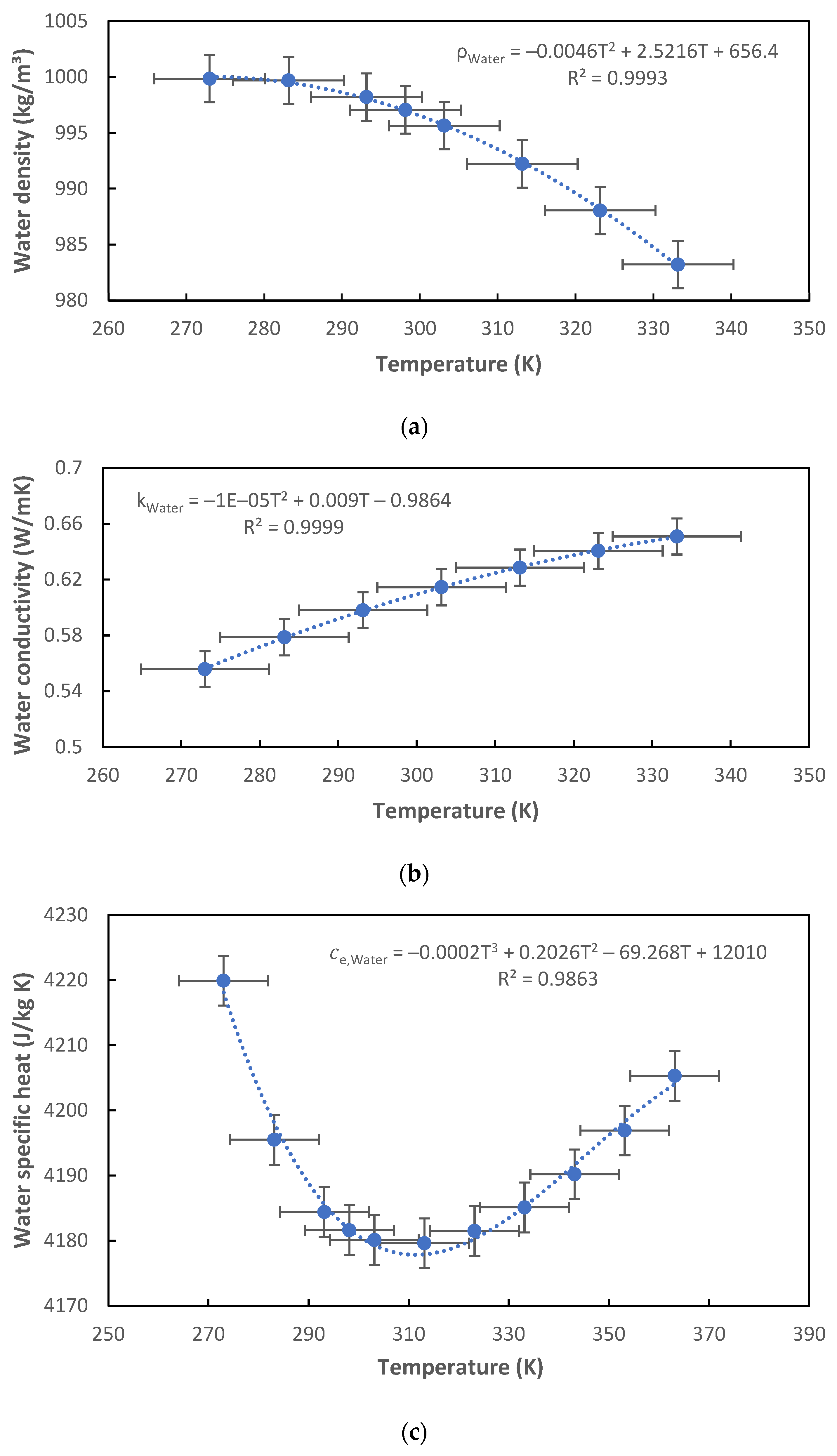
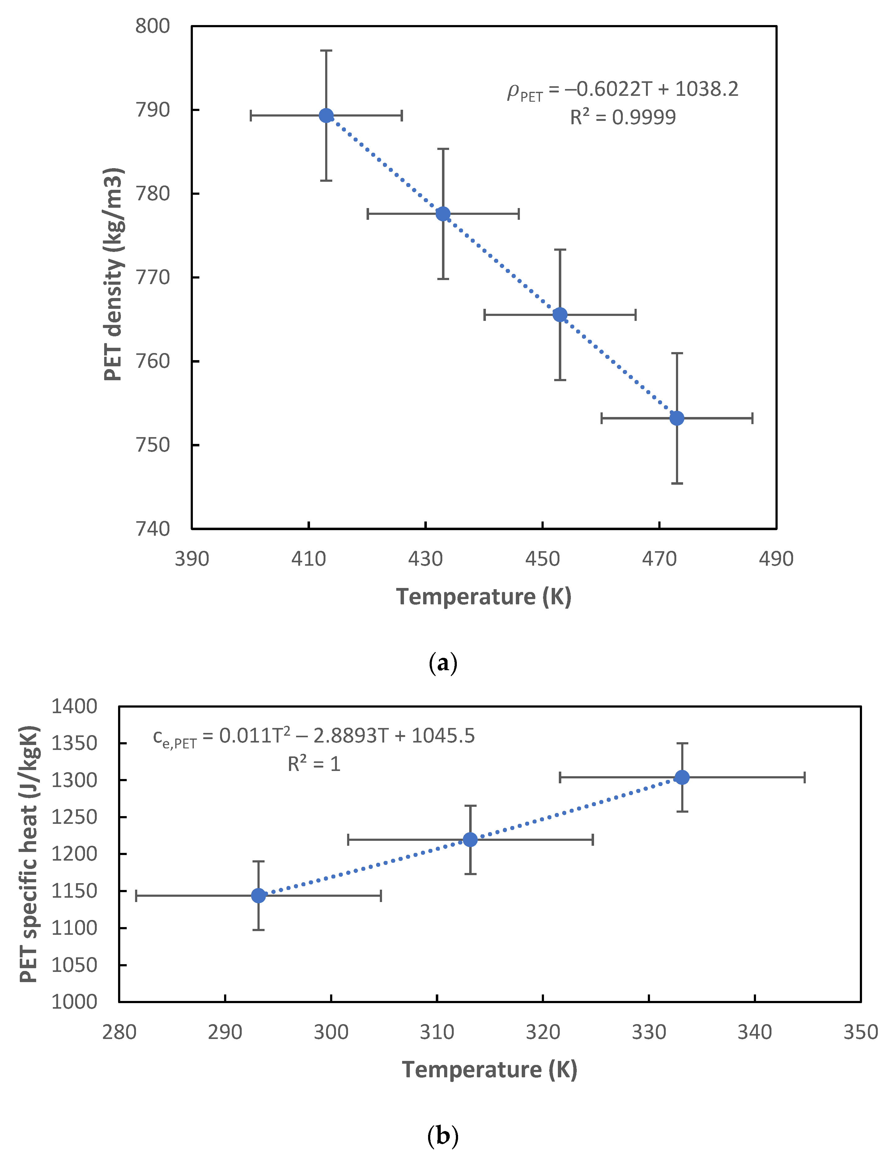
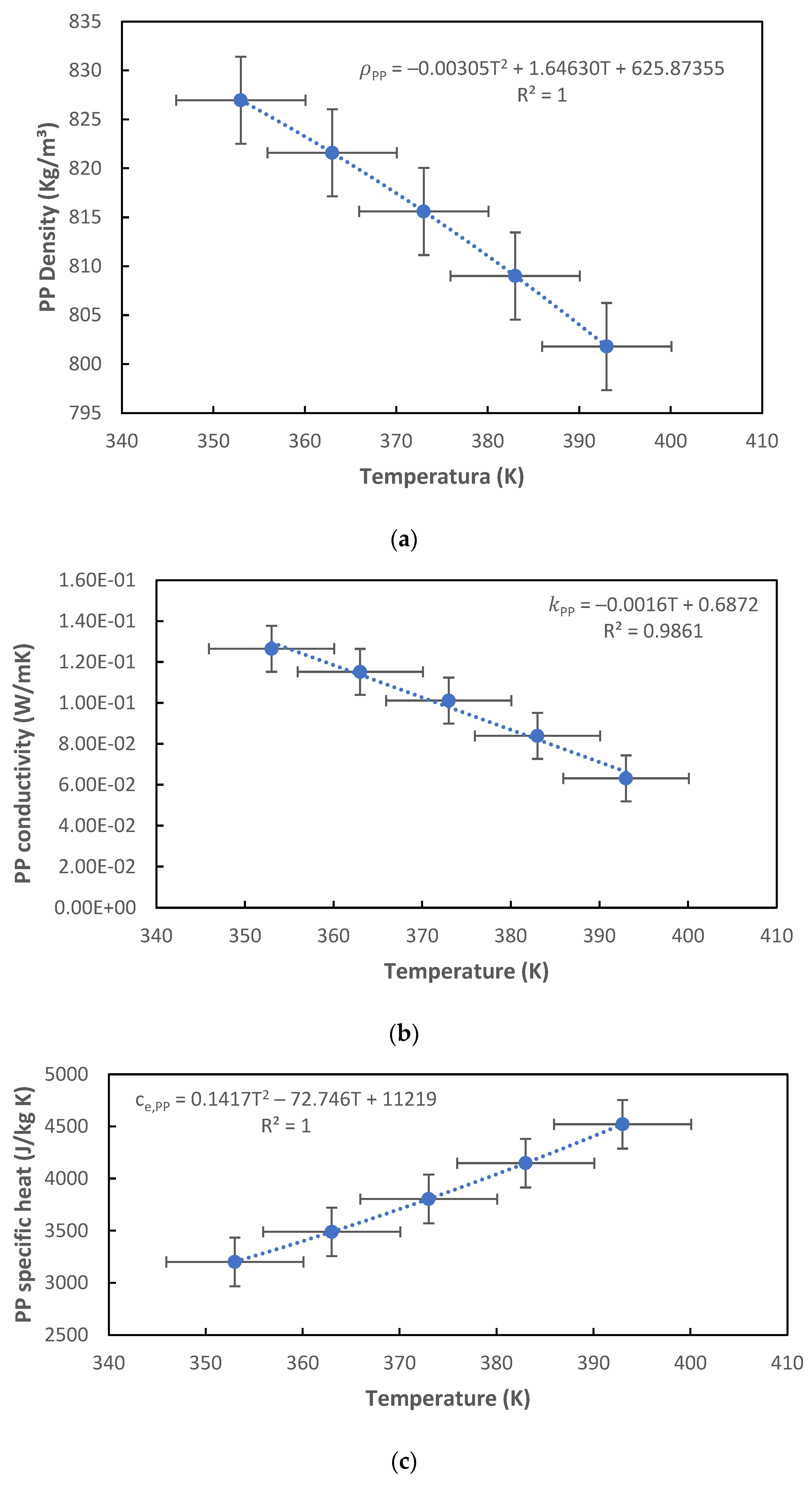
5.1. Material Properties Depending on Temperature

As mentioned above, we are going to focus, as an example, on the study of the heat transfer that takes place in a water bottle, considering that the value of the density, specific heat, and thermal conductivity of the materials depend on the temperature [10,40,41,42,43]. The materials recently used for water bottles are aluminium (Al319 in this case), polyethylene terephthalate (PET) and polypropylene (PP).
The following equations have been used to determine the density, thermal conductivity, and specific heat of the aluminium 319 (Al319) that will be the material of which our container is made:
ρ A l T = 2668.4118 0.3111 T   ( kg / m 3 )
k A l T = 76.64 + 0.2633 T 2 · 10 4 T 2   ( W / m K )
c e A l T = 747.3 + 0.2 T + 5 · 10 4 T 2   ( J / k g K )
The properties are represented graphically as follows, Figure 4:
The inside of the bottle will contain water, so it is also necessary to know the above-mentioned properties of water. The following equations have been used to determine the density, thermal conductivity and specific heat:
ρ W a t e r T = 0.0046 T 2 + 2.5216 T + 656.4   ( kg / m 3 )
k W a t e r T = 1 · 10 5 T 2 + 0.009 T 0.9864   ( W / m K )
c W a t e r T = 2 · 10 4 T 3 + 0.2026 T 2 69.268 T + 12010   ( J / k g K )
Properties are represented graphically as follows, Figure 5:
To determine the density and specific heat of PET which is the traditional material used in water bottles, the following equations have been used.
ρ P E T T = 0.6022 T + 1038.2   ( k g / m 3 )
c e P E T T = 0.011 T 2 2.8893 T + 1045.5   ( J / k g K )
The thermal conductivity of PET can be considered constant since, in the temperature ranges in which we are going to work, there are no significant differences in its value. The value of the thermal conductivity will be 0.2976 (W/mK).
Properties are represented graphically as follows, Figure 6:
To determine the density, specific heat and thermal conductivity of PP, the following equations have been used:
ρ P P T = 0.00305 T 2 + 1.6463 T + 625.87   ( kg / m 3 )
k P P T = 0,0016 T + 0.6872   ( W / m K )
c e P P T = 0.1417 T 2 72.746 T + 11,219   ( J / k g K )
Properties are represented graphically as follows, Figure 7:
As shown in the figures above, in many cases, the properties show wide variations in their value with temperature.

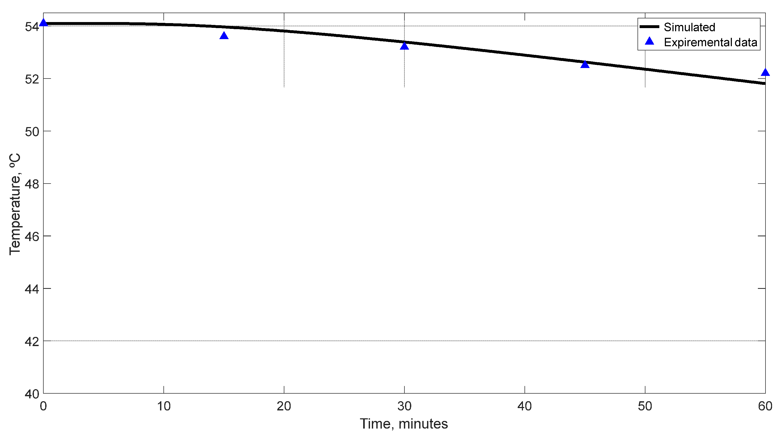
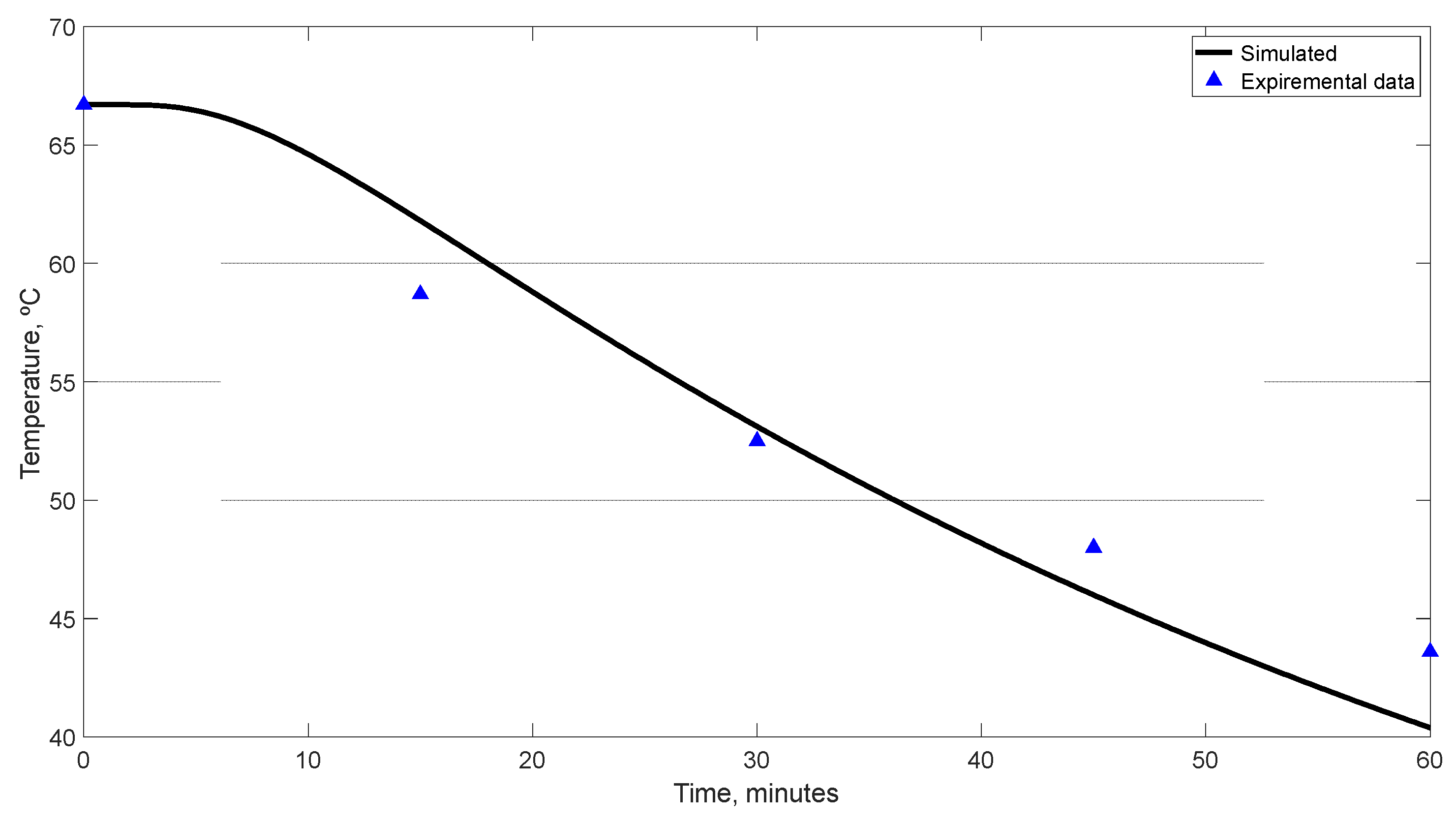
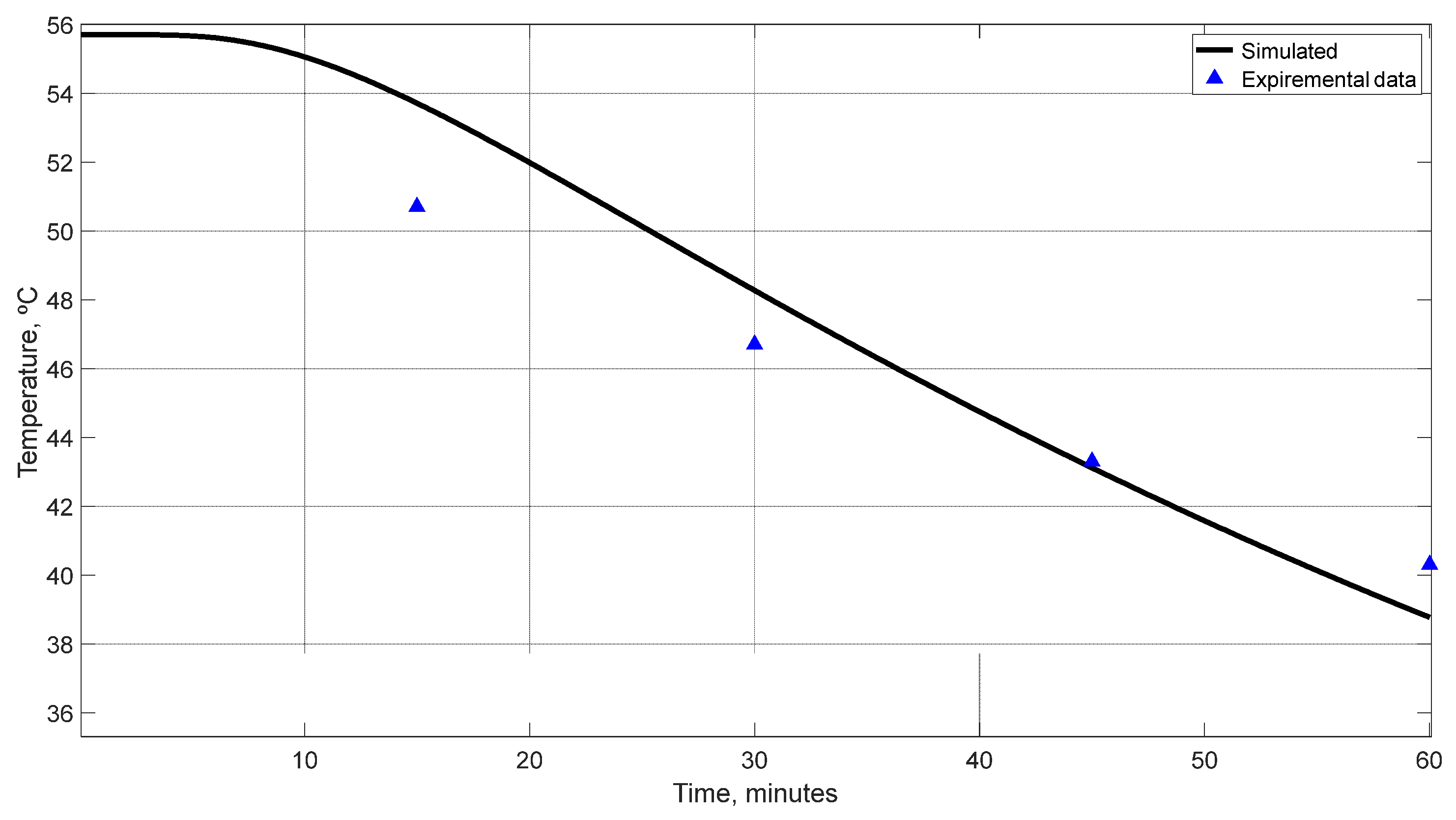
5.2. Model Validation

To validate both the mathematical model and the network model, a laboratory test was carried out with three cylindrical bottles of similar dimensions made with the materials indicated in the previous subsection, Table 1. It should be noted that the aluminium bottle was covered with a thin layer of insulating material, which in the network model has been implemented as a resistance. The experiment was carried out in a room that allowed the total absence of light without the influence of any type of radiation and with a constant room temperature during the entire test. Thus, the heat transfer was carried out mainly by conduction and convection. Therefore, the control of the input variables facilitates the validation of the proposed model. To measure the water and environmental temperatures, a thermometer with an error of ±0.1 °C was used, and the measurements were always taken in the central part of each of the cylindrical bottles. In order to compare these results with the proposed model, the properties that influence the problem (density, thermal conductivity, and specific heat) were introduced depending on the temperature at which the material was found. This relationship with temperature was obtained from the references mentioned above.
The experimental procedure consists of introducing water at a temperature higher than 50 °C in each of the bottles and exposing them to cooling conditions, mainly by convection, and without heating due to solar radiation. Temperature measurements were made at the midpoint of the vertical axis of each of the bottles and measured every 15 min until reaching a total time of one hour, Table 2. The ambient temperature at the beginning of the tests was 18.7 °C.
As stated above, the experimental tests were simulated by introducing the properties described above for each of the materials. Figure 8, Figure 9 and Figure 10 show the comparison between the results obtained in the simulation and those obtained experimentally. As can be seen, the trend obtained validates the proposed mathematical model, especially in the case of aluminium. In the cases of plastic materials, PP and PET, the deviation is greater due to the heterogeneity in the properties of these materials, as indicated in the previous section. However, in all cases, the evolution trend shown in the simulation is the same as that shown in the experimental test.

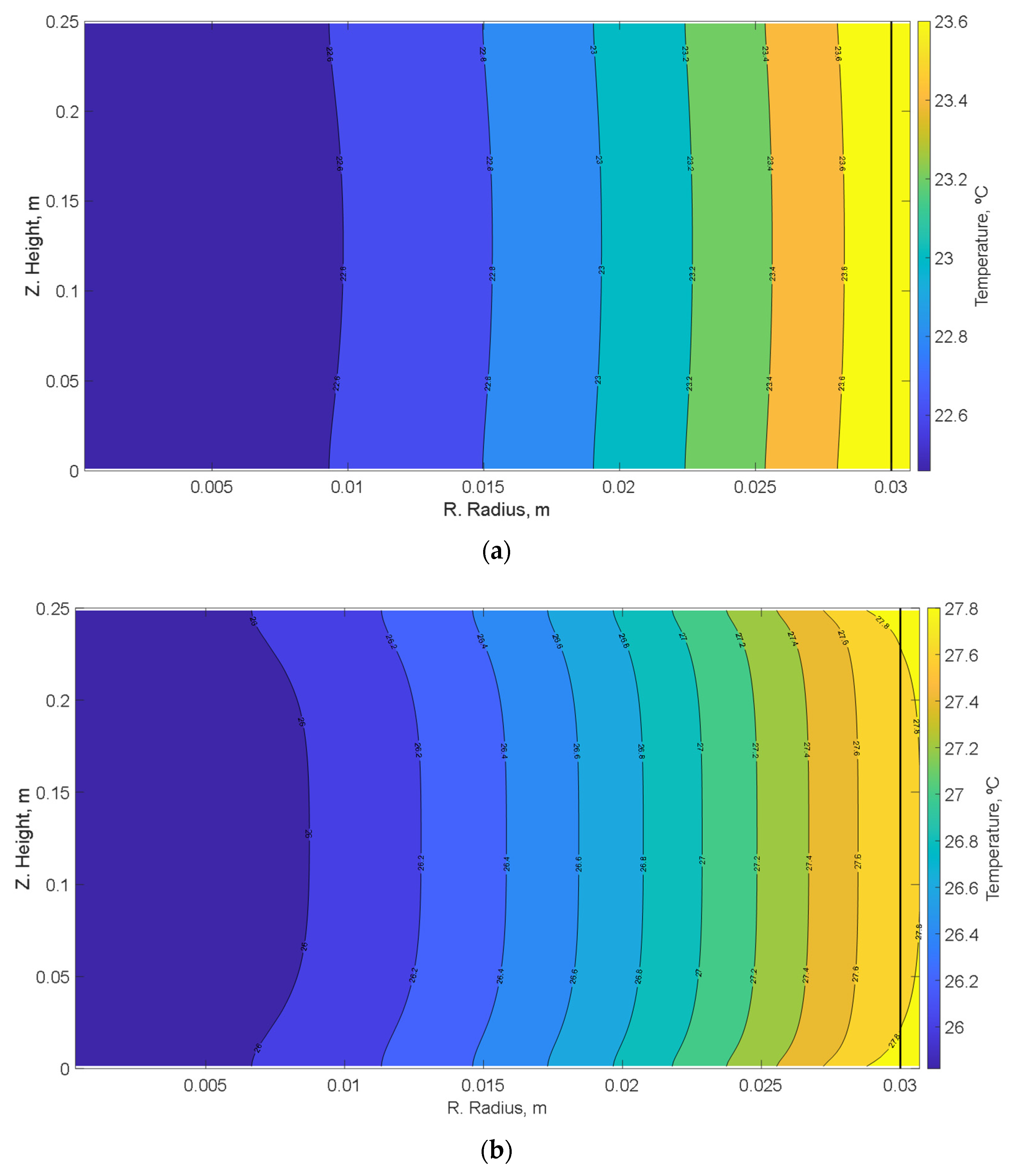
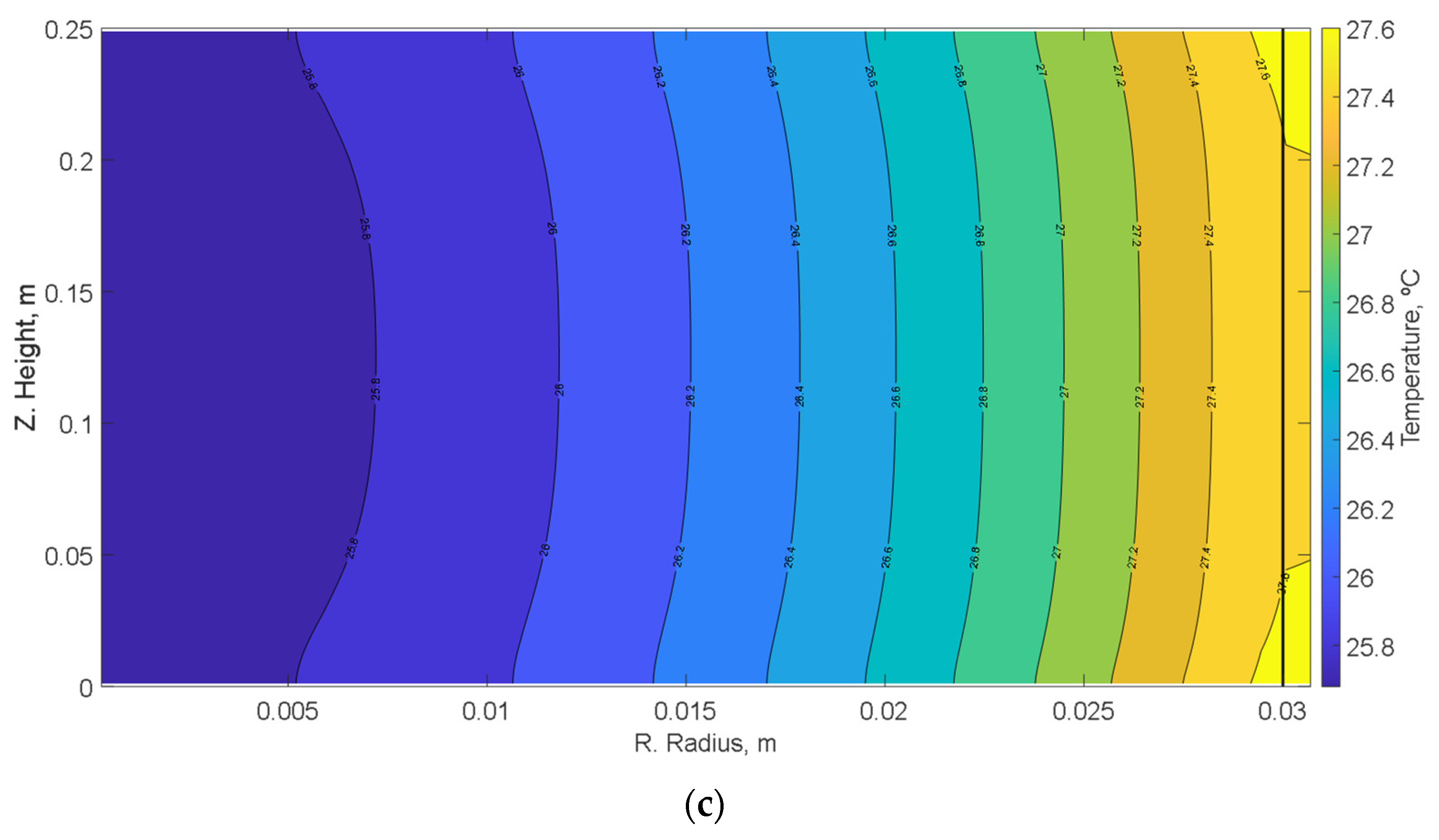
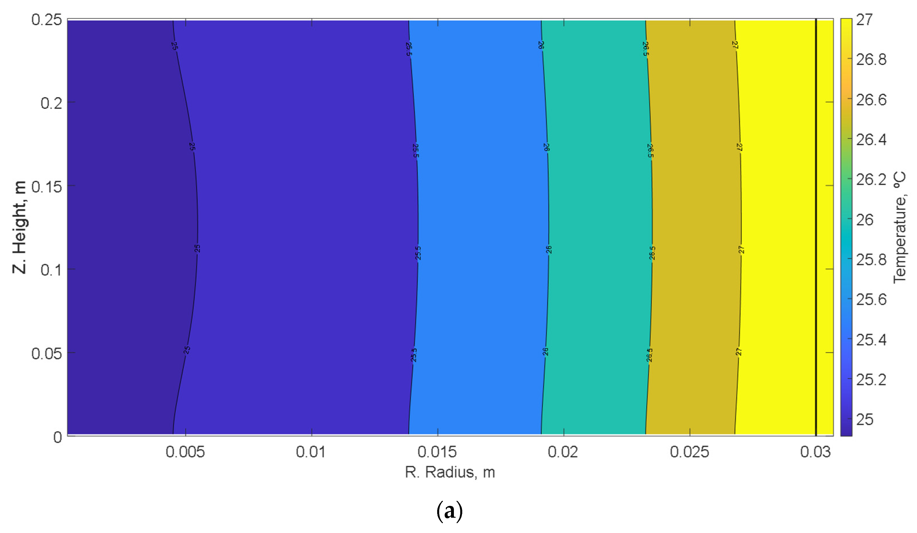
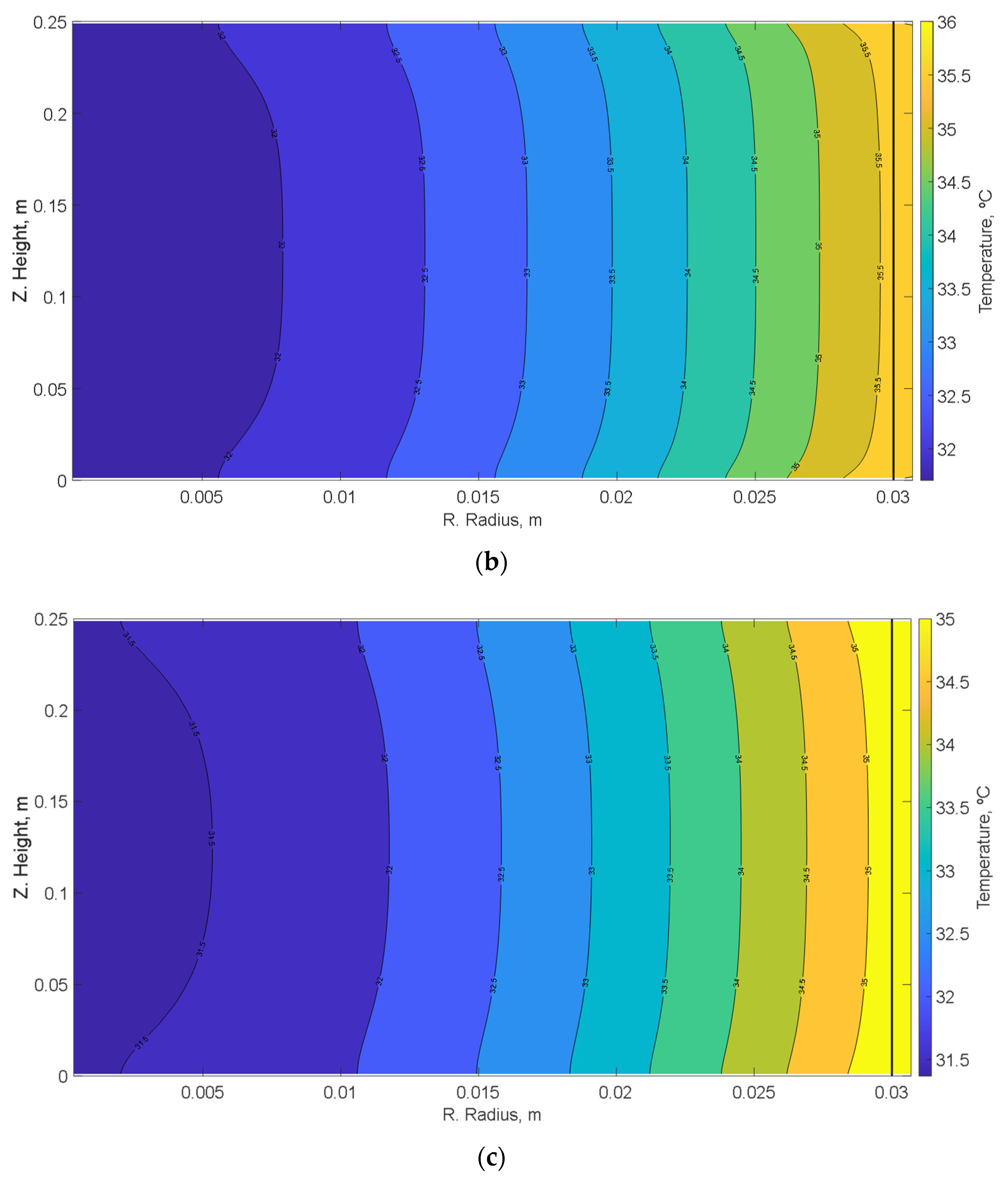
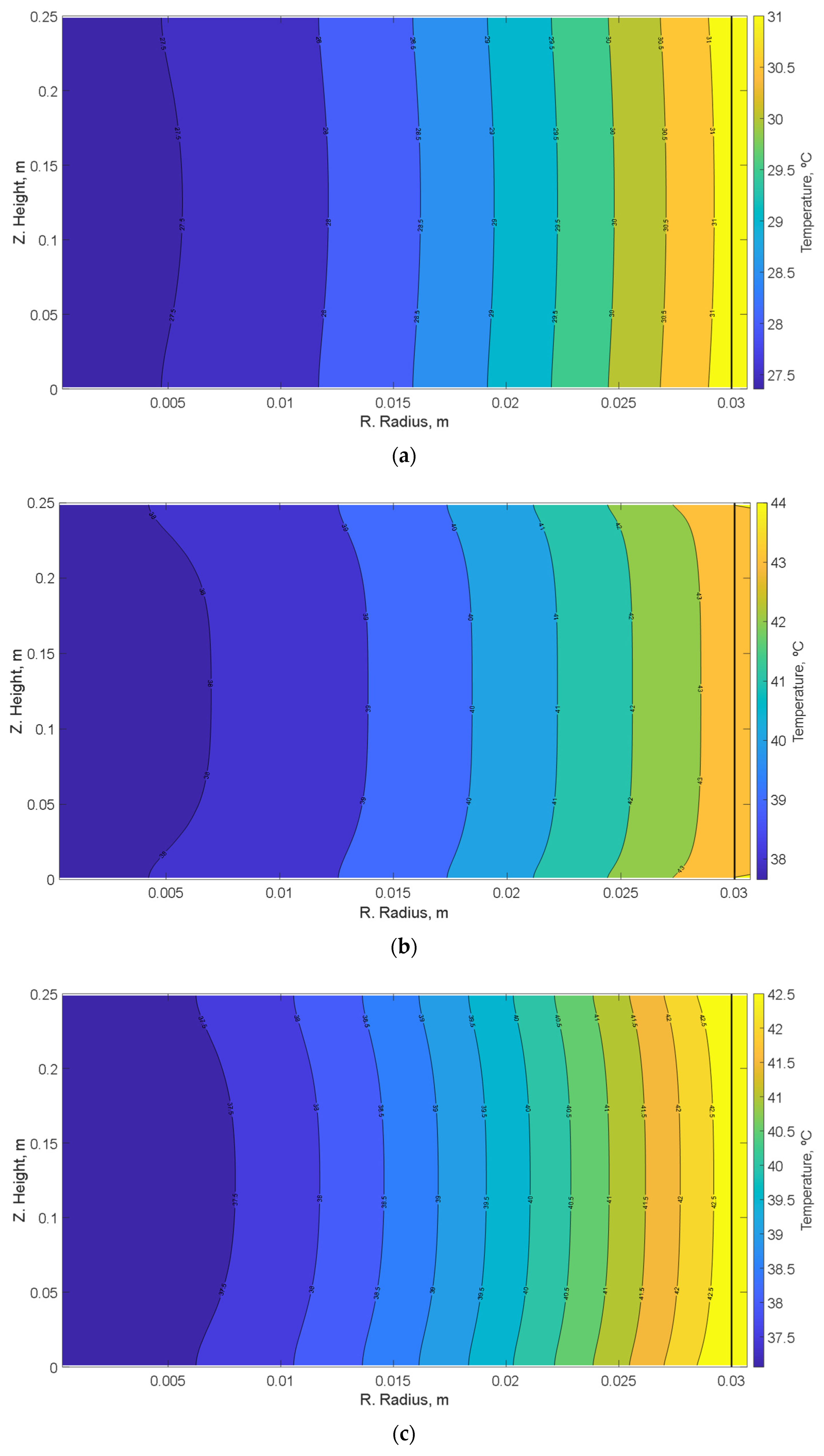
6. Results, Case Studies, and Conclusions

Once the mathematical model has been validated, we want to study the behaviour of these materials, used in commonly used water bottles, when exposed to summer temperatures, which in some areas of the Mediterranean can range between 30 and temperatures close to 50 °C in the shade. The foundation of this study is based on the migration of substances from plastic materials to water. Recent studies have determined that at a temperature of 40 °C, spring water in high-density polyethylene (HDPE) bottles contains 180 ng/L of nonylphenol, known for its endocrine-disrupting potential [28]. Other PET studies have found concentrations from 19 to 78 ng/L of this substance in mineral water from PET bottles [44]. Other investigations carried out on plastic water bottles have found migrations of compounds such as dimethyl phthalate (DMP), DEHP, and OP, among others, for PP and PET materials [27].
In this way, in order to compare the behaviour of the materials, it is assumed that the bottles will have the same dimensions, 25 cm in height, 3 cm in radius and 1 mm in thickness. In all cases, the initial temperature of both the water and the material, Al319, PP and PET, will be 20 °C, and they will be exposed to different ambient temperatures, Table 3. The heating of the material occurs mainly by convection since we have assumed that they are isolated from solar radiation. Thus, Figure 11, Figure 12 and Figure 13 show the temperature distribution for one hour for each of the materials and ambient temperatures. The black line on the right side of the image represents the boundary between the water and the bottle material. This point will be the reference point for comparisons between the materials studied, Table 3. In addition, the results for an ambient temperature of 60 °C have been added. As can be seen, the material that increases its temperature the least is Al319, presenting temperature differences of up to 12 °C with plastic materials for an ambient temperature of 50 °C, possibly because of the thin layer of insulation on the bottle. Plastic materials, PET and PP, present similar temperature values, being slightly lower in the case of PP. In both cases, we find temperatures close to ambient. It should be noted that the results obtained in this test depend on the materials used, and other aluminium alloys or variations in the composition of plastic materials could significantly change the result obtained. It is important to highlight that the behavior of the bottles validates the results obtained through the nondimensionalization technique, Equation (21). Finally, in all the distribution figures, the radial distribution of the problem in temperatures is clearly appreciated.
In conclusion, in this paper, a mathematical model capable of simulating cylindrical containers containing fluids whose properties are dependent on temperature has been fully developed. The simulation has been carried out using the Network Simulation Method, where the construction of the network model has been presented in detail. In addition, this has been validated with experimental tests carried out on three cylindrical containers made of aluminium, PET, and PP.
Moreover, the properties of materials whose value depends on temperature have been presented, highlighting the difficulty, in some cases, of obtaining experimental values as a function of temperature in the bibliography since it is common to take a constant value of these properties [10]. However, nowadays, more and more works are showing the dependence of these properties on temperature, making it necessary to develop mathematical models that include this dependence, thus improving the reliability of the simulations [10,11,12,13,14,15,16].
On the other hand, the nondimensionalization technique has also been applied, which allows us to obtain the weight of each of the variables on the problem, determining that the cooling or heating speed depends on the thermal diffusivity, as expected, and of the relationship between heat transfer coefficient and the material thermal conductivity, that is, the Nusselt number.
Finally, by way of illustration, a case has been studied where aluminium, PET, and PP mineral water bottles are exposed to summer environmental conditions, where temperatures close to 50 °C are reached. It should be noted that the best behaviour is presented by aluminium with a temperature difference of up to 12 °C with plastic materials, possibly because of the thin layer of insulation on the bottle. As a conclusion of the case study, the temperatures reached by the water in the summer season could imply migrations of different substances from plastic materials, PET and PP.

Author Contributions

Conceptualization, J.F.S.-P., M.F.-G. and F.d.C.; methodology, J.F.S.-P., M.F.-G., F.d.C. and M.C.; software, J.F.S.-P. and M.F.-G.; validation, J.F.S.-P., M.F.-G., F.d.C. and M.C.; formal analysis, J.F.S.-P., M.F.-G., F.d.C. and M.C.; writing—original draft preparation, J.F.S.-P., M.F.-G., F.d.C. and M.C.; writing—review and editing, J.F.S.-P., M.F.-G., F.d.C. and M.C. All authors have read and agreed to the published version of the manuscript.

Funding

This research received no external funding.

Informed Consent Statement

Not applicable.

Data Availability Statement

Data is contained within the article.

Conflicts of Interest

The authors declare no conflict of interest.

References

  1. Bejan, A. Convection Heat Transfer; John Wiley & Sons: Hoboken, NJ, USA, 1995; p. 623. [Google Scholar]
  2. Bejan, A.; Kraus, A. Heat Transfer Handbook; John Wiley & Sons: Hoboken, NJ, USA, 2003; Available online: https://books.google.com/books?hl=es&lr=&id=d4cgNG_IUq8C&oi=fnd&pg=PP11&ots=28zTda2t1B&sig=6yXJBvtqgJxIlD72No6ehnMMHYw (accessed on 2 January 2022).
  3. Jordan, J.L.; Casem, D.T.; Bradley, J.M.; Dwivedi, A.K.; Brown, E.N.; Jordan, C.W. Mechanical Properties of Low Density Polyethylene. J. Dyn. Behav. Mater. 2016, 2, 411–420. [Google Scholar] [CrossRef] [Green Version]
  4. Zenkour, A.M.; Abbas, I.A. A generalized thermoelasticity problem of an annular cylinder with temperature-dependent density and material properties. Int. J. Mech. Sci. 2014, 84, 54–60. [Google Scholar] [CrossRef]
  5. Ding, S.; Wu, C.P. Optimization of material composition to minimize the thermal stresses induced in FGM plates with temperature-dependent material properties. Int. J. Mech. Mater. Des. 2018, 14, 527–549. [Google Scholar] [CrossRef]
  6. Haopeng, S.; Kunkun, X.; Cunfa, G. Temperature, thermal flux and thermal stress distribution around an elliptic cavity with temperature-dependent material properties. Int. J. Solids Struct. 2021, 216, 136–144. [Google Scholar] [CrossRef]
  7. Demirbas, M.D. Thermal stress analysis of functionally graded plates with temperature-dependent material properties using theory of elasticity. Compos. B Eng. 2017, 131, 100–124. [Google Scholar] [CrossRef]
  8. Noda, N. Thermal stresses in materials with temperature-dependent properties. Appl. Mech. Rev. 1991, 44, 383–397. [Google Scholar] [CrossRef]
  9. del Cerro Velázquez, F.; Gómez-Lopera, S.A.; Alhama, F. A powerful and versatile educational software to simulate transient heat transfer processes in simple fins. Comput. Appl. Eng. Educ. 2008, 16, 72–82. [Google Scholar] [CrossRef]
  10. Mark, J.E. Physical Properties of Polymers Handbook, 2nd ed.; Springer Science+Business Media, LLC: Berlin/Heidelberg, Germany, 2007. [Google Scholar]
  11. Ozawa, S.; Morohoshi, K.; Hibiya, T. Influence of oxygen partial pressure on surface tension of molten type 304 and 316 stainless steels measured by oscillating droplet method using electromagnetic levitation. ISIJ Int. 2014, 54, 2097–2103. [Google Scholar] [CrossRef] [Green Version]
  12. Fukuyama, H.; Higashi, H.; Yamano, H. Thermophysical Properties of Molten Stainless Steel Containing 5 mass % B4C. Nucl. Technol. 2019, 205, 1154–1163. [Google Scholar] [CrossRef] [Green Version]
  13. Pichler, P.; Leitner, T.; Kaschnitz, E.; Rattenberger, J.; Pottlacher, G. Surface Tension and Thermal Conductivity of NIST SRM 1155a (AISI 316L Stainless Steel). Int. J. Thermophys. 2022, 43, 66. [Google Scholar] [CrossRef]
  14. Plebanski, T. Recommended Reference Materials for Realization of Physicochemical Properties. Pure Appl. Chem. 2007, 52, 2392–2404. [Google Scholar] [CrossRef] [Green Version]
  15. Daubert, T.E.; Danner, R.P. Physical and thermodynamic properties of pure chemicals: Data compilation. Choice Rev. Online 1990, 27, 3319. [Google Scholar] [CrossRef]
  16. Coker, A.K. Ludwig’s Applied Process Design for Chemical and Petrochemical Plants, 4th ed.; Gulf Professional Publishing: Houston, TX, USA, 2010; Volume 2. [Google Scholar] [CrossRef]
  17. Alhama, F.; Campo, A. Electric network representation of the unsteady cooling of a lumped body by nonlinear heat transfer modes. J. Heat Transfer. 2002, 124, 988–991. [Google Scholar] [CrossRef]
  18. Alhama, F.; González-Fernández, C.F. Network simulation method for solving phase-change heat transfer problems with variable thermal properties. Heat Mass Transfer/Waerme- und Stoffuebertragung 2002, 38, 327–335. [Google Scholar] [CrossRef]
  19. Sánchez-Pérez, J.F.; Marín, F.; Morales, J.L.; Cánovas, M.; Alhama, F. Modeling and simulation of different and representative engineering problems using network simulation method. PLoS ONE 2018, 13, e0193828. [Google Scholar] [CrossRef] [Green Version]
  20. Perez, J.F.S.; Conesa, M.; Alhama, I. Solving ordinary differential equations by electrical analogy: A multidisciplinary teaching tool. Eur. J. Phys. 2016, 37, 065703. [Google Scholar] [CrossRef]
  21. Sánchez-Pérez, J.F.; Alhama, I. Universal curves for the solution of chlorides penetration in reinforced concrete, water-saturated structures with bound chloride. Commun. Nonlinear. Sci. Numer. Simul. 2020, 84, 105201. [Google Scholar] [CrossRef]
  22. Sánchez-Pérez, J.F.; Alhama, F.; Moreno, J.A.; Cánovas, M. Study of main parameters affecting pitting corrosion in a basic medium using the network method. Results Phys. 2019, 12, 1015–1025. [Google Scholar] [CrossRef]
  23. García-Ros, G.; Alhama, I.; Morales, J.L. Numerical simulation of nonlinear consolidation problems by models based on the network method. Appl. Math. Model 2019, 69, 604–620. [Google Scholar] [CrossRef]
  24. Morales, N.G.; Sánchez-Pérez, J.F.; Nicolás, J.A.M.; Killinger, A. Modelling of alumina splat solidification on preheated steel substrate using the network simulation method. Mathematics 2020, 8, 1568. [Google Scholar] [CrossRef]
  25. Baranovskii, E.S. Optimal Boundary Control of the Boussinesq Approximation for Polymeric Fluids. J. Optim. Theory Appl. 2021, 189, 623–645. [Google Scholar] [CrossRef]
  26. Nigri, M.R.; Pedrosa-Filho, J.J.; Gama, R.M.S. An exact solution for the heat transfer process in infinite cylindrical fins with any temperature-dependent thermal conductivity. Therm. Sci. Eng. Prog. 2022, 32, 101333. [Google Scholar] [CrossRef]
  27. Guart, A.; Bono-Blay, F.; Borrell, A.; Lacorte, S. Effect of bottling and storage on the migration of plastic constituents in Spanish bottled waters. Food Chem. 2014, 156, 73–80. [Google Scholar] [CrossRef] [PubMed]
  28. Loyo-Rosales, J.E.; Rosales-Rivera, G.C.; Lynch, A.M.; Rice, C.P.; Torrents, A. Migration of Nonylphenol from Plastic Containers to Water and a Milk Surrogate. J. Agric. Food Chem. 2004, 52, 2016–2020. [Google Scholar] [CrossRef]
  29. Hao, L.; Xu, F.; Chen, Q.; Wei, M.; Chen, L.; Min, Y. A thermal-electrical analogy transient model of district heating pipelines for integrated analysis of thermal and power systems. Appl. Therm. Eng. 2018, 139, 213–221. [Google Scholar] [CrossRef]
  30. Kreith, F.; Manglik, R.M.; Bohn, M.S. Principles of Heat Transfer, SI Edition, 7th ed.; West Publishing Company: Eagan, MN, USA, 1999; Volume 2. [Google Scholar]
  31. Zheng, W.; Zhu, J.; Luo, Q. Distributed Dispatch of Integrated Electricity-Heat Systems with Variable Mass Flow. IEEE Trans Smart Grid 2022, 1. [Google Scholar] [CrossRef]
  32. Holger, V.; Atkinson, G.; Nenzi, P.; Warning, D. Software “NgSpice”. Available online: https://ngspice.sourceforge.io/index.html (accessed on 2 January 2022).
  33. Nagel, L.W. SPICE2: A Computer Program to Simulate Semiconductor Circuits; University of California: Berkeley, CA, USA, 1975. [Google Scholar]
  34. Gear, C.W. The automatic integration of ordinary differential equations. Commun. ACM 1971, 14, 176–179. [Google Scholar] [CrossRef]
  35. Nagel, L.W.; Pederson, D.O. SPICE (Simulation Program with Integrated Circuit Emphasis); EECS Department: Berkeley, CA, USA, 1973. [Google Scholar]
  36. Pérez, J.F.S.; Conesa, M.; Alhama, I.; Alhama, F.; Cánovas, M. Searching fundamental information in ordinary differential equations. Nondimensionalization technique. PLoS ONE 2017, 12, e0185477. [Google Scholar] [CrossRef] [Green Version]
  37. Sánchez-Pérez, J.F.; Conesa, M.; Alhama, I.; Cánovas, M. Study of Lotka–Volterra Biological or Chemical Oscillator Problem Using the Normalization Technique: Prediction of Time and Concentrations. Mathematics 2020, 8, 1324. [Google Scholar] [CrossRef]
  38. Conesa, M.; Pérez, J.F.S.; Alhama, I.; Alhama, F. On the nondimensionalization of coupled, non-linear ordinary differential equations. Nonlinear. Dyn. 2016, 84, 91–105. [Google Scholar] [CrossRef]
  39. Madrid, C.; Alhama, F. Análisis Dimensional Discriminado en Mecánica de Fluidos y Transferencia de Calor; Editorial Reverté: Barcelona, Spain, 2012. [Google Scholar]
  40. Valencia, J.J.; Quested, P.N. Thermophysical Properties. ASM Handb. Cast. 2008, 15, 468–481. [Google Scholar] [CrossRef]
  41. Mark, J.E. Physical Properties of Polymers Handbook. In Physical Properties of Polymers Handbook; Springer: New York, NY, USA, 2007. [Google Scholar] [CrossRef] [Green Version]
  42. Jagga, S.; Vanapalli, S. Cool-down time of a polypropylene vial quenched in liquid nitrogen. Int. Commun. Heat Mass. Transf. 2020, 118, 104821. [Google Scholar] [CrossRef]
  43. Kalaprasad, G.; Pradeep, P.; Mathew, G.; Pavithran, C.; Thomas, S. Thermal conductivity and thermal diffusivity analyses of low-density polyethylene composites reinforced with sisal, glass and intimately mixed sisal/glass fibres. Compos. Sci. Technol. 2000, 60, 2967–2977. [Google Scholar] [CrossRef]
  44. Toyo’oka, T.; Oshige, Y. Determination of alkylphenols in mineral water contained in PET bottles by liquid chromatography with coulometric detection. Anal. Sci. 2000, 16, 1070–1076. [Google Scholar] [CrossRef] [Green Version]
Figure 1. Cylindrical geometry.
Axioms 12 00335 g001
Figure 2. Volume element nomenclature.
Axioms 12 00335 g002
Figure 3. Network model of a volume element. (a) Temperature, (b) Density, (c) Thermal conductivity, (d) Specific heat capacity, and (e) Thermal diffusivity.
Axioms 12 00335 g003
Figure 4. Al 319 relation between material properties and temperature. (a) Density, (b) Thermal conductivity, and (c) Specific heat.
Axioms 12 00335 g004
Figure 5. Water relation between material properties and temperature. (a) Density, (b) Thermal conductivity, and (c) Specific heat.
Axioms 12 00335 g005
Figure 6. PET relation between material properties and temperature. (a) Density and (b) Specific heat.
Axioms 12 00335 g006
Figure 7. PP relation between material properties and temperature. (a) Density, (b) Thermal conductivity, and (c) Specific heat.
Axioms 12 00335 g007
Figure 8. Comparison between experimental and simulated data for the Al 319 temperature at the bottle centre.
Axioms 12 00335 g008
Figure 9. Comparison between experimental and simulated data for the PET temperature at the bottle centre.
Axioms 12 00335 g009
Figure 10. Comparison between experimental and simulated data for the PP temperature at the bottle centre.
Axioms 12 00335 g010
Figure 11. Distribution of temperatures for each of the materials at one hour and an ambient temperature of 30 °C. (a) Al319, (b) PET, and (c) PP.
Axioms 12 00335 g011aAxioms 12 00335 g011b
Figure 12. Distribution of temperatures for each of the materials at one hour and an ambient temperature of 40 °C. (a) Al319, (b) PET, and (c) PP.
Axioms 12 00335 g012aAxioms 12 00335 g012b
Figure 13. Distribution of temperatures for each of the materials at one hour and an ambient temperature of 50 °C. (a) Al319, (b) PET, and (c) PP.
Axioms 12 00335 g013
Table 1. Bottle dimensions.
MaterialAl319PETPP
Length (cm)20.522.023.0
Radio (cm)3.502.753.50
Thickness (mm)3.051.802.20
Table 2. Temperature measurements.
Temperature (°C)
Time (Minutes)Al319PETPP
054.166.755.7
1553.658.750.7
3053.252.546.7
4552.548.043.3
6052.243.640.3
Table 3. Temperature results of the simulations (°C).
Temperature at Reference Point (°C)
Room Temperature (°C)Al319PETPP
3023.7227.7727.58
4027.4335.5935.14
5031.1343.4842.69
6034.7251.4350.22
Disclaimer/Publisher’s Note: The statements, opinions and data contained in all publications are solely those of the individual author(s) and contributor(s) and not of MDPI and/or the editor(s). MDPI and/or the editor(s) disclaim responsibility for any injury to people or property resulting from any ideas, methods, instructions or products referred to in the content.

