
Homogeneity Test of Many-to-One Relative Risk Ratios in Unilateral and Bilateral Data with Multiple Groups


College of Mathematics and System Science, Xinjiang University, Urumqi 830046, China
*
Author to whom correspondence should be addressed.
Axioms 2023, 12(4), 333; https://doi.org/10.3390/axioms12040333
Submission received: 21 February 2023
/
Revised: 23 March 2023
/
Accepted: 26 March 2023
/
Published: 29 March 2023
(This article belongs to the Special Issue Fuzzy Logic and Application in Multi-Criteria Decision-Making (MCDM))
Abstract
:In medical clinical studies, we often encounter paired organs’ unilateral or bilateral data. For bilateral data, there exists an intraclass correlation between paired organs. Under an intraclass correlation model, this paper proposes asymptotic statistics for testing the equality of many-to-one relative risk ratios in combined unilateral and bilateral data. Furthermore, we calculate the explicit expressions of these statistics. Moreover, these procedures are adequate to solve the hypothesis problems of unilateral or bilateral data. Through comparison, the simulation results show that the score test has a robust empirical type-I error rate and sufficient power. We provide a clinical trial of acute otitis media to illustrate our proposed methods.
Keywords:
unilateral and bilateral data; Rosner’s model; likelihood ratio test; Wald-type test; score testMSC:
62F25; 91G70; 62P101. Introduction
Binary outcome data are widespread in medical applications. We often encounter the observation of paired organs (e.g., eyes, ears, and arms) in medical clinical studies. If only one of the patients’ paired organs is diseased, one organ’s response outcomes are not cured or cured; we call this unilateral data. Previous researchers have achieved outstanding achievements on statistical inferences about the unilateral data [1,2,3,4]. If both patients’ paired organs are diseased, the treatment responses of paired organs are none, one, and both cured; this is called bilateral data. Generally, the paired organs of patients may be correlated. Unlike the unilateral case, correlation should be considered in bilateral data to avoid biased results. For such correlated paired data, researchers have proposed many probabilistic models, including Rosner’s model [5], Dallal’s model [6], and Donner’s model [7]. Under the above models, various statistical methods have been proposed for testing the equality of proportions in bilateral data [8,9,10,11]. Among these models, Rosner’s model is the basis and has been widely studied [12,13,14].
In practice, we usually obtain both data types described above. Due to certain factors, some patients have only one eye studied, while others provide information on both eyes. For example, Mandel et al. [15] conducted a double-blind randomized clinical trial to treat acute otitis media (OME). In this trial, each child suffered either unilateral or bilateral tympanocentesis and was randomly assigned to receive treatment with Amoxicillin or Cefaclor. Under the same treatment method, we divided children into three groups by age. In the Amoxicillin treatment, 97 children of different ages were classified into three types: less than 2 years old, 2 to 5 years old, and 6 years old or older. After 14 days of treatment, Table 1 shows that each child underwent no, unilateral or bilateral OME, and was assigned into three groups according to age: <2, 2–5, and ≥6 years. Pei et al. [16] observed that the previous methods of studying unilateral or bilateral data are unsuitable for their combination. They proposed new asymptotical ways to test the equality of two proportions under such data. This topic is an emerging problem, and related research is less available [17,18,19,20]. Therefore, studying unilateral and bilateral data under Rosner’s model is imperative.
To compare the treatment of Amoxicillin in Table 1, the common measures are risk difference (RD), relative risk ratio (RR), and odds ratio (OR). The RD is an essential and straightforward measure that reflects the underlying risk without treatment and the risk reduction associated with treatment. The relative risk of a treatment is the ratio of risks between the treatment and control groups. It is generally more meaningful to use relative effect measures for summarizing the evidence and absolute measures. The odds ratio aims to look at associations rather than differences. Please note that RR and OR are related; this paper compares the relative risk ratios under Rosner’s model.
Multiple groups can often occur in many different treatments or over time in medical trials [21]. It is natural to compare several treatment groups with a control group. Mou and Li [22] considered a homogeneity test of risk differences on many-to-one bilateral data in a study. Schaarschmidt et al. [23] studied asymptotic simultaneous confidence intervals (SCIs) for many-to-one comparisons on binary proportion. Yang et al. [24] proposed asymptotic SCI construction for many-to-one comparisons of proportion differences adjusting for multiplicity and correlation. To date, relatively few papers have studied unilateral and bilateral data. Most research on unilateral or bilateral data mainly focuses on homogeneity testing for risk differences in stratified data, and on the study of equality of multiple groups of proportions. When the cure rates are low, and the difference between groups is slight, using the relative risk ratio to judge is more appropriate. There is insufficient research into statistical inference on many-to-one procedures of combined unilateral and bilateral data. Under Rosner’s model, the paper aims to study homogeneity tests of many-to-one relative risk ratios in unilateral and bilateral data. The hypothesis proposed by Ma et al. [17] is a particular case of this type. Moreover, the method proposed in this paper can also be applied to unilateral or bilateral data, and the corresponding test statistics are given. We arrange the rest of the work as follows. In Section 2, we introduce the data structure and Rosner’s model, and estimate the unknown parameters by algorithms. Section 3 constructs the likelihood ratio, score, and Wald-type statistics. In Section 4, through Monte Carlo simulations, we compare the performance of these test statistics in terms of the empirical type-I error rates and power. We provide a real example to illustrate our proposed method in Section 5 and conclude in Section 6.
2. Data Structure and Probability Distribution
In an ophthalmologic study, let be the number of patients with l response(s) for bilateral data. For unilateral data, let be the number of patients with l response in the ith group for . Table 2 shows the combined unilateral and bilateral data.
Let be the total number of patients with bilateral data in the ith group, and be the total number of patients with exactly response(s). For the unilateral case, is the total number of patients with binary data in the ith group, and is the total number of patients with response. We have
For the bilateral data, let be a random variable representing the number of patients with l response in the ith group, which has a trinomial distribution. In addition, is the corresponding probability. Define , , and . Then, the probability density of is
for . For the unilateral data, let be a random variable that represents the number of patients with l response in the ith group and follows a binomial distribution, and be the corresponding probability. We denote , , and . Then, the probability density of is
for .
Suppose in bilateral data if the kth eye of the jth individual is cured in the ith group and 0 otherwise. Define if the eye of the jth patient has a response in the ith group, and 0 otherwise for the unilateral patients. Under Rosner’s model, we propose a probability model of unilateral and bilateral data as
where R is a constant. If , the two organs of a patient are completely independent. They are completely dependent when .
From the probabilities of Equation (1), it is easy to derive , , , and for . Since and are independent random variables, the likelihood function is expressed by
where . Thus, we have the log-likelihood as
where is a constant.
Denote and . We aim to test whether the many-to-one relative risk ratios are identical and give the hypotheses as
Let and be the global maximum likelihood estimators (MLEs) of unknown parameters and R, respectively. Global MLEs are the solutions to the equations
where
Denote and . We simplify the first equation of (2) as the following 4th-order polynomial equations
where
The th update of R is obtained by the Newton–Raphson algorithm
where
Remark 1.
In the above algorithm, if , the global MLEs of and R correspond to the results of bilateral data in Ma et al. [14]. If , it is easy to obtain the global MLEs in unilateral data.
Suppose that under , the log-likelihood is rewritten by
where
Let , and be the constrained MLEs of , and R under the null hypothesis . We calculate the constrained MLEs of and R from
However, there is no close solution for Equation (3) when (see Appendix A.1). Given initial values , and , the Fisher scoring algorithm is introduced to obtain the th updates of and R as follows
where is a Fisher information matrix (see Appendix A.1), and
Remark 2.
Under , if , we can obtain the constrained MLEs of Rosner’s model through Equation (4) in bilateral data. If , the constrained MLEs of and δ are directly given by
3. Asymptotic Methods
This section uses the likelihood ratio, score, and Wald-type test for unilateral and bilateral data. Especially for bilateral or unilateral data, we provide three tests when and , respectively.
3.1. Likelihood Ratio Test
The likelihood ratio (LR) test can be given by
where
Under , the likelihood ratio test is asymptotically distributed as a chi-square distribution with a degree of freedom.
Remark 3.
If , the likelihood ratio test in the bilateral data can be calculated by
If , we simplify the likelihood ratio test of the unilateral data as
3.2. Score Test
Please note that is equivalent to . Denote , , and . The score statistic is expressed by
where is a Fisher information matrix (see Appendix A.2 for more information). Let
where
After calculation, the inverse matrix of can be obtained by
where
and the inverse matrix of is given by
Then
where
The score statistic can be simplified as
Under , the score test is asymptotically distributed as a chi-square distribution with a degree of freedom.
Remark 4.
For bilateral data, we can obtain the score test through the Equation (5) and . Suppose that , , and is a Fisher information matrix, where . The score test in unilateral data can be simplified as
3.3. Wald-Type Test
Let be the global MLEs of . The null hypothesis is equivalent to , where
Then, the Wald-type test statistic can be expressed as
where is the information matrix (see Appendix A.2 for more information), and can be derived as
Denote a matrix , and its element . It is convenient to express elements of the inverse matrix by a lower triangular matrix , i.e., , where and
Obviously, , where and its elements can be derived as follows
Thus, . The Wald-type statistic can be written as:
The Wald-type test is asymptotically distributed as a chi-square distribution with a degree of freedom under .
4. Monte Carlo Simulation Studies
In this section, we compare the performance of the statistics for the homogeneity test of risk ratios. In addition, we selected two evaluation indexes of type-I error rates (TIEs) and power. The fitting results of the homogeneity test are calculated when the significance level . The TIE is the probability of rejecting the null hypothesis when it is true. Each parameter set is performed 10,000 times based on the null hypothesis. The empirical TIEs is calculated as the number rejecting the null hypothesis divided by 10,000 at a significance level . According to Tang et al. [12], a test is liberal if the empirical TIEs is larger than 0.06, conservative if the empirical TIE rate is less than 0.04, and robust otherwise at the significance level .
First, we investigate the performance of TIEs under different parameter settings. Take the sample sizes , . Let for balanced designs and for unbalanced designs. Take , , and under the hypothesis . Then, we calculate the empirical TIEs of all proposed test statistics. For each scenario, 10,000 replicates are randomly generated under the null hypothesis .
Table 3, Table 4 and Table 5 show the empirical TIEs based on three statistics under all configurations for and 5, respectively. The left side of the table shows the balanced design results. We provide the unbalanced design results on the right of each table. Let , is equivalent to . This situation can be seen as the proportional homogeneity test proposed by Ma and Wang [17]. In Table 3, the likelihood ratio and score tests are robust for the balanced design and small sample size, while the Wald-type statistic is liberal. The Wald-type test tends to be robust when the sample size becomes larger. In the unbalanced design, let , the Wald-type statistic is liberal when and . Take , and the Wald-type test performs better. The result of the Wald-type statistic becomes more robust when the total sample sizes increase. Table 4 displays that the Wald-type test is more liberal for the unbalanced design. The likelihood ratio and score tests are more robust than the Wald-type tests for the balanced design, especially for a small sample size. In Table 5, the Wald-type test is worse for small sample sizes in unbalanced scenarios, similar to balanced ones.
In Table 3, Table 4 and Table 5, the score test and likelihood ratio test are more robust than Wald-type test in terms of the TIEs. The Wald-type statistic is liberal in small sample scenarios and becomes more liberal as the number of groups increases. There is no significant difference in the performance of the three statistics when the total sample sizes of the balanced and unbalanced groups are the same. As the values of m or n increase, we can observe that the Wald-type statistic tends to be robust. The TIEs of all three tests grow closer if the sample size increases.
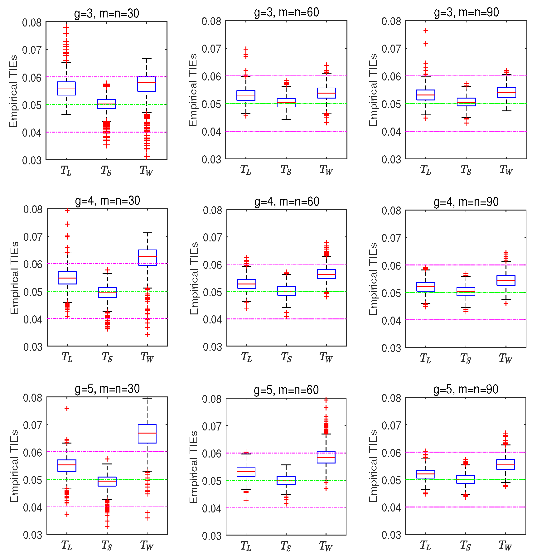
The above results are obtained for given multiple parameter values. In practice, there are more possibilities for parameter values. To further compare these test statistics, we randomly choose 1000 sets of parameters according to the constrained ranges of parameters for and under . A total of 10,000 replicates are randomly generated for each configuration to calculate the type-I error rates. Figure 1 shows the box plots of the empirical TIEs. The results display that the three statistics become more robust under the same number of groups as the sample size increases. As the number of groups grows, the Wald-type test becomes more liberal while the likelihood ratio and score tests become more robust. Overall, the score test is more robust in the sense that the TIE of it is close to the significant level regardless of sample size and the number of groups.
Next, we compare and summarize the performance of proposed test statistics in terms of power under different parameter settings. To be specific, we consider the balanced and unbalanced settings, respectively. In addition, we also take the same parameter as we do for empirical type-I error rates. Under the hypothesis , the parameter settings satisfy: for . Similarly, we randomly select 10,000 replicates from the alternative hypothesis for each parameter setting and calculate the empirical power by the number of rejections of the alternative hypothesis divided by 10,000. The simulated results are presented in Table 6 and Table 7, respectively. At the same number of groups, when we fix parameter R, the empirical powers will become larger as increases. However, given a fixed parameter , the empirical powers do not change much as R increases. In Table 7, the powers obtained with sample size of are greater than that obtained with . The results show that these powers of the three test statistics are very close under the same parameter settings. The empirical power will increase with the sample size or the number of groups.
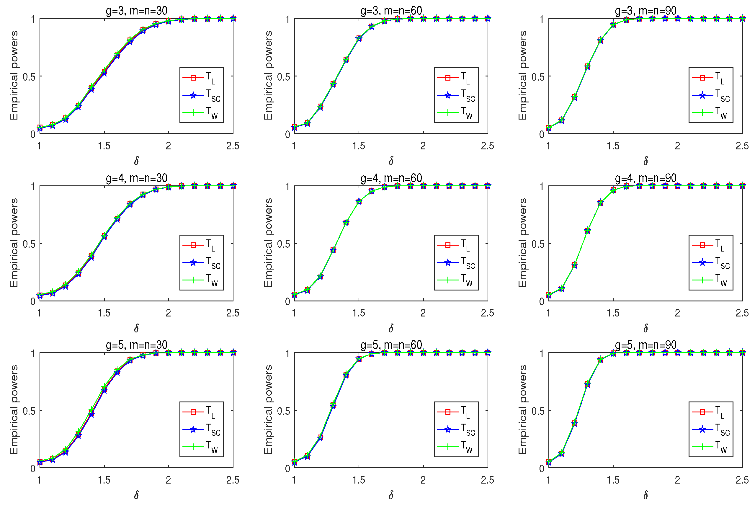
We further study the power of three statistics changes as the given parameters change. Under hypothesis , let , and for . Figure 2 reveals the empirical powers of three tests for given parameters . The performances of the three statistics are close in terms of powers. When is around 1, the resulting power is around 0.05. This is because the difference between the null and alternative hypotheses is small. The increasing leads to a significant power increase. The powers increase in the same number of groups as the sample size increases. The three statistics have good power performance when the number of groups increases.
According to the simulation results, the score statistic and LR test have satisfactory results in the TIEs. However, the score statistics are more robust than the other two for small sample-size scenarios. The powers of the three tests are very close. Thus, we recommend it for the homogeneity test about a many-to-one comparison of relative risk ratios.
5. A Real Example
In this section, we review the double-blinded randomized clinical trial of treating acute otitis media (OME) from Mandel et al. [15] to illustrate the proposed methods. In Table 1, and in the first group; for the second group, and ; and in the third group. Under Rosner’s model, an interesting test is whether there is a significant difference in many-to-one risk ratios. Thus, give the hypotheses as .
Let , then we use the formula in this article to obtain global MLEs and constrained MLEs. Global and constrained MLEs are given in Table 8. The results show a correlation between paired organs. The estimated relative risk ratios under is 0.6709, and global relative risk ratios can be calculated as in Table 9. The values of and are 5.3330, 3.8502, and 7.4055. At significance level , the values are bigger than the 95 percentile of the chi-square distribution with one degree of freedom, and p values of statistics are less than 0.05. Therefore, it provides stronger evidence to reject the null hypothesis . It means that there were significant differences in relative risk ratios between groups. We can find that if is less than 1, then children who were less than two years old had the highest cure rates in Amoxicillin-treated. Mandel et al. [15] find that children less than 2 years old had more OME. This is consistent with our results.
6. Conclusions
This paper introduces three statistics for testing the homogeneity of many-to-one relative risk ratios for bilateral and unilateral data under Rosner’s model. Then, we use a fourth-order polynomial and the Newton–Raphson algorithm to estimate the global maximum likelihood estimate. In addition, we obtain constrained MLEs under through the Fisher scoring method. Three statistics are proposed in bilateral and unilateral data. Moreover, we also offer global MLEs, constrained MLEs, and three statistics for unilateral and bilateral data, respectively. The Monte Carlo simulation was carried out with different parameter settings.
Based on the simulation results, the score test is more robust than the likelihood ratio and the Wald-type test regarding the TIEs and has sufficient power. The powers of the proposed three tests grow closer as the sample size becomes more significant. By comparison, the Wald-type test is better than the score test and the likelihood ratio test in terms of power. However, the Wald-type test has liberal type-I error rates under a small sample size. The results of the Wald-type test behave worse, especially when the number of groups is more extensive and the sample size is small. The score test performs well regardless of the number of groups and sample size. The score test is recommended for unilateral and bilateral data for the above reasons.
In future work, we will focus on other statistical problems of the many-to-one relative risk ratios for unilateral and bilateral data, such as confidence intervals.
Author Contributions
Methodology, Y.L.; software, Y.L.; writing—original draft preparation, Y.L.; writing—review and editing, Z.L. and K.M.; supervision, Z.L.; funding acquisition, Z.L. All authors have read and agreed to the published version of the manuscript.
Funding
This research was supported by the National Natural Science Foundation of China (Grant No: 12061070) and the Science and Technology Department of Xinjiang Uygur Autonomous Region (Grant No: 2021D01E13).
Data Availability Statement
Clinical data referred to are from Mandel et al. [15].
Conflicts of Interest
The authors declare no conflict of interest.
Abbreviations
The following abbreviations are used in this manuscript:
| RD | risk difference | RR | risk ratio |
| OR | odds ratio | SCIs | simultaneous confidence intervals |
| MLEs | maximum likelihood estimators | TIEs | type-I error rates |
| likelihood ratio statistic | score statistic | ||
| Wald-type statistic |
Appendix A
Appendix A.1. Information Matrix I1
The first-order differential equations of under null hypothesis are
The second-order differential equations of under null hypothesis are
Thus, we have
where
Appendix A.2. Information Matrix I2
Differentiating and with respect to and R yield
Therefore, we have
for .
Under the null hypothesis , the information matrix can be derived as
Appendix A.3. Information Matrix I3 and
The information matrix can be expressed as
and the elements of can be derived as follows
References
- Gart, J.J. The comparison of proportions: A review of significance tests, confidence intervals and adjustments for stratification. Rev. Int. Stat. Inst. 1971, 39, 148–169. [Google Scholar] [CrossRef]
- Gart, J.J. Approximate tests and interval estimation of the common relative risk in the combination of 2 × 2 tables. Biometrika 1985, 72, 673–677. [Google Scholar]
- Casagrande, J.T.; Pike, M.C.; Smith, P.G. An improved approximate formula for calculating sample sizes for comparing two binomial distributions. Biometrics 1978, 34, 483–486. [Google Scholar] [CrossRef] [PubMed]
- Storer, B.E.; Kim, C. Exact properties of some exact test statistics for comparing two binomial proportions. Publ. Am. Stat. Assoc. 1990, 85, 146–155. [Google Scholar] [CrossRef]
- Rosner, B. Statistical methods in ophthalmology: An adjustment for the intraclass correlation between eyes. Biometrics 1982, 38, 105–114. [Google Scholar] [CrossRef] [PubMed]
- Dallal, G.E. Paired bernoulli trials. Biometrics 1988, 44, 253–257. [Google Scholar] [CrossRef]
- Donner, A. Statistical methods in ophthalmology: An adjusted chi-square approach. Biometrics 1989, 45, 605–611. [Google Scholar] [CrossRef]
- Pei, Y.; Tian, G.L.; Tang, M.L. Testing homogeneity of proportion ratios for stratified correlated bilateral data in two-arm randomized clinical trials. Stat. Med. 2014, 33, 4370–4386. [Google Scholar] [CrossRef]
- Zhuang, T.; Tian, G.L.; Ma, C.X. Homogeneity test of ratio of two proportions in stratified bilateral data. Stat. Biopharm. Res. 2019, 11, 200–209. [Google Scholar] [CrossRef]
- Sun, S.M.; Li, Z.M.; Ai, M.Y.; Jiang, H.J. Risk difference tests for stratified binary data under Dallal’s model. Stat. Methods Med. Res. 2022, 31, 1135–1156. [Google Scholar] [CrossRef]
- Chen, Y.F.; Li, Z.M.; Ma, C.X. Further study on testing the equality of response rates under Dallal’s model. Stat. Its Interface 2022, 15, 115–126. [Google Scholar] [CrossRef]
- Tang, M.L.; Tang, N.S.; Rosner, B. Statistical inference for correlated data in ophthalmologic studies. Stat. Med. 2006, 25, 2771–2783. [Google Scholar] [CrossRef] [PubMed]
- Tang, N.S.; Tang, M.L.; Qiu, S.F. Testing the equality of proportions for correlated otolaryngologic data. Comput. Stat. Data Anal. 2008, 52, 3719–3729. [Google Scholar] [CrossRef]
- Ma, C.X.; Shan, G.; Liu, S. Homogeneity test for correlated binary data. PLoS ONE 2015, 10, e0124337. [Google Scholar] [CrossRef] [PubMed]
- Mandel, E.M.; Bluestone, C.D.; Rockette, H.E.; Blatter, M.M.; Reisinger, K.S.; Wucher, F.P.; Harper, J. Duration of effusion after antibiotic treatment for acute otitis media: Comparison of cefaclor and amoxicillin. Pediatr. Infect. Dis. 1982, 1, 310–316. [Google Scholar] [CrossRef] [PubMed]
- Pei, Y.B.; Tang, M.L.; Guo, J.H. Testing the equality of two proportions for combined unilateral and bilateral data. Commun.-Stat.-Simul. Comput. 2008, 37, 1–15. [Google Scholar] [CrossRef]
- Ma, C.X.; Wang, K.J. Testing the equality of proportions for combined unilateral and bilateral data. arXiv 2020, arXiv:2010.03501. [Google Scholar]
- Ma, C.X.; Wang, H. Testing the equality of proportions for combined unilateral and bilateral data under equal intraclass correlation model. Stat. Biopharm. Res. 2022. [Google Scholar] [CrossRef]
- Sun, S.M.; Li, Z.M.; Jiang, H.J. Homogeneity test and sample size of risk difference for stratified unilateral and bilateral data. Commun.-Stat.-Simul. Comput. 2022. [Google Scholar] [CrossRef]
- Li, Z.M.; Ma, C.X.; Mou, K.Y. Testing the common risk difference of proportions for stratified uni-and bilateral correlated data. Stat. Neerl. 2023. [Google Scholar] [CrossRef]
- Kropf, S.; Hothorn, L.A.; Lauter, J. Multivariate many-to-one procedures with applications to preclinical trials. Drug Inf. J. 1997, 31, 433–447. [Google Scholar] [CrossRef]
- Mou, K.Y.; Li, Z.M. Homogeneity test of many-to-one risk differences for correlated binary data under optimal algorithms. Complexity 2021, 2021, 6685951. [Google Scholar] [CrossRef]
- Schaarschmidt, F.; Biesheuvel, E.; Hothorn, L.A. Asymptotic simultaneous confidence intervals for many-to-one comparisons of binary proportions in randomized clinical trials. J. Biopharm. Stat. 2009, 19, 292–310. [Google Scholar] [CrossRef] [PubMed]
- Yang, Z.; Tian, G.L.; Liu, X.; Ma, C.X. Simultaneous confidence interval construction for many-to-one comparisons of proportion differences based on correlated paired data. J. Appl. Stat. 2021, 48, 1442–1456. [Google Scholar] [CrossRef] [PubMed]
Figure 1.
Empirical TIEs of tests.

Figure 2.
Empirical powers of tests.


Table 1.
OME status of Amoxicillin treatment.
| Responses | Age Group (Unit: yrs) | ||
|---|---|---|---|
| <2 | 2–5 | ≥6 | |
| 0 | 2 | 5 | 6 |
| 1 | 2 | 1 | 0 |
| 2 | 11 | 3 | 1 |
| Total | 15 | 9 | 7 |
| 0 | 2 | 14 | 11 |
| 1 | 10 | 22 | 7 |
| Total | 12 | 36 | 18 |
Note: response 0—no OME, response 1—unilateral OME, and response 2—bilateral OME.
Table 2.
The unilateral and bilateral data in g groups.
| Response | Group (i) | Total | |||
|---|---|---|---|---|---|
| 1 | 2 | … | g | ||
| 0 | … | ||||
| 1 | … | ||||
| 2 | … | ||||
| Total | … | ||||
| 0 | … | ||||
| 1 | … | ||||
| Total | … | ||||
Table 3.
The empirical TIEs (%) of tests under ().
| R | Balance | Unbalance | |||||||||||
|---|---|---|---|---|---|---|---|---|---|---|---|---|---|
| 1.1 | 0.3 | 5.47 | 5.01 | 5.62 | 5.65 | 4.97 | 5.73 | 5.58 | 5.06 | 5.53 | 5.59 | 5.12 | 5.51 |
| 0.4 | 5.54 | 5.16 | 5.85 | 5.50 | 5.15 | 6.04 | 5.29 | 4.96 | 5.48 | 5.25 | 4.90 | 5.62 | |
| 0.5 | 5.54 | 5.25 | 6.04 | 5.68 | 5.06 | 6.42 | 5.17 | 4.95 | 5.52 | 5.46 | 5.17 | 5.84 | |
| 1.2 | 0.3 | 5.33 | 4.81 | 5.55 | 5.86 | 5.23 | 6.04 | 5.44 | 5.02 | 5.52 | 5.50 | 4.97 | 5.56 |
| 0.4 | 5.80 | 5.38 | 6.10 | 5.47 | 5.02 | 5.99 | 5.65 | 5.38 | 5.91 | 5.52 | 5.11 | 5.95 | |
| 0.5 | 5.86 | 5.41 | 6.46 | 5.75 | 5.12 | 5.90 | 5.85 | 5.54 | 6.26 | 5.40 | 5.01 | 5.66 | |
| 1.3 | 0.3 | 5.28 | 4.79 | 5.49 | 5.44 | 4.97 | 5.69 | 5.37 | 4.97 | 5.49 | 5.36 | 5.00 | 5.59 |
| 0.4 | 5.61 | 5.20 | 6.04 | 5.78 | 5.30 | 6.14 | 5.31 | 4.99 | 5.65 | 5.01 | 4.63 | 5.32 | |
| 0.5 | 5.46 | 5.01 | 5.91 | 5.97 | 5.41 | 5.86 | 5.62 | 5.26 | 6.00 | 5.70 | 5.13 | 5.82 | |
| 1.1 | 0.3 | 5.21 | 4.98 | 5.30 | 5.37 | 5.10 | 5.43 | 5.33 | 5.11 | 5.41 | 5.52 | 5.25 | 5.64 |
| 0.4 | 5.29 | 5.10 | 5.53 | 5.11 | 4.94 | 5.34 | 5.25 | 5.09 | 5.34 | 4.81 | 4.51 | 5.14 | |
| 0.5 | 5.23 | 4.87 | 5.32 | 5.28 | 5.03 | 5.67 | 5.31 | 5.01 | 5.55 | 5.22 | 5.00 | 5.52 | |
| 1.2 | 0.3 | 5.35 | 5.10 | 5.43 | 4.85 | 4.64 | 5.15 | 5.16 | 4.89 | 5.36 | 5.35 | 5.02 | 5.45 |
| 0.4 | 5.39 | 5.20 | 5.58 | 5.67 | 5.46 | 5.86 | 4.98 | 4.77 | 5.24 | 5.45 | 5.09 | 5.70 | |
| 0.5 | 5.20 | 5.04 | 5.33 | 5.85 | 5.46 | 5.88 | 5.10 | 4.78 | 5.30 | 5.27 | 4.92 | 5.38 | |
| 1.3 | 0.3 | 5.35 | 5.18 | 5.53 | 5.11 | 4.96 | 5.20 | 4.84 | 4.66 | 5.05 | 5.17 | 4.81 | 5.38 |
| 0.4 | 5.23 | 5.10 | 5.48 | 5.65 | 5.33 | 5.88 | 5.61 | 5.37 | 5.83 | 5.62 | 5.25 | 5.96 | |
| 0.5 | 5.29 | 5.08 | 5.59 | 5.34 | 4.98 | 5.31 | 5.77 | 5.32 | 6.15 | 5.51 | 5.22 | 5.37 | |
| 1.1 | 0.3 | 5.37 | 5.23 | 5.43 | 5.13 | 4.91 | 5.24 | 5.16 | 5.03 | 5.24 | 5.24 | 5.08 | 5.33 |
| 0.4 | 4.98 | 4.87 | 5.09 | 5.19 | 5.05 | 5.34 | 5.32 | 5.17 | 5.46 | 5.27 | 5.03 | 5.48 | |
| 0.5 | 4.75 | 4.66 | 4.83 | 5.11 | 4.93 | 5.35 | 5.40 | 5.16 | 5.53 | 5.34 | 5.16 | 5.59 | |
| 1.2 | 0.3 | 5.15 | 5.05 | 5.20 | 5.07 | 4.93 | 5.24 | 5.55 | 5.34 | 5.72 | 5.28 | 5.04 | 5.42 |
| 0.4 | 4.96 | 4.88 | 5.04 | 5.13 | 4.92 | 5.23 | 5.09 | 4.95 | 5.22 | 5.26 | 5.10 | 5.41 | |
| 0.5 | 5.33 | 5.07 | 5.48 | 5.35 | 5.15 | 5.48 | 5.25 | 5.02 | 5.50 | 5.30 | 5.08 | 5.43 | |
| 1.3 | 0.3 | 5.28 | 5.15 | 5.40 | 4.96 | 4.89 | 5.10 | 5.57 | 5.39 | 5.73 | 5.22 | 4.97 | 5.41 |
| 0.4 | 5.09 | 4.95 | 5.25 | 5.30 | 5.14 | 5.46 | 5.21 | 4.97 | 5.29 | 5.39 | 5.15 | 5.51 | |
| 0.5 | 5.23 | 5.03 | 5.35 | 4.87 | 4.61 | 4.87 | 5.25 | 4.96 | 5.44 | 4.93 | 4.62 | 4.85 | |
Table 4.
The empirical TIEs (%) of tests under ().
| R | Balance | Unbalance | |||||||||||
|---|---|---|---|---|---|---|---|---|---|---|---|---|---|
| 1.1 | 0.3 | 5.10 | 4.69 | 5.62 | 5.30 | 4.93 | 5.91 | 4.75 | 4.50 | 5.20 | 4.93 | 4.74 | 5.44 |
| 0.4 | 5.42 | 5.02 | 6.10 | 5.55 | 4.81 | 6.09 | 5.22 | 4.88 | 5.88 | 5.57 | 5.10 | 6.03 | |
| 0.5 | 5.24 | 4.71 | 5.77 | 5.51 | 4.76 | 6.46 | 5.29 | 4.77 | 5.50 | 5.81 | 5.43 | 6.45 | |
| 1.2 | 0.3 | 5.25 | 4.90 | 5.85 | 5.38 | 4.86 | 6.04 | 4.79 | 4.51 | 5.34 | 5.35 | 5.09 | 5.90 |
| 0.4 | 5.64 | 5.25 | 6.35 | 5.50 | 5.07 | 6.38 | 5.66 | 5.36 | 6.35 | 5.50 | 5.10 | 6.17 | |
| 0.5 | 5.40 | 4.97 | 6.39 | 5.30 | 4.74 | 5.97 | 5.39 | 5.07 | 5.80 | 5.21 | 5.00 | 5.82 | |
| 1.3 | 0.3 | 5.54 | 4.98 | 6.24 | 5.15 | 4.66 | 5.86 | 5.56 | 5.22 | 6.06 | 5.23 | 4.94 | 5.82 |
| 0.4 | 5.31 | 4.90 | 6.02 | 5.46 | 4.76 | 6.42 | 5.16 | 4.84 | 5.76 | 5.46 | 5.03 | 6.02 | |
| 0.5 | 5.20 | 4.56 | 6.19 | 5.61 | 4.96 | 6.42 | 5.53 | 5.05 | 6.19 | 5.62 | 5.13 | 6.15 | |
| 1.1 | 0.3 | 5.02 | 4.86 | 5.23 | 5.34 | 5.07 | 5.62 | 5.50 | 5.24 | 5.79 | 5.19 | 4.98 | 5.60 |
| 0.4 | 5.19 | 4.96 | 5.53 | 4.80 | 4.55 | 5.21 | 4.96 | 4.72 | 5.37 | 5.70 | 5.38 | 6.08 | |
| 0.5 | 5.33 | 5.10 | 5.75 | 5.22 | 4.99 | 5.68 | 5.49 | 5.24 | 5.80 | 5.76 | 5.36 | 6.12 | |
| 1.2 | 0.3 | 5.02 | 4.82 | 5.29 | 5.15 | 4.98 | 5.52 | 4.70 | 4.45 | 5.01 | 5.14 | 4.74 | 5.59 |
| 0.4 | 5.43 | 5.25 | 5.78 | 5.32 | 5.06 | 5.60 | 4.85 | 4.56 | 5.23 | 5.21 | 4.75 | 5.67 | |
| 0.5 | 5.49 | 5.17 | 6.00 | 5.29 | 5.01 | 5.56 | 5.15 | 4.90 | 5.63 | 5.56 | 5.11 | 6.11 | |
| 1.3 | 0.3 | 5.60 | 5.44 | 6.04 | 5.14 | 4.99 | 5.50 | 5.40 | 5.15 | 5.82 | 5.08 | 4.77 | 5.66 |
| 0.4 | 5.27 | 5.07 | 5.72 | 5.34 | 5.14 | 5.78 | 5.90 | 5.51 | 6.33 | 5.41 | 4.97 | 5.93 | |
| 0.5 | 5.70 | 5.41 | 6.07 | 5.17 | 4.75 | 5.42 | 5.47 | 5.23 | 6.04 | 4.92 | 4.58 | 5.28 | |
| 1.1 | 0.3 | 5.26 | 5.16 | 5.57 | 5.00 | 4.82 | 5.11 | 5.29 | 5.24 | 5.58 | 4.97 | 4.73 | 5.16 |
| 0.4 | 5.24 | 5.19 | 5.43 | 5.27 | 5.19 | 5.52 | 5.12 | 4.95 | 5.44 | 5.36 | 5.22 | 5.61 | |
| 0.5 | 5.09 | 4.86 | 5.32 | 5.00 | 4.79 | 5.36 | 5.21 | 5.06 | 5.74 | 5.48 | 5.18 | 5.83 | |
| 1.2 | 0.3 | 4.84 | 4.71 | 5.05 | 5.50 | 5.30 | 5.58 | 5.14 | 4.97 | 5.50 | 5.35 | 5.16 | 5.80 |
| 0.4 | 5.01 | 4.83 | 5.28 | 5.29 | 5.17 | 5.59 | 5.47 | 5.41 | 5.78 | 5.14 | 4.80 | 5.49 | |
| 0.5 | 5.09 | 4.96 | 5.43 | 5.42 | 5.18 | 5.65 | 5.72 | 5.41 | 6.03 | 5.10 | 4.79 | 5.56 | |
| 1.3 | 0.3 | 5.07 | 4.91 | 5.29 | 4.98 | 4.81 | 5.19 | 5.11 | 4.88 | 5.48 | 5.07 | 4.94 | 5.41 |
| 0.4 | 5.28 | 5.10 | 5.48 | 5.09 | 4.83 | 5.32 | 5.28 | 4.94 | 5.75 | 5.47 | 5.11 | 5.77 | |
| 0.5 | 5.26 | 4.94 | 5.62 | 5.16 | 4.83 | 5.21 | 5.15 | 4.83 | 5.52 | 5.44 | 5.27 | 5.63 | |
Table 5.
The empirical TIEs (%) of tests under ().
| R | Balance | Unbalance | |||||||||||
|---|---|---|---|---|---|---|---|---|---|---|---|---|---|
| 1.1 | 0.3 | 4.79 | 4.28 | 5.79 | 5.48 | 4.82 | 6.26 | 5.07 | 4.75 | 5.66 | 5.00 | 4.63 | 5.71 |
| 0.4 | 5.88 | 5.27 | 6.57 | 5.37 | 4.85 | 6.44 | 5.46 | 5.15 | 5.97 | 5.43 | 5.02 | 6.30 | |
| 0.5 | 5.75 | 5.20 | 6.77 | 5.79 | 5.00 | 6.93 | 5.94 | 5.60 | 6.67 | 5.67 | 5.25 | 6.51 | |
| 1.2 | 0.3 | 5.27 | 4.80 | 6.31 | 5.35 | 4.92 | 6.34 | 5.12 | 4.77 | 5.72 | 5.35 | 5.10 | 6.09 |
| 0.4 | 5.53 | 4.84 | 6.47 | 5.60 | 5.08 | 6.89 | 5.29 | 4.97 | 5.77 | 5.61 | 5.23 | 6.50 | |
| 0.5 | 5.16 | 4.79 | 6.43 | 5.58 | 5.02 | 6.58 | 5.63 | 5.23 | 6.42 | 5.01 | 4.55 | 5.78 | |
| 1.3 | 0.3 | 5.19 | 4.68 | 6.12 | 5.69 | 5.17 | 6.84 | 5.57 | 5.18 | 6.19 | 4.79 | 4.45 | 5.62 |
| 0.4 | 5.44 | 4.91 | 6.30 | 5.56 | 4.89 | 6.87 | 5.39 | 5.05 | 6.30 | 5.44 | 5.26 | 6.41 | |
| 0.5 | 5.83 | 5.32 | 7.29 | 6.01 | 5.37 | 7.51 | 5.51 | 5.03 | 6.34 | 5.65 | 4.98 | 6.64 | |
| 1.1 | 0.3 | 5.34 | 4.92 | 5.55 | 4.97 | 4.73 | 5.45 | 5.37 | 4.93 | 5.82 | 4.96 | 4.70 | 5.64 |
| 0.4 | 4.94 | 4.65 | 5.21 | 5.20 | 5.00 | 5.76 | 5.29 | 4.92 | 5.77 | 5.29 | 4.91 | 5.90 | |
| 0.5 | 5.10 | 4.88 | 5.59 | 5.06 | 4.68 | 5.47 | 5.26 | 4.99 | 6.00 | 5.66 | 5.19 | 6.39 | |
| 1.2 | 0.3 | 5.42 | 5.10 | 5.84 | 5.66 | 5.42 | 6.07 | 5.63 | 5.20 | 6.16 | 5.02 | 4.78 | 5.70 |
| 0.4 | 5.44 | 5.27 | 5.76 | 5.31 | 5.04 | 5.83 | 5.50 | 5.20 | 6.16 | 5.54 | 5.28 | 6.29 | |
| 0.5 | 5.41 | 5.21 | 5.93 | 5.26 | 4.96 | 5.94 | 5.59 | 5.17 | 6.45 | 5.62 | 5.31 | 6.41 | |
| 1.3 | 0.3 | 4.75 | 4.55 | 5.14 | 5.48 | 5.20 | 5.93 | 5.32 | 4.95 | 5.73 | 5.55 | 5.13 | 6.18 |
| 0.4 | 5.17 | 4.92 | 5.77 | 5.30 | 4.95 | 5.74 | 5.40 | 5.19 | 6.01 | 5.39 | 5.21 | 6.36 | |
| 0.5 | 5.23 | 4.92 | 5.78 | 5.22 | 4.86 | 5.83 | 5.41 | 5.12 | 6.19 | 5.49 | 4.86 | 6.11 | |
| 1.1 | 0.3 | 5.32 | 5.19 | 5.57 | 5.38 | 5.20 | 5.67 | 5.11 | 4.92 | 5.56 | 5.38 | 5.15 | 5.68 |
| 0.4 | 5.56 | 5.37 | 5.85 | 5.19 | 5.01 | 5.54 | 4.99 | 4.81 | 5.37 | 5.17 | 4.80 | 5.67 | |
| 0.5 | 5.03 | 4.89 | 5.31 | 5.34 | 5.14 | 5.63 | 5.25 | 4.96 | 5.65 | 5.71 | 5.36 | 6.19 | |
| 1.2 | 0.3 | 5.05 | 4.90 | 5.30 | 5.40 | 5.25 | 5.59 | 5.35 | 4.99 | 5.67 | 5.31 | 5.08 | 5.80 |
| 0.4 | 5.18 | 5.04 | 5.58 | 5.33 | 5.16 | 5.74 | 5.09 | 4.96 | 5.44 | 5.06 | 4.84 | 5.54 | |
| 0.5 | 5.04 | 4.84 | 5.48 | 5.03 | 4.91 | 5.54 | 4.92 | 4.70 | 5.43 | 5.20 | 4.88 | 5.78 | |
| 1.3 | 0.3 | 5.54 | 5.32 | 5.93 | 5.31 | 5.05 | 5.58 | 5.57 | 5.44 | 6.02 | 5.18 | 5.04 | 5.47 |
| 0.4 | 5.13 | 5.05 | 5.37 | 5.13 | 5.01 | 5.60 | 5.46 | 5.10 | 5.88 | 5.63 | 5.19 | 6.24 | |
| 0.5 | 5.61 | 5.42 | 5.89 | 5.34 | 5.14 | 5.53 | 5.39 | 5.13 | 5.90 | 5.10 | 4.74 | 5.57 | |
Table 6.
The power (%) of the balance group ().
| R | ||||||||||
|---|---|---|---|---|---|---|---|---|---|---|
| 1.1 | 0.3 | 24.69 | 23.58 | 25.38 | 32.27 | 30.49 | 34.77 | 38.50 | 36.88 | 40.83 |
| 0.4 | 35.58 | 34.36 | 37.37 | 49.09 | 47.25 | 51.56 | 61.18 | 59.74 | 63.69 | |
| 0.5 | 52.54 | 50.87 | 54.18 | 70.79 | 68.83 | 72.48 | 82.01 | 80.89 | 83.85 | |
| 1.2 | 0.3 | 24.67 | 23.42 | 25.65 | 30.68 | 29.07 | 33.09 | 39.09 | 37.28 | 41.02 |
| 0.4 | 34.83 | 33.57 | 36.19 | 48.01 | 45.69 | 50.29 | 58.93 | 57.28 | 61.68 | |
| 0.5 | 53.67 | 51.77 | 54.83 | 73.66 | 71.63 | 74.49 | 84.56 | 83.45 | 85.98 | |
| 1.3 | 0.3 | 24.04 | 22.76 | 25.04 | 31.16 | 28.92 | 33.64 | 38.20 | 36.64 | 40.54 |
| 0.4 | 36.36 | 34.64 | 37.46 | 48.89 | 46.14 | 51.21 | 60.42 | 58.76 | 62.73 | |
| 0.5 | 58.34 | 56.17 | 58.55 | 82.04 | 80.02 | 81.16 | 91.34 | 89.92 | 92.00 | |
| 1.1 | 0.3 | 43.29 | 42.72 | 43.68 | 57.73 | 56.72 | 59.44 | 69.79 | 69.12 | 70.69 |
| 0.4 | 61.24 | 60.50 | 61.99 | 80.00 | 79.34 | 80.94 | 90.07 | 89.64 | 90.58 | |
| 0.5 | 80.44 | 79.95 | 81.11 | 95.68 | 95.20 | 95.81 | 98.74 | 98.66 | 98.80 | |
| 1.2 | 0.3 | 42.11 | 41.44 | 42.42 | 56.85 | 55.46 | 58.69 | 69.26 | 68.66 | 70.10 |
| 0.4 | 60.84 | 59.94 | 61.62 | 78.96 | 78.00 | 79.97 | 89.65 | 89.23 | 90.27 | |
| 0.5 | 81.74 | 81.25 | 82.29 | 96.44 | 96.01 | 96.43 | 99.06 | 99.07 | 99.19 | |
| 1.3 | 0.3 | 40.22 | 39.62 | 40.97 | 56.12 | 54.41 | 57.87 | 68.19 | 67.31 | 69.27 |
| 0.4 | 60.71 | 60.06 | 61.32 | 79.56 | 78.17 | 80.40 | 89.99 | 89.50 | 90.49 | |
| 0.5 | 86.73 | 86.10 | 86.88 | 98.56 | 98.43 | 98.46 | 99.82 | 99.80 | 99.86 | |
| 1.1 | 0.3 | 58.36 | 58.17 | 58.78 | 76.63 | 76.10 | 77.58 | 87.52 | 87.39 | 87.86 |
| 0.4 | 78.33 | 78.02 | 78.60 | 93.11 | 92.80 | 93.46 | 98.15 | 98.11 | 98.25 | |
| 0.5 | 92.63 | 92.46 | 92.82 | 99.51 | 99.49 | 99.54 | 99.94 | 99.93 | 99.94 | |
| 1.2 | 0.3 | 58.30 | 57.72 | 58.73 | 75.29 | 74.37 | 76.28 | 86.30 | 86.07 | 86.66 |
| 0.4 | 77.77 | 77.33 | 78.05 | 93.07 | 92.76 | 93.40 | 98.09 | 98.03 | 98.18 | |
| 0.5 | 94.10 | 93.92 | 94.35 | 99.78 | 99.72 | 99.78 | 99.99 | 99.99 | 99.98 | |
| 1.3 | 0.3 | 56.79 | 56.30 | 57.22 | 74.93 | 73.76 | 75.90 | 86.23 | 85.95 | 86.59 |
| 0.4 | 78.18 | 77.83 | 78.58 | 93.63 | 93.12 | 93.91 | 98.26 | 98.19 | 98.40 | |
| 0.5 | 96.38 | 96.21 | 96.37 | 99.94 | 99.93 | 99.96 | 99.99 | 99.98 | 99.99 | |
Table 7.
The power (%) of the unbalance group ().
| R | ||||||||||
|---|---|---|---|---|---|---|---|---|---|---|
| 1.1 | 0.3 | 31.46 | 30.69 | 32.10 | 41.95 | 40.67 | 43.82 | 51.05 | 50.02 | 52.98 |
| 0.4 | 46.44 | 45.46 | 47.72 | 61.97 | 60.63 | 63.58 | 74.02 | 73.26 | 75.37 | |
| 0.5 | 63.93 | 62.96 | 65.11 | 84.09 | 82.91 | 84.74 | 92.35 | 91.77 | 93.15 | |
| 1.2 | 0.3 | 30.19 | 29.44 | 30.63 | 40.72 | 39.38 | 42.88 | 51.46 | 50.38 | 53.32 |
| 0.4 | 45.60 | 44.69 | 46.86 | 61.81 | 60.03 | 63.86 | 73.84 | 72.84 | 75.07 | |
| 0.5 | 64.94 | 63.80 | 65.66 | 85.36 | 84.33 | 85.68 | 93.63 | 93.06 | 94.19 | |
| 1.3 | 0.3 | 30.93 | 29.80 | 31.66 | 41.18 | 39.51 | 43.35 | 49.65 | 48.51 | 51.37 |
| 0.4 | 45.18 | 44.11 | 46.03 | 61.86 | 59.55 | 63.70 | 73.91 | 72.78 | 75.55 | |
| 0.5 | 69.06 | 67.83 | 69.59 | 90.51 | 89.07 | 90.24 | 96.76 | 96.33 | 96.96 | |
| 1.1 | 0.3 | 36.68 | 35.98 | 37.38 | 49.78 | 48.81 | 51.51 | 59.91 | 59.06 | 61.32 |
| 0.4 | 53.14 | 52.27 | 54.11 | 70.48 | 69.50 | 71.78 | 82.65 | 82.15 | 83.63 | |
| 0.5 | 72.34 | 71.46 | 73.18 | 90.30 | 89.64 | 90.64 | 96.69 | 96.48 | 96.95 | |
| 1.2 | 0.3 | 35.80 | 35.08 | 36.48 | 48.73 | 47.15 | 50.58 | 59.53 | 58.51 | 60.78 |
| 0.4 | 52.05 | 51.02 | 52.86 | 70.66 | 69.06 | 72.17 | 82.14 | 81.38 | 82.97 | |
| 0.5 | 74.46 | 73.68 | 74.90 | 92.75 | 92.02 | 92.86 | 97.93 | 97.75 | 98.26 | |
| 1.3 | 0.3 | 35.53 | 34.59 | 36.23 | 48.40 | 46.53 | 50.54 | 58.21 | 57.19 | 59.80 |
| 0.4 | 53.31 | 52.20 | 54.16 | 72.10 | 70.19 | 73.22 | 83.74 | 82.97 | 84.69 | |
| 0.5 | 79.58 | 78.43 | 79.70 | 96.95 | 96.51 | 96.80 | 99.31 | 99.23 | 99.41 | |
| 1.1 | 0.3 | 47.80 | 47.32 | 48.51 | 64.67 | 63.61 | 65.79 | 76.23 | 75.84 | 76.92 |
| 0.4 | 67.41 | 66.96 | 68.16 | 84.87 | 84.42 | 85.73 | 93.97 | 93.83 | 94.28 | |
| 0.5 | 84.98 | 84.49 | 85.52 | 97.63 | 97.37 | 97.87 | 99.59 | 99.57 | 99.65 | |
| 1.2 | 0.3 | 46.13 | 45.67 | 46.70 | 63.24 | 62.17 | 64.73 | 75.06 | 74.64 | 75.45 |
| 0.4 | 66.10 | 65.66 | 66.72 | 85.19 | 84.44 | 85.93 | 93.15 | 92.89 | 93.55 | |
| 0.5 | 87.51 | 87.03 | 87.86 | 98.27 | 98.07 | 98.32 | 99.71 | 99.69 | 99.72 | |
| 1.3 | 0.3 | 45.94 | 45.35 | 46.64 | 62.48 | 60.96 | 64.19 | 73.71 | 73.12 | 74.51 |
| 0.4 | 67.32 | 66.46 | 67.79 | 85.98 | 84.76 | 86.33 | 94.27 | 94.09 | 94.62 | |
| 0.5 | 92.19 | 91.76 | 92.14 | 99.61 | 99.54 | 99.59 | 99.99 | 99.98 | 99.99 | |
Table 8.
Global MLEs and Constrained MLEs.
| MLEs | Global MLEs | Constrained MLEs | |||||
|---|---|---|---|---|---|---|---|
| value | 0.7329 | 0.5926 | 0.3073 | 1.2723 | 0.7248 | 0.6709 | 1.2874 |
Table 9.
Statistic values and p-values.
| Value | Test Statistics | ||
|---|---|---|---|
| Statistic value | 5.3330 | 3.8502 | 7.4055 |
| p-value | 0.0209 | 0.0497 | 0.0065 |
Disclaimer/Publisher’s Note: The statements, opinions and data contained in all publications are solely those of the individual author(s) and contributor(s) and not of MDPI and/or the editor(s). MDPI and/or the editor(s) disclaim responsibility for any injury to people or property resulting from any ideas, methods, instructions or products referred to in the content. |
© 2023 by the authors. Licensee MDPI, Basel, Switzerland. This article is an open access article distributed under the terms and conditions of the Creative Commons Attribution (CC BY) license (https://creativecommons.org/licenses/by/4.0/).
Share and Cite
MDPI and ACS Style
Li, Y.; Li, Z.; Mou, K. Homogeneity Test of Many-to-One Relative Risk Ratios in Unilateral and Bilateral Data with Multiple Groups. Axioms 2023, 12, 333. https://doi.org/10.3390/axioms12040333
AMA Style
Li Y, Li Z, Mou K. Homogeneity Test of Many-to-One Relative Risk Ratios in Unilateral and Bilateral Data with Multiple Groups. Axioms. 2023; 12(4):333. https://doi.org/10.3390/axioms12040333
Chicago/Turabian StyleLi, Yuxin, Zhiming Li, and Keyi Mou. 2023. "Homogeneity Test of Many-to-One Relative Risk Ratios in Unilateral and Bilateral Data with Multiple Groups" Axioms 12, no. 4: 333. https://doi.org/10.3390/axioms12040333
Note that from the first issue of 2016, this journal uses article numbers instead of page numbers. See further details here.