
Advancements in Numerical Methods for Forward and Inverse Problems in Functional near Infra-Red Spectroscopy: A Review
 , and
, and 
Abstract
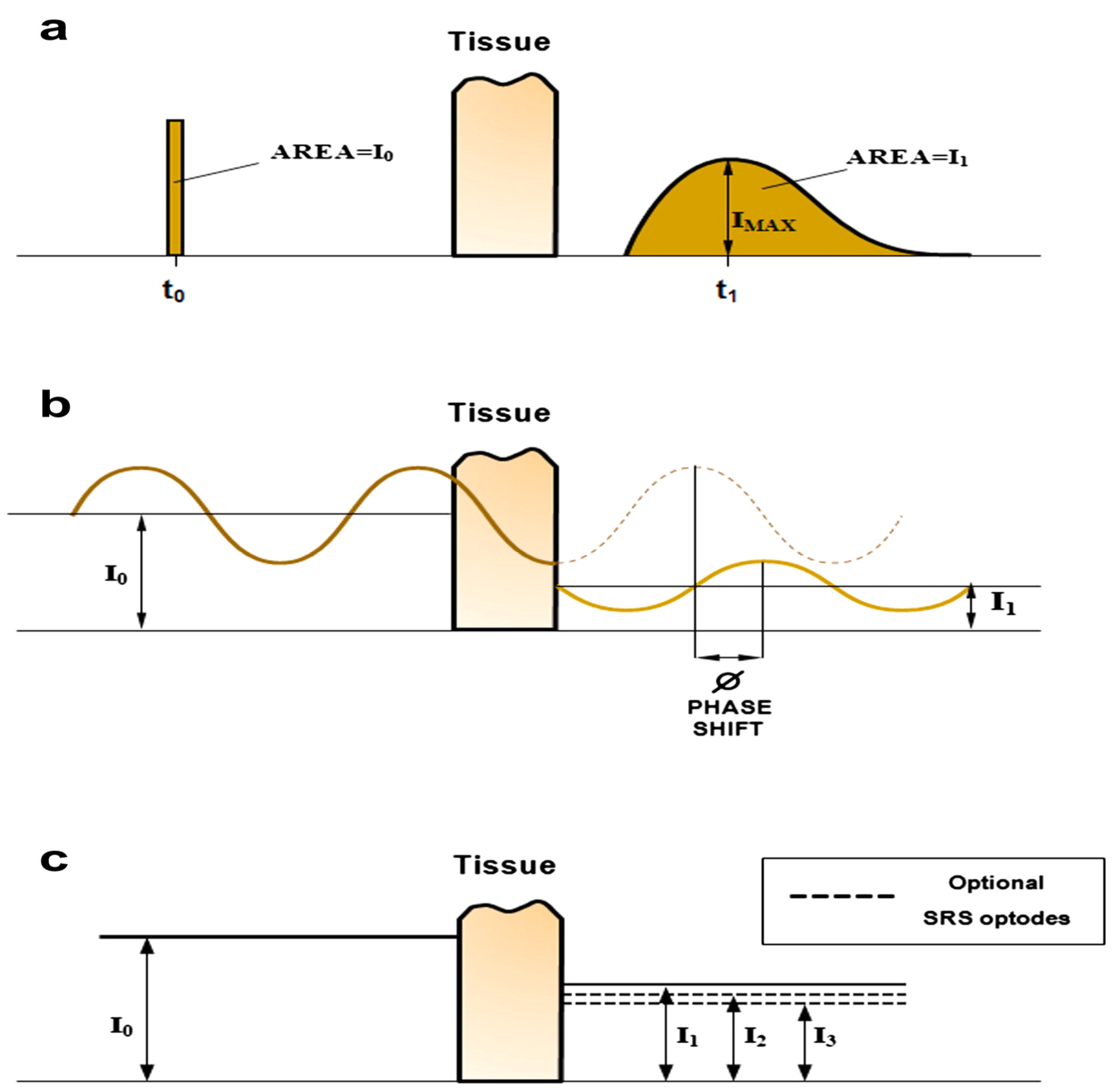
:1. Introduction
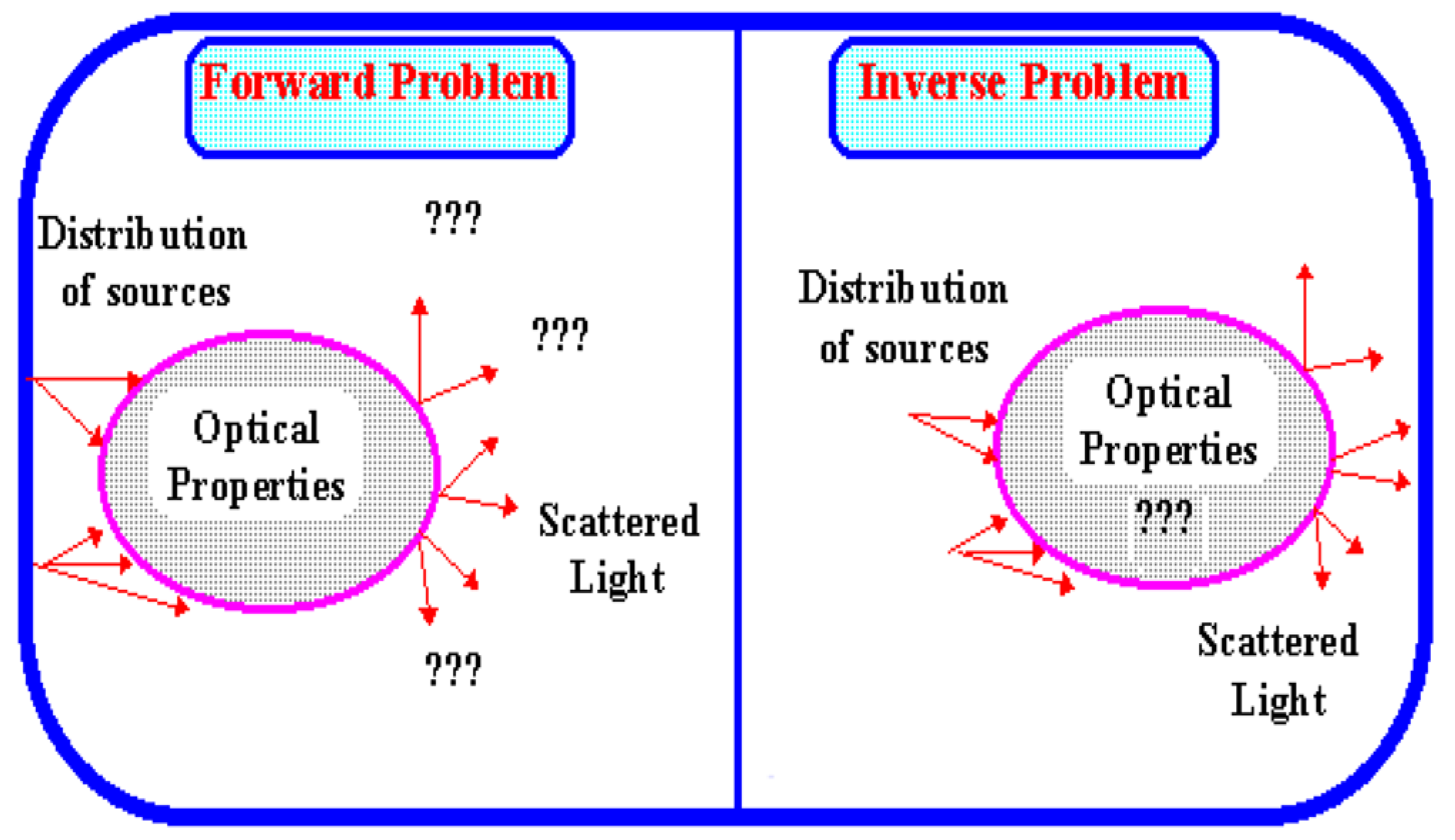
2. Mathematical Modeling of Light Transport in Biological Tissue as Forward Problem
3. Methods for Forward Model Simulation
3.1. Analytical Methods
3.2. Numerical Methods
3.2.1. Finite Difference Method
3.2.2. Finite Volume Method
3.2.3. Boundary Element Method
3.2.4. Finite Element Method
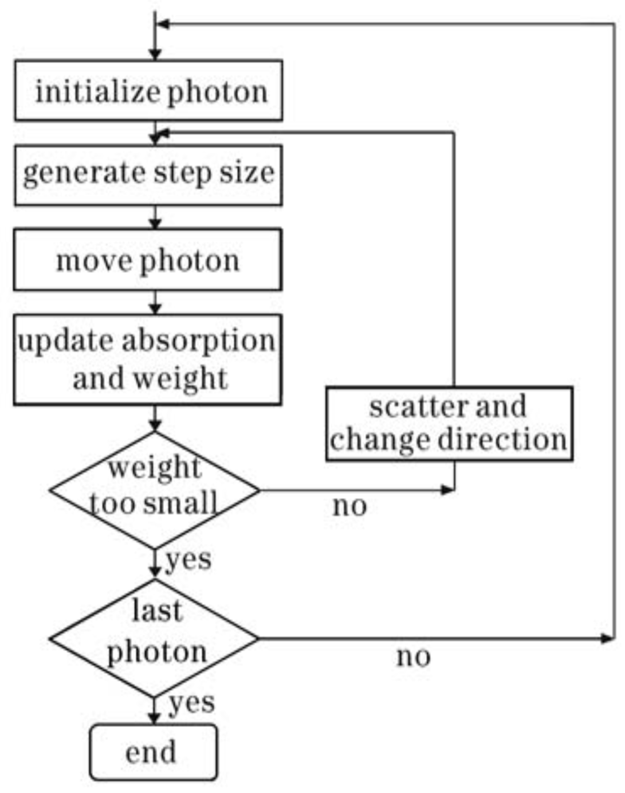
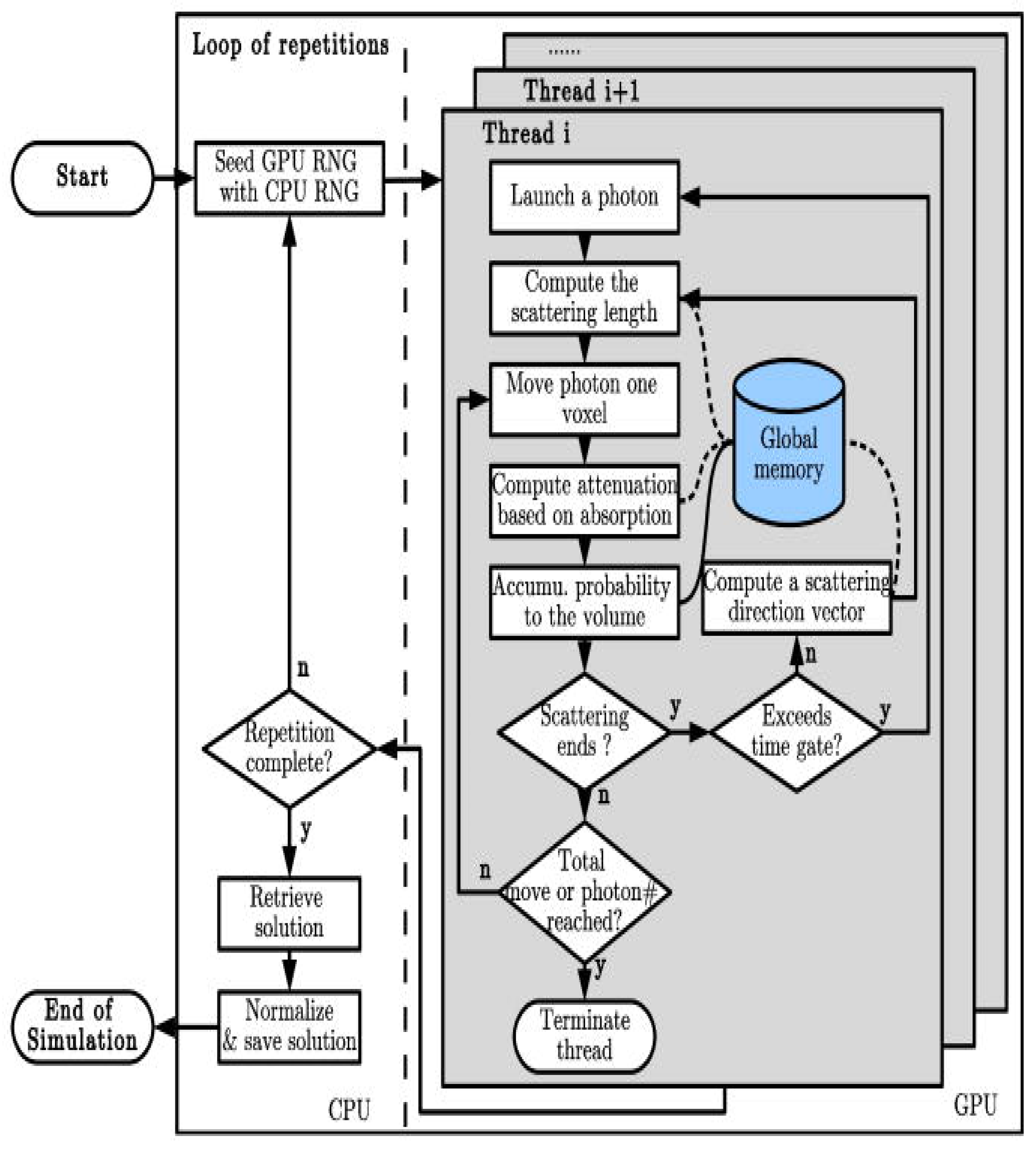
3.3. Stochastic Methods
4. Types of Toolboxes for Forward Model Simulation
4.1. MCML
4.2. NIRFAST
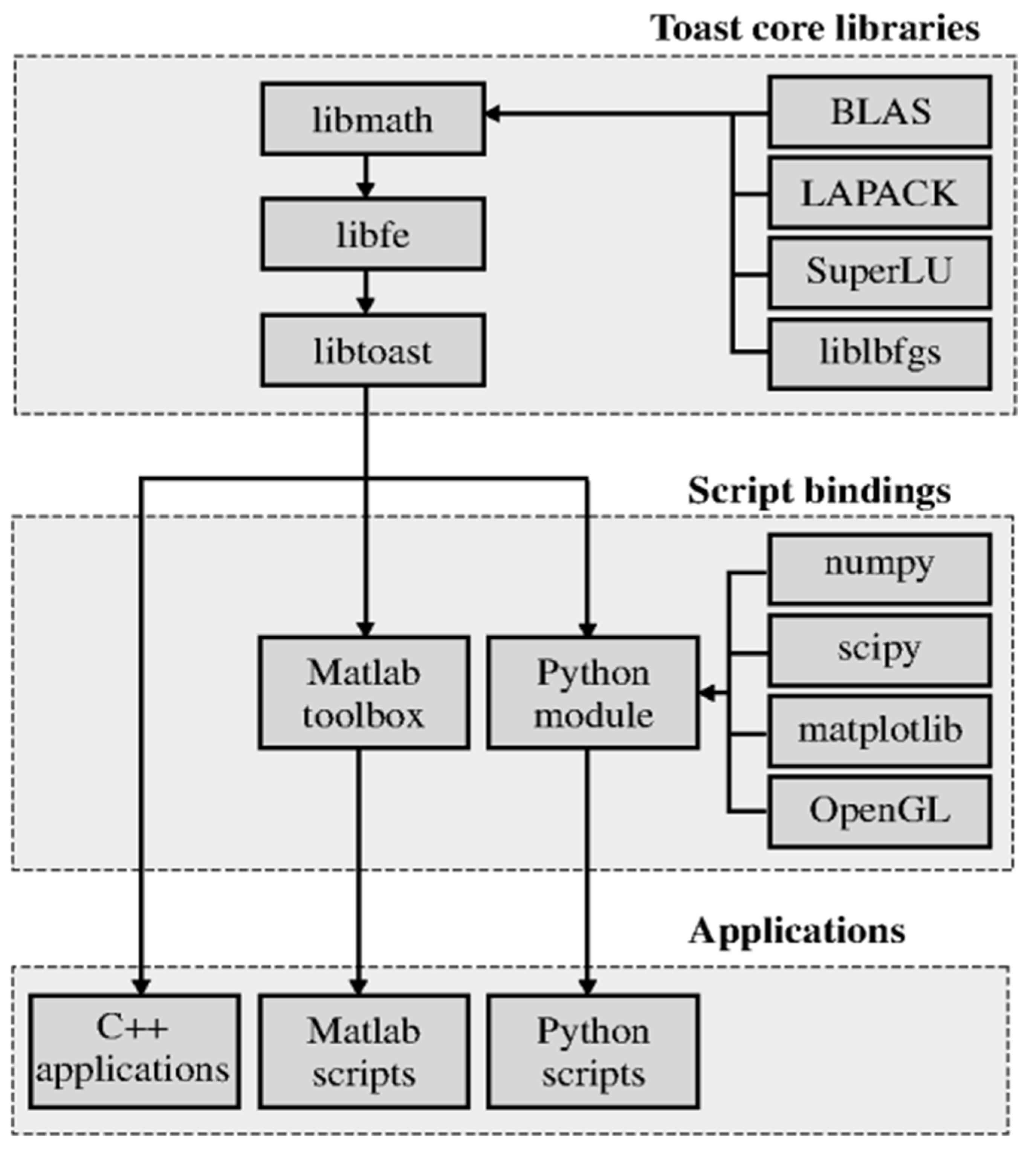
4.3. TOAST++
4.4. MCX/MMC
4.5. ValoMC
5. Inverse Problem
6. Methods for Inverse Problem Solution
6.1. Back Projection
6.2. Singular Value Decomposition (SVD) and Truncated Singular Value Decomposition (tSVD)
6.3. Least Square by QR Decomposition (LSQR) and Regularized LSQR (rLSQR)
6.4. Minimum Norm Estimate (MNE) and Weighted Minimum Norm Estimate (WMNE)
6.5. Low-Resolution Electromagnetic Tomographt (LORETA)
6.6. L1-Norm
6.7. Hierarchical Bayesian as MAP Estimate
- i.
- Considering the measurement noise as a Gaussian distribution and the forward problem as a probabilistic model aswhere is the covariance matrix.
- ii.
- Assuming the data prior distribution and likelihood function as and respectively.
- iii.
- Computation of the posterior distribution of the unknown aswhere anatomical prior image.
- iv.
- By applying the variational Bayesian (VB) method, the posterior could be written as variational free energywithimage by maximizing the free energy, providing the reconstruction, and applying the Bayes rule to the posterior distribution.
6.8. Expectation-Maximization (EM)
- ⮚
- E-step given the observed data and the current estimate , the conditional anticipation of the whole log-likelihood could be computed as
- ⮚
- M-step: Update the estimated value ofEquation can be explained separately for each element asis the element. It can be resolved using the soft threshold technique.
6.9. Maximum Entropy on the Mean (MEM)
6.10. Bayesian Model Averaging
- i.
- Consider the basic assumption of the Bayesian formulization of the given problem as a normal probability density function aswhere represents as hyperparameters which is unknown [11].
- ii.
- The estimation of the parameter as the first level of inference using the Bayes theorem is described as the posterior probability density function awhere represents as k-th model which is to be considered for the given problem.
- iii.
- The estimation of the hyperparameters as 2nd level of inference is describing as the posterior probability density function as
- iv.
- The estimation of the model as the third level of inference as the posterior probability density function
- v.
- Lastly, marginalizing the first, second, and third level of inference as posterior pdf as
7. Conclusions
Author Contributions
Funding
Data Availability Statement
Acknowledgments
Conflicts of Interest
References
- Ferrari, M.; Mottola, L.; Quaresima, V. Principles, techniques, and limitations of near infrared spectroscopy. Can. J. Appl. Physiol. 2004, 29, 463–487. [Google Scholar] [CrossRef] [PubMed]
- Wolf, M.; Ferrari, M.; Quaresima, V. Progress of near-infrared spectroscopy and topography for brain and muscle clinical applications. J. Biomed. Opt. 2007, 12, 062104. [Google Scholar] [PubMed]
- Bérubé-Lauzière, Y.; Crotti, M.; Boucher, S.; Ettehadi, S.; Pichette, J.; Rech, I. Prospects on time-domain diffuse optical tomography based on time-correlated single photon counting for small animal imaging. J. Spectrosc. 2016, 2016, 1947613. [Google Scholar] [CrossRef]
- Lo, P.A.; Chiang, H.K. Three-dimensional fluorescence diffuse optical tomography using the adaptive spatial prior approach. J. Med. Biol. Eng. 2019, 39, 827–834. [Google Scholar] [CrossRef]
- Applegate, M.; Istfan, R.; Spink, S.; Tank, A.; Roblyer, D. Recent advances in high speed diffuse optical imaging in biomedicine. APL Photonics 2020, 5, 040802. [Google Scholar] [CrossRef]
- Pellicer, A.; del Carmen Bravo, M. Near-infrared spectroscopy: A methodology-focused review. In Seminars in Fetal and Neonatal Medicine; Elsevier: Amsterdam, The Netherlands, 2011; Volume 16, pp. 42–49. [Google Scholar]
- Rahim, R.A.; Chen, L.L.; San, C.K.; Rahiman, M.H.F.; Fea, P.J. Multiple fan-beam optical tomography: Modelling techniques. Sensors 2009, 9, 8562–8578. [Google Scholar] [CrossRef]
- Klose, A.D.; Netz, U.; Beuthan, J.; Hielscher, A.H. Optical tomography using the time-independent equation of radiative transfer—Part 1: Forward model. J. Quant. Spectrosc. Radiat. Transf. 2002, 72, 691–713. [Google Scholar] [CrossRef]
- Hoshi, Y.; Yamada, Y. Overview of diffuse optical tomography and its clinical applications. J. Biomed. Opt. 2016, 21, 091312. [Google Scholar] [CrossRef]
- Arridge, S.R. Optical tomography in medical imaging. Inverse Probl. 1999, 15, R41. [Google Scholar] [CrossRef]
- Tremblay, J.; Martínez-Montes, E.; Vannasing, P.; Nguyen, D.K.; Sawan, M.; Lepore, F.; Gallagher, A. Comparison of source localization techniques in diffuse optical tomography for fNIRS application using a realistic head model. Biomed. Opt. Express 2018, 9, 2994–3016. [Google Scholar] [CrossRef]
- Madsen, S.J. Optical Methods and Instrumentation in Brain Imaging and Therapy; Springer Science & Business Media: Berlin/Heidelberg, Germany, 2012. [Google Scholar]
- Kavuri, V.C.; Lin, Z.-J.; Tian, F.; Liu, H. Sparsity enhanced spatial resolution and depth localization in diffuse optical tomography. Biomed. Opt. Express 2012, 3, 943–957. [Google Scholar] [CrossRef]
- Yamada, Y.; Suzuki, H.; Yamashita, Y. Time-domain near-infrared spectroscopy and imaging: A review. Appl. Sci. 2019, 9, 1127. [Google Scholar] [CrossRef]
- Patterson, M.S.; Chance, B.; Wilson, B.C. Time resolved reflectance and transmittance for the noninvasive measurement of tissue optical properties. Appl. Opt. 1989, 28, 2331–2336. [Google Scholar] [CrossRef] [PubMed]
- Arridge, S.R.; Hebden, J.C. Optical imaging in medicine: II. Modelling and reconstruction. Phys. Med. Biol. 1997, 42, 841. [Google Scholar] [CrossRef] [PubMed]
- Arridge, S.R.; Cope, M.; Delpy, D. The theoretical basis for the determination of optical pathlengths in tissue: Temporal and frequency analysis. Phys. Med. Biol. 1992, 37, 1531. [Google Scholar] [CrossRef] [PubMed]
- Sikora, J.; Zacharopoulos, A.; Douiri, A.; Schweiger, M.; Horesh, L.; Arridge, S.R.; Ripoll, J. Diffuse photon propagation in multilayered geometries. Phys. Med. Biol. 2006, 51, 497. [Google Scholar] [CrossRef]
- Liemert, A.; Kienle, A. Light diffusion in N-layered turbid media: Frequency and time domains. J. Biomed. Opt. 2010, 15, 025002. [Google Scholar] [CrossRef]
- Zhang, A.; Piao, D.; Bunting, C.F.; Pogue, B.W. Photon diffusion in a homogeneous medium bounded externally or internally by an infinitely long circular cylindrical applicator. I. Steady-state theory. JOSA A 2010, 27, 648–662. [Google Scholar] [CrossRef]
- Liemert, A.; Kienle, A. Light diffusion in a turbid cylinder. I. Homogeneous case. Opt. Express 2010, 18, 9456–9473. [Google Scholar] [CrossRef]
- Erkol, H.; Nouizi, F.; Unlu, M.; Gulsen, G. An extended analytical approach for diffuse optical imaging. Phys. Med. Biol. 2015, 60, 5103. [Google Scholar] [CrossRef]
- Arridge, S.R. Methods in diffuse optical imaging. Philos. Trans. R. Soc. A Math. Phys. Eng. Sci. 2011, 369, 4558–4576. [Google Scholar] [CrossRef] [PubMed]
- Martelli, F.; Sassaroli, A.; Yamada, Y.; Zaccanti, G. Analytical approximate solutions of the time-domain diffusion equation in layered slabs. JOSA A 2002, 19, 71–80. [Google Scholar] [CrossRef] [PubMed]
- Pogue, B.; Patterson, M.; Jiang, H.; Paulsen, K. Initial assessment of a simple system for frequency domain diffuse optical tomography. Phys. Med. Biol. 1995, 40, 1709. [Google Scholar] [CrossRef]
- Hielscher, A.H.; Alcouffe, R.E.; Barbour, R.L. Comparison of finite-difference transport and diffusion calculations for photon migration in homogeneous and heterogeneous tissues. Phys. Med. Biol. 1998, 43, 1285. [Google Scholar] [CrossRef] [PubMed]
- Hielscher, A.H.; Klose, A.D.; Hanson, K.M. Gradient-based iterative image reconstruction scheme for time-resolved optical tomography. IEEE Trans. Med. Imaging 1999, 18, 262–271. [Google Scholar] [CrossRef]
- Tanifuji, T.; Chiba, N.; Hijikata, M. FDTD (finite difference time domain) analysis of optical pulse responses in biological tissues for spectroscopic diffused optical tomography. In Proceedings of the Technical Digest. CLEO/Pacific Rim 2001. 4th Pacific Rim Conference on Lasers and Electro-Optics (Cat. No. 01TH8557), Chiba, Japan, 15–19 July 2001; p. TuD3_5. [Google Scholar]
- Tanifuji, T.; Hijikata, M. Finite difference time domain (FDTD) analysis of optical pulse responses in biological tissues for spectroscopic diffused optical tomography. IEEE Trans. Med. Imaging 2002, 21, 181–184. [Google Scholar] [CrossRef]
- Ichitsubo, K.; Tanifuji, T. Time-resolved noninvasive optical parameters determination in three-dimensional biological tissue using finite difference time domain analysis with nonuniform grids for diffusion equations. In Proceedings of the 2005 IEEE Engineering in Medicine and Biology 27th Annual Conference, Shanghai, China, 17–18 January 2006; pp. 3133–3136. [Google Scholar]
- Ren, K.; Abdoulaev, G.S.; Bal, G.; Hielscher, A.H. Algorithm for solving the equation of radiative transfer in the frequency domain. Opt. Lett. 2004, 29, 578–580. [Google Scholar] [CrossRef]
- Montejo, L.D.; Kim, H.-K.K.; Hielscher, A.H. A finite-volume algorithm for modeling light transport with the time-independent simplified spherical harmonics approximation to the equation of radiative transfer. In Proceedings of the Optical Tomography and Spectroscopy of Tissue IX, San Francisco, CA, USA, 22–27 January 2011; p. 78960J. [Google Scholar]
- Soloviev, V.Y.; D’Andrea, C.; Mohan, P.S.; Valentini, G.; Cubeddu, R.; Arridge, S.R. Fluorescence lifetime optical tomography with discontinuous Galerkin discretisation scheme. Biomed. Opt. Express 2010, 1, 998–1013. [Google Scholar] [CrossRef]
- Zacharopoulos, A.D.; Arridge, S.R.; Dorn, O.; Kolehmainen, V.; Sikora, J. Three-dimensional reconstruction of shape and piecewise constant region values for optical tomography using spherical harmonic parametrization and a boundary element method. Inverse Probl. 2006, 22, 1509. [Google Scholar] [CrossRef]
- Grzywacz, T.; Sikora, J.; Wojtowicz, S. Substructuring methods for 3-D BEM multilayered model for diffuse optical tomography problems. IEEE Trans. Magn. 2008, 44, 1374–1377. [Google Scholar] [CrossRef]
- Srinivasan, S.; Ghadyani, H.R.; Pogue, B.W.; Paulsen, K.D. A coupled finite element-boundary element method for modeling Diffusion equation in 3D multi-modality optical imaging. Biomed. Opt. Express 2010, 1, 398–413. [Google Scholar] [CrossRef]
- Srinivasan, S.; Carpenter, C.M.; Ghadyani, H.R.; Taka, S.J.; Kaufman, P.A.; Wells, W.A.; Pogue, B.W.; Paulsen, K.D. Image guided near-infrared spectroscopy of breast tissue in vivo using boundary element method. J. Biomed. Opt. 2010, 15, 061703. [Google Scholar] [CrossRef] [PubMed]
- Elisee, J.P.; Gibson, A.; Arridge, S. Combination of boundary element method and finite element method in diffuse optical tomography. IEEE Trans. Biomed. Eng. 2010, 57, 2737–2745. [Google Scholar] [CrossRef]
- Xie, W.; Deng, Y.; Lian, L.; Wang, K.; Luo, Z.; Gong, H. Boundary element method for diffuse optical tomography. In Proceedings of the 2013 Seventh International Conference on Image and Graphics, Qingdao, China, 26–28 July 2013; pp. 5–8. [Google Scholar]
- Arridge, S.; Schweiger, M.; Hiraoka, M.; Delpy, D. A finite element approach for modelig photon transport in tissue. Med. Phys. 1993, 20, 299–309. [Google Scholar] [CrossRef] [PubMed]
- Schweiger, M.; Arridge, S.R.; Delpy, D.T. Application of the finite-element method for the forward and inverse models in optical tomography. J. Math. Imaging Vis. 1993, 3, 263–283. [Google Scholar] [CrossRef]
- Jiang, H.; Paulsen, K.D. Finite-element-based higher order diffusion approximation of light propagation in tissues. In Proceedings of the Optical Tomography, Photon Migration, and Spectroscopy of Tissue and Model Media: Theory, Human Studies, and Instrumentation, San Jose, CA, USA, 1–28 February 1995; pp. 608–614. [Google Scholar]
- Schweiger, M.; Arridge, S.; Hiraoka, M.; Delpy, D. The finite element method for the propagation of light in scattering media: Boundary and source conditions. Med. Phys. 1995, 22, 1779–1792. [Google Scholar] [CrossRef] [PubMed]
- Gao, F.; Niu, H.; Zhao, H.; Zhang, H. The forward and inverse models in time-resolved optical tomography imaging and their finite-element method solutions. Image Vis. Comput. 1998, 16, 703–712. [Google Scholar] [CrossRef]
- Jiang, H. Frequency-domain fluorescent diffusion tomography: A finite-element-based algorithm and simulations. Appl. Opt. 1998, 37, 5337–5343. [Google Scholar] [CrossRef]
- Klose, A.D.; Hielscher, A.H. Iterative reconstruction scheme for optical tomography based on the equation of radiative transfer. Med. Phys. 1999, 26, 1698–1707. [Google Scholar] [CrossRef]
- Dehghani, H.; Srinivasan, S.; Pogue, B.W.; Gibson, A. Numerical modelling and image reconstruction in diffuse optical tomography. Philos. Trans. R. Soc. A Math. Phys. Eng. Sci. 2009, 367, 3073–3093. [Google Scholar] [CrossRef]
- Paulsen, K.D.; Jiang, H. Spatially varying optical property reconstruction using a finite element diffusion equation approximation. Med. Phys. 1995, 22, 691–701. [Google Scholar] [CrossRef]
- Gao, H.; Zhao, H. A fast-forward solver of radiative transfer equation. Transp. Theory Stat. Phys. 2009, 38, 149–192. [Google Scholar] [CrossRef]
- Wang, L.; Jacques, S.L.; Zheng, L. MCML—Monte Carlo modeling of light transport in multi-layered tissues. Comput. Methods Programs Biomed. 1995, 47, 131–146. [Google Scholar] [CrossRef] [PubMed]
- Chen, J.; Intes, X. Comparison of Monte Carlo methods for fluorescence molecular tomography—Computational efficiency. Med. Phys. 2011, 38, 5788–5798. [Google Scholar] [CrossRef]
- Chen, J.; Intes, X. Time-gated perturbation Monte Carlo for whole body functional imaging in small animals. Opt. Express 2009, 17, 19566–19579. [Google Scholar] [CrossRef]
- Periyasamy, V.; Pramanik, M. Advances in Monte Carlo simulation for light propagation in tissue. IEEE Rev. Biomed. Eng. 2017, 10, 122–135. [Google Scholar] [CrossRef]
- Dehghani, H.; Eames, M.E.; Yalavarthy, P.K.; Davis, S.C.; Srinivasan, S.; Carpenter, C.M.; Pogue, B.W.; Paulsen, K.D. Near infrared optical tomography using NIRFAST: Algorithm for numerical model and image reconstruction. Commun. Numer. Methods Eng. 2009, 25, 711–732. [Google Scholar] [CrossRef]
- Schweiger, M.; Arridge, S.R. The Toast++ software suite for forward and inverse modeling in optical tomography. J. Biomed. Opt. 2014, 19, 040801. [Google Scholar] [CrossRef]
- Fang, Q.; Boas, D.A. Monte Carlo simulation of photon migration in 3D turbid media accelerated by graphics processing units. Opt. Express 2009, 17, 20178–20190. [Google Scholar] [CrossRef] [PubMed]
- Fang, Q. Mesh-based Monte Carlo method using fast ray-tracing in Plücker coordinates. Biomed. Opt. Express 2010, 1, 165–175. [Google Scholar] [CrossRef] [PubMed]
- Yu, L.; Nina-Paravecino, F.; Kaeli, D.R.; Fang, Q. Scalable and massively parallel Monte Carlo photon transport simulations for heterogeneous computing platforms. J. Biomed. Opt. 2018, 23, 010504. [Google Scholar] [CrossRef] [PubMed]
- Yan, S.; Fang, Q. Hybrid mesh and voxel based Monte Carlo algorithm for accurate and efficient photon transport modeling in complex bio-tissues. Biomed. Opt. Express 2020, 11, 6262–6270. [Google Scholar] [CrossRef] [PubMed]
- Leino, A.A.; Pulkkinen, A.; Tarvainen, T. ValoMC: A Monte Carlo software and MATLAB toolbox for simulating light transport in biological tissue. OSA Contin. 2019, 2, 957–972. [Google Scholar] [CrossRef]
- Walker, S.A.; Fantini, S.; Gratton, E. Image reconstruction by backprojection from frequency-domain optical measurements in highly scattering media. Appl. Opt. 1997, 36, 170–179. [Google Scholar] [CrossRef] [PubMed]
- Boas, D.; Chen, K.; Grebert, D.; Franceschini, M. Improving the diffuse optical imaging spatial resolution of the cerebral hemodynamic response to brain activation in humans. Opt. Lett. 2004, 29, 1506–1508. [Google Scholar] [CrossRef] [PubMed]
- Zhai, Y.; Cummer, S.A. Fast tomographic reconstruction strategy for diffuse optical tomography. Opt. Express 2009, 17, 5285–5297. [Google Scholar] [CrossRef] [PubMed]
- Das, T.; Dileep, B.; Dutta, P.K. Generalized curved beam back-projection method for near-infrared imaging using banana function. Appl. Opt. 2018, 57, 1838–1848. [Google Scholar] [CrossRef]
- Habermehl, C.; Steinbrink, J.M.; Müller, K.-R.; Haufe, S. Optimizing the regularization for image reconstruction of cerebral diffuse optical tomography. J. Biomed. Opt. 2014, 19, 096006. [Google Scholar] [CrossRef]
- Gupta, S.; Yalavarthy, P.K.; Roy, D.; Piao, D.; Vasu, R.M. Singular value decomposition based computationally efficient algorithm for rapid dynamic near-infrared diffuse optical tomography. Med. Phys. 2009, 36, 5559–5567. [Google Scholar] [CrossRef]
- Zhan, Y.; Eggebrecht, A.T.; Culver, J.P.; Dehghani, H. Singular value decomposition based regularization prior to spectral mixing improves crosstalk in dynamic imaging using spectral diffuse optical tomography. Biomed. Opt. Express 2012, 3, 2036–2049. [Google Scholar] [CrossRef]
- Paige, C.C.; Saunders, M.A. LSQR: An algorithm for sparse linear equations and sparse least squares. ACM Trans. Math. Softw. TOMS 1982, 8, 43–71. [Google Scholar] [CrossRef]
- Hussain, A.; Faye, I.; Muthuvalu, M.S.; Boon, T.T. Least Square QR Decomposition Method for Solving the Inverse Problem in Functional Near Infra-Red Spectroscopy. In Proceedings of the 2021 IEEE 19th Student Conference on Research and Development (SCOReD), Kota Kinabalu, Malaysia, 23–25 November 2021; pp. 362–366. [Google Scholar]
- Prakash, J.; Yalavarthy, P.K. A LSQR-type method provides a computationally efficient automated optimal choice of regularization parameter in diffuse optical tomography. Med. Phys. 2013, 40, 033101. [Google Scholar] [CrossRef] [PubMed]
- Shaw, C.B.; Prakash, J.; Pramanik, M.; Yalavarthy, P.K. Least squares QR-based decomposition provides an efficient way of computing optimal regularization parameter in photoacoustic tomography. J. Biomed. Opt. 2013, 18, 080501. [Google Scholar] [CrossRef] [PubMed]
- Yalavarthy, P.K.; Pogue, B.W.; Dehghani, H.; Paulsen, K.D. Weight-matrix structured regularization provides optimal generalized least-squares estimate in diffuse optical tomography. Med. Phys. 2007, 34, 2085–2098. [Google Scholar] [CrossRef] [PubMed]
- Yalavarthy, P.K.; Pogue, B.W.; Dehghani, H.; Carpenter, C.M.; Jiang, S.; Paulsen, K.D. Structural information within regularization matrices improves near infrared diffuse optical tomography. Opt. Express 2007, 15, 8043–8058. [Google Scholar] [CrossRef] [PubMed]
- Yalavarthy, P.K.; Lynch, D.R.; Pogue, B.W.; Dehghani, H.; Paulsen, K.D. Implementation of a computationally efficient least-squares algorithm for highly under-determined three-dimensional diffuse optical tomography problems. Med. Phys. 2008, 35, 1682–1697. [Google Scholar] [CrossRef]
- Haufe, S.; Nikulin, V.V.; Ziehe, A.; Müller, K.-R.; Nolte, G. Combining sparsity and rotational invariance in EEG/MEG source reconstruction. NeuroImage 2008, 42, 726–738. [Google Scholar] [CrossRef]
- Pascual-Marqui, R.D.; Michel, C.M.; Lehmann, D. Low resolution electromagnetic tomography: A new method for localizing electrical activity in the brain. Int. J. Psychophysiol. 1994, 18, 49–65. [Google Scholar] [CrossRef]
- Prakash, J.; Shaw, C.B.; Manjappa, R.; Kanhirodan, R.; Yalavarthy, P.K. Sparse recovery methods hold promise for diffuse optical tomographic image reconstruction. IEEE J. Sel. Top. Quantum Electron. 2013, 20, 74–82. [Google Scholar] [CrossRef]
- Shaw, C.B.; Yalavarthy, P.K. Performance evaluation of typical approximation algorithms for nonconvex ℓ p-minimization in diffuse optical tomography. JOSA A 2014, 31, 852–862. [Google Scholar] [CrossRef]
- Okawa, S.; Hoshi, Y.; Yamada, Y. Improvement of image quality of time-domain diffuse optical tomography with lp sparsity regularization. Biomed. Opt. Express 2011, 2, 3334–3348. [Google Scholar] [CrossRef] [PubMed]
- Sato, M.-A.; Yoshioka, T.; Kajihara, S.; Toyama, K.; Goda, N.; Doya, K.; Kawato, M. Hierarchical Bayesian estimation for MEG inverse problem. NeuroImage 2004, 23, 806–826. [Google Scholar] [CrossRef]
- Guven, M.; Yazici, B.; Intes, X.; Chance, B. Hierarchical bayesian algorithm for diffuse optical tomography. In Proceedings of the 34th Applied Imagery and Pattern Recognition Workshop (AIPR’05), Washington, DC, USA, 19 October–21 December 2005; pp. 6–145. [Google Scholar]
- Calvetti, D.; Pragliola, M.; Somersalo, E.; Strang, A. Sparse reconstructions from few noisy data: Analysis of hierarchical Bayesian models with generalized gamma hyperpriors. Inverse Probl. 2020, 36, 025010. [Google Scholar] [CrossRef]
- Shimokawa, T.; Kosaka, T.; Yamashita, O.; Hiroe, N.; Amita, T.; Inoue, Y.; Sato, M.A. Hierarchical Bayesian estimation improves depth accuracy and spatial resolution of diffuse optical tomography. Opt. Express 2012, 20, 20427–20446. [Google Scholar] [CrossRef] [PubMed]
- Shimokawa, T.; Kosaka, T.; Yamashita, O.; Hiroe, N.; Amita, T.; Inoue, Y.; Sato, M.A. Extended hierarchical Bayesian diffuse optical tomography for removing scalp artifact. Biomed. Opt. Express 2013, 4, 2411–2432. [Google Scholar] [CrossRef] [PubMed]
- Aihara, T.; Shimokawa, T.; Ogawa, T.; Okada, Y.; Ishikawa, A.; Inoue, Y.; Yamashita, O. Resting-state functional connectivity estimated with hierarchical bayesian diffuse optical tomography. Front. Neurosci. 2020, 14, 32. [Google Scholar] [CrossRef]
- Yamashita, O.; Shimokawa, T.; Aisu, R.; Amita, T.; Inoue, Y.; Sato, M.-A. Multi-subject and multi-task experimental validation of the hierarchical Bayesian diffuse optical tomography algorithm. Neuroimage 2016, 135, 287–299. [Google Scholar] [CrossRef]
- Hiltunen, P.; Prince, S.; Arridge, S. A combined reconstruction–classification method for diffuse optical tomography. Phys. Med. Biol. 2009, 54, 6457. [Google Scholar] [CrossRef]
- Cao, N.; Nehorai, A.; Jacob, M. Image reconstruction for diffuse optical tomography using sparsity regularization and expectation-maximization algorithm. Opt. Express 2007, 15, 13695–13708. [Google Scholar] [CrossRef]
- Amblard, C.; Lapalme, E.; Lina, J.-M. Biomagnetic source detection by maximum entropy and graphical models. IEEE Trans. Biomed. Eng. 2004, 51, 427–442. [Google Scholar] [CrossRef]
- Grova, C.; Daunizeau, J.; Lina, J.-M.; Bénar, C.G.; Benali, H.; Gotman, J. Evaluation of EEG localization methods using realistic simulations of interictal spikes. Neuroimage 2006, 29, 734–753. [Google Scholar] [CrossRef] [PubMed]
- Chowdhury, R.A.; Lina, J.M.; Kobayashi, E.; Grova, C. MEG source localization of spatially extended generators of epileptic activity: Comparing entropic and hierarchical bayesian approaches. PLoS ONE 2013, 8, e55969. [Google Scholar] [CrossRef] [PubMed]
- Cai, Z.; Machado, A.; Chowdhury, R.A.; Spilkin, A.; Vincent, T.; Aydin, Ü.; Pellegrino, G.; Lina, J.-M.; Grova, C. Diffuse optical reconstructions of fNIRS data using Maximum Entropy on the Mean. bioRxiv 2021, 23, 2021-02. [Google Scholar] [CrossRef]
- Trujillo-Barreto, N.J.; Aubert-Vázquez, E.; Valdés-Sosa, P.A. Bayesian model averaging in EEG/MEG imaging. NeuroImage 2004, 21, 1300–1319. [Google Scholar] [CrossRef] [PubMed]
- Fragoso, T.M.; Bertoli, W.; Louzada, F. Bayesian model averaging: A systematic review and conceptual classification. Int. Stat. Rev. 2018, 86, 1–28. [Google Scholar] [CrossRef]


| References | Forward Simulation Method | Simulation Software/Toolbox | Data Type |
|---|---|---|---|
| B. W. Pogue et al., 1995 [61] | FDM | N/A | N/A |
| M. A. Ansari et al., 2014 [62] | BEM | N/A | N/A |
| Dehghani, Hamid, et al., 2009 [54] | FEM | NIRFAST | Breast model data |
| Yalavarthy, Phaneendra K. et al., 2007–2008 [7,63,64] | FEM | N/A | Phantom |
| Brigadoi, Sabrina, et al., [65] | FEM | Toast++ | Real resting-state data |
| Chiarelli, Antonio M., et al., 2016 [66] | FEM | NIRFAST | Phantom |
| Lu, Wenqi, Daniel Lighter, and Iain B. Styles. 2018 [67] | FEM | NIRFAST | Realistic simulation data |
| Machado, A., et al., 2018 [68] | MC | MCX | Realistic simulation data |
| Yu, Leiming, et al., 2018 [58] | MC | MCX | Phantom |
| Jiang, Jingjing, et al., 2020 [69] | MC and FEM | MCX and Toast++ | Silicon phantom experiment |
| Fu, Xiaoxue, and John E. Richards. 2021 [70] | MC | MCX | Realistic simulation data |
| Cai, Zhengchen, et al., 2021 [71] | MC | MCX | Realistic |
| Mazumder, Dibbyan, et al., 2021 [72] | MC | MCX | Realistic simulation data |
Disclaimer/Publisher’s Note: The statements, opinions and data contained in all publications are solely those of the individual author(s) and contributor(s) and not of MDPI and/or the editor(s). MDPI and/or the editor(s) disclaim responsibility for any injury to people or property resulting from any ideas, methods, instructions or products referred to in the content. |
© 2023 by the authors. Licensee MDPI, Basel, Switzerland. This article is an open access article distributed under the terms and conditions of the Creative Commons Attribution (CC BY) license (https://creativecommons.org/licenses/by/4.0/).
Share and Cite
Hussain, A.; Faye, I.; Muthuvalu, M.S.; Tang, T.B.; Zafar, M. Advancements in Numerical Methods for Forward and Inverse Problems in Functional near Infra-Red Spectroscopy: A Review. Axioms 2023, 12, 326. https://doi.org/10.3390/axioms12040326
Hussain A, Faye I, Muthuvalu MS, Tang TB, Zafar M. Advancements in Numerical Methods for Forward and Inverse Problems in Functional near Infra-Red Spectroscopy: A Review. Axioms. 2023; 12(4):326. https://doi.org/10.3390/axioms12040326
Chicago/Turabian StyleHussain, Abida, Ibrahima Faye, Mohana Sundaram Muthuvalu, Tong Boon Tang, and Mudasar Zafar. 2023. "Advancements in Numerical Methods for Forward and Inverse Problems in Functional near Infra-Red Spectroscopy: A Review" Axioms 12, no. 4: 326. https://doi.org/10.3390/axioms12040326