Article

A Coupled PDE-ODE Model for Nonlinear Transient Heat Transfer with Convection Heating at the Boundary: Numerical Solution by Implicit Time Discretization and Sequential Decoupling

1
Department of Computer Science, Faculty of Chemical and System Engineering, University of Chemical Technology and Metallurgy, 1756 Sofia, Bulgaria
2
Department of Chemical Engineering, Faculty of Chemical and System Engineering, University of Chemical Technology and Metallurgy, 1756 Sofia, Bulgaria
3
Department of Numerical Methods and Algorithms, Faculty of Mathematics and Informatics, Sofia University St. Kliment Ohridski, 1164 Sofia, Bulgaria
4
Department of Differential Equations, Institute of Mathematics, Budapest University of Technology and Economics, 1111 Budapest, Hungary
5
ELKH-ELTE NumNet Research Group, 1117 Budapest, Hungary
*
Author to whom correspondence should be addressed.
Axioms 2023, 12(4), 323; https://doi.org/10.3390/axioms12040323
Submission received: 20 February 2023 / Revised: 17 March 2023 / Accepted: 22 March 2023 / Published: 24 March 2023
(This article belongs to the Special Issue Computational Heat Transfer and Fluid Dynamics)

Abstract

:
This article considers heat transfer in a solid body with temperature-dependent thermal conductivity that is in contact with a tank filled with liquid. The liquid in the tank is heated by hot liquid entering the tank through a pipe. Liquid at a lower temperature leaves the tank through another pipe. We propose a one-dimensional mathematical model that consists of a nonlinear PDE for the temperature along the solid body, coupled to a linear ODE for the temperature in the tank, the boundary and the initial conditions. All equations are converted into a dimensionless form reducing the input parameters to three dimensionless numbers and a dimensionless function. A steady-state analysis is performed. To solve the transient problem, a nontrivial numerical approach is proposed whereby the differential equations are first discretized in time. This reduces the problem to a sequence of nonlinear two-point boundary value problems (TPBVP) and a sequence of linear algebraic equations coupled to it. We show that knowing the temperature in the system at time level n − 1 allows us to decouple the TPBVP and the corresponding algebraic equation at time level n. Thus, starting from the initial conditions, the equations are decoupled and solved sequentially. The TPBVPs are solved by FDM with the Newtonian method.
MSC:
65M06; 65M20; 65M22; 65L10; 35K20

1. Introduction

This work investigates transient heat transfer in a solid body [1] with temperature-dependent thermal conductivity. The body is in thermal contact with a tank filled with a liquid at temperature T . Through one pipe, liquid at a higher temperature is entering the tank. Through another pipe, liquid at temperature T is leaving the tank. Thus, the liquid in the tank is being heated. Systems like this are encountered in engineering and chemical engineering equipment, e.g., in hydronic heating devices and continuous stirred-tank reactors (CSTR) [2,3]. Due to the symmetry of the considered system, the temperature u in the solid body depends on one spatial variable only; hence, the problem is one-dimensional. Since the thermal conductivity of the sloid depends on u , the heat equation for the solid body is a nonlinear partial differential equation (PDE). Due to its importance, the equation has been studied extensively. Various numerical methods for solving the equation have been developed [4,5,6,7]. For particular cases, analytical techniques have been proposed [8,9,10]. At the liquid–solid contact surface, we apply a convection boundary condition [11]. This condition connects the temperature T in the bulk of the liquid with the temperature u and the temperature gradient u / x at the surface. In this work, we assume that the liquid in the tank is well stirred so that the temperature in the liquid remains essentially uniform in space throughout the process (perfect mixing, ideal CSTR [2,3]). Consequently, the energy-balance equation of the tank leads to a first-order linear ordinary differential equation (ODE) for the temperature in the liquid T ( t ) , where t is the time. The equation contains the unknown temperature u at the liquid–solid contact surface. Thus, we get a system with a coupled PDE and ODE. Coupled PDE-ODE systems are important in science and engineering and are often studied in connection with control problems of electromagnetic, mechanical, and chemical-reaction coupling [12,13,14,15,16,17]. Examples of systems modeled by coupled PDEs and ODEs can be found in [18,19,20]. In general, decoupling the PDE and the ODE is not a trivial task, and if possible, leads to a hard-to-handle integro-differential system [12]. In the literature, there are mainly two strategies for numerical solutions of nonlinear PDE-ODE systems. In the first strategy, called coupled, the PDE and the ODE are solved together. Broadly speaking, there are two ways to do this. We can discretize the whole system in the considered space-time domain, e.g., by using the finite difference method (FDM), and then solve the obtained nonlinear algebraic system using an iterative method, e.g., the Newtonian method. Alternatively, we can first linearize the whole system and then solve the obtained sequence of linear PDE-ODE subsystems, e.g., by FDM or the finite element method (FEM). Examples of techniques associated with the first strategy include the nonlinear multigrid method [7,21], the full approximation scheme (FAS) [22], the Newton multigrid method [23,24], and Newton-type linearization-based methods [25]. The second strategy, called decoupled, in the context of the considered problem, is the following. A guess is made for the temperature u on the contact surface as a function of time. Using this guess, we can solve the ODE, obtaining the temperature in the liquid T ( t ) . By substituting T ( t ) into the boundary condition (BC), we can solve the PDE, subject to the BC, separately from the ODE. The solution provides us with a new function for the temperature u at the surface. The procedure is repeated until convergence. In fact, the method is a fixed-point iteration method. Examples of problems solved by the second strategy can be found in [26,27,28]. This method is not recommended for strongly coupled systems.
In this work, we propose a new method to solve the coupled nonlinear PDE-ODE system that does not fall into either of the described strategies. First, analogously to the technique used in [29,30,31], the system is discretized in time using an implicit finite difference scheme. This results in a fully discretized ODE and a semi-discretized PDE. The equations discretized in this way, together with the boundary conditions, can be converted into a sequence of nonlinear two-point boundary value problems (TPBVP) [32,33,34,35,36,37,38,39] for the unknown temperature in the solid and a sequence of linear algebraic equations for the unknown temperature in the liquid. This, as shown in the article, effectively decouples the PDE and the ODE because knowing the temperature in the liquid and along the solid body at time level n 1 allows us to decouple and solve the TPBVP and the corresponding algebraic equation at time level n . Thus, by starting from the initial conditions and sequentially decoupling and solving the TPBVPs and the algebraic equations, we obtain the solution of the problem. Note that the method is essentially different from the method of lines (MOL) [11,40], which is a traditional numerical approach to solving parabolic (and other) PDEs, because the MOL first discretizes the PDE in space. This yields a system of first-order ODEs with initial conditions, i.e., an initial value problem (IVP). Then, to solve the IVP, one can use Runge–Kutta methods or other appropriate IVP techniques. Contrary to this approach, we first discretize the equations in time, thereby reducing the problem to a sequence of nonlinear TPBVPs. To solve the TPBVPs, we apply the FDM with the Newtonian method [34,35,36], but many other methods can be used. An advantage of the proposed approach is that at each time level, we only have to solve one nonlinear TPBVP. The Jacobian matrix for the Newtonian method is only N × N , where N is the number of the space mesh-points. The method is unconditionally stable, fast, and easy to implement.
This article is structured in the following way. Section 2 presents the physical system and the proposed mathematical model. In Section 3, all equations are converted into a dimensionless form, and the mathematical problem is formulated in terms of the dimensionless equations. A steady-state analysis is performed in Section 4. The proposed numerical method is presented in Section 5. In this section, we convert the PDE-ODE system into a sequence of TPBVPs. How to solve the TPBVPs through the FDM is shown in Section 6. In Section 7, several computer experiments are presented, and the results are discussed.

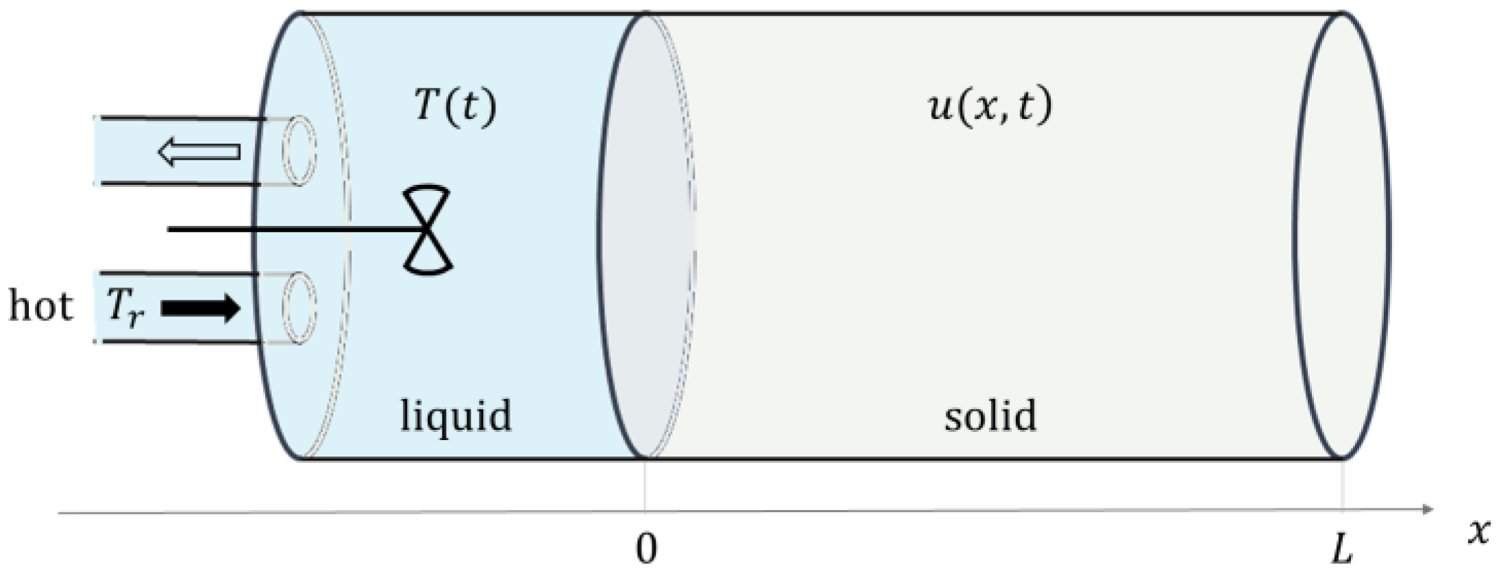
2. Physical System and Mathematical Model

The physical system considered in the article is the following. A cylindrical solid body is placed along the x -axis between x = 0 and x = L (Figure 1). The cylinder is laterally insulated. The temperature in the solid body is denoted by u x , t , where t is the time. Due to the symmetry of the problem, the temperature is a function of one spatial variable only. At x = 0 , the body is in thermal contact with a tank of volume V filled with liquid. The area of the contact surface is A . The temperature inside the tank is denoted by T t . The liquid in the tank is well stirred throughout the process, so the temperature is deemed essentially uniform in the bulk. Through one pipe, a hot liquid at temperature T r is entering the tank at a constant volumetric flow rate Q . Through another pipe, a liquid at temperature T t is leaving the tank at the same volumetric flow rate. Initially, the temperature in the body and in the tank is T 0 , where T 0 < T r . At x = L , the temperature is kept constant at T 0 , but other boundary conditions at x = L can also be applied.
The mathematical model describing the heat transfer in the system consists of the following equations. The heat equation for the solid body [1] is
ρ c p u x , t t = x κ u x , t u x , t x ,
where κ is the thermal conductivity of the solid body, ρ is its density, and c p is the specific heat capacity at constant pressure. The left-hand side of Equation (1) is the rate at which the energy density in the solid body at position x increases. It should be equal to the negative divergence of the heat flux vector at x , which in one dimension is just the right-hand side of Equation (1). Equation (1) is a PDE for the unknown temperature u x , t . In our model, κ depends on u ; hence, the PDE is nonlinear. The energy balance equation for the tank [2,3] is
d d t ρ l c p , l V T t Rate   of   energy   change = ρ l c p , l Q T r T t Rate   of   energy   input A H T t u 0 , t Rate   of   heat   loss   at   the   surface ,
where H is the mean convective heat transfer coefficient, which is considered constant. The density of the liquid is ρ l , and its specific heat capacity at constant pressure is c p , l . This is the well-known lumped capacitance model [1] applied to the liquid in the tank [2]. It follows naturally from the perfect mixing assumption [3], i.e., when no temperature gradient exists. The left-hand side of Equation (2) is the rate at which the energy in the tank increases. It equals the rate at which energy is entering the tank with the hot incoming liquid, minus the rate at which energy is leaving the tank with the outgoing liquid, minus the rate at which energy is being transferred from the liquid to the solid body through the contact surface. The transport of energy in the pipes is due to bulk motion of the fluid. This transport mechanism is called advection. The transport of energy from the liquid to the solid body is due to convection (convective heat transfer). Equation (2) is a linear ODE for the unknown temperature in the tank T t . This equation is coupled to the PDE in Equation (1) because it contains the temperature at the contact surface u 0 , t , which is an output variable (dependent variable) of Equation (1). At x = 0 , we apply the following convection boundary condition [1,11]:
κ u 0 , t u x , t x x = 0 = H T t u 0 , t .
Since κ depends on u , this condition is nonlinear. Note that, since Equation (3) contains the unknown temperature in the tank T t , we cannot solve the PDE, Equation (1), subject to the boundary condition, Equation (3), separately from the ODE, Equation (2). Hence, the PDE and the ODE are coupled. The initial conditions are
T 0 = T 0 , u x , 0 = T 0 .
At the right boundary, x = L , the temperature is kept constant at T 0 ; i.e.,
u L , t = T 0 .
The condition in Equation (5) is a Dirichlet boundary condition. Other boundary conditions, e.g., a fixed flux (Neumann-like) or a convection condition (Robin-like), can also be applied at x = L .
In the next section, in order to reduce the number of input parameters, we converted the equations into a dimensionless form. Then, the mathematical problem is formulated in terms of the dimensionless equations.

3. Dimensionless Equations and Formulation of the Mathematical Problem

The dimensionless temperature in the solid body and in the tank are defined as
Θ x , t = u x , t T 0 T r T 0 ,
Ψ t = T t T 0 T r T 0 ,
respectively. Note that u = T 0 and T = T 0 correspond to Θ = 0 and Ψ = 0 , respectively; and u = T r and T = T r to Θ = 1 and Ψ = 1 . Let
λ Θ x , t = κ u x , t .
Then, using Equations (6)–(8), Equations (1)–(3) become
Θ x , t t = x λ Θ x , t ρ c p Θ x , t x ,
d Ψ t d t = 1 t a 1 Ψ t 1 t c Ψ t Θ 0 , t ,
λ Θ 0 , t Θ x , t x x = 0 = H Ψ t Θ 0 , t ,
where
t a = V Q ,
t c = ρ l c p , l V H A .
both t a and t c have the dimension of time. The rate at which the temperature in the tank Ψ increases equals the difference of the two terms in Equation (10). The first one is due to energy transport by the liquid moving through the pipes (advection) and is inversely proportional to t a . Hence, t a is a characteristic time related to advection. The second term is due to convective heat transfer between the liquid and the solid body through the contact surface at x = 0 and is inversely proportional to t c . Hence, t c is a characteristic time related to convection. The right boundary condition is
Θ L , t = 0 .
the requirements that we impose on the thermal conductivity function λ Θ is that it is positive and twice continuously differentiable. Let the thermal conductivity at Θ = 0 be λ 0 . Then, the function λ Θ can be written in the form
λ Θ = λ 0 g Θ ,
where g C 2 0 , 1 is a dimensionless positive function with the property g 0 = 1 . To convert the thermal conductivity κ u into the form Equation (15), we have to solve Equation (6) for u and substitute it into Equation (8), thereby getting λ Θ . Then, g Θ = λ Θ / λ 0 , where λ 0 = λ 0 . Often, in engineering handbooks, the thermal conductivity is given in the form κ = κ 0 φ u / u r e f , where u r e f is some reference temperature. Then, λ 0 = κ 0 φ T 0 / u r e f . More information on temperature-dependent thermal conductivity can be found in [10].
The dimensionless position and the dimensionless time are defined as
ξ = x L ,         τ = t t ¯ ,
where
t ¯ = ρ c p L 2 λ 0 .
the dimensionless time variable τ is the Fourier number [41] at reference temperature T 0 ( θ = 0 ). Using the new variables ξ and τ , and
θ ξ , τ = Θ x , t , ψ τ = Ψ t ,
Equations (9)–(11), the boundary condition, Equation (14), and the initial conditions yield
θ ξ , τ τ = ξ g θ ξ , τ θ ξ , τ ξ ,
d ψ τ d τ = 1 τ a 1 ψ τ 1 τ c ψ τ θ 0 , τ ,
g θ 0 , τ θ ξ , τ ξ ξ = 0 = B i ψ τ θ 0 , τ ,
θ 1 , τ = 0 ,
ψ 0 = 0 ,       θ ξ , 0 = 0 ,
where
B i = H L λ 0
is the Biot number [42] at reference temperature T 0 ( θ = 0 ), and
τ a = t a t ¯ ,       τ c = t c t ¯
are dimensionless characteristic times. In Equations (19)–(21), the parameters τ a , τ c , and B i are given positive numbers, and g C 2 0 , 1 is a given positive function. We have to find θ ξ , τ and ψ τ by solving the system of Equations (19)–(23). The system consists of a nonlinear PDE, Equation (19); a coupled linear ODE, Equation (20); a nonlinear boundary condition, Equation (21), which couples the PDE to the ODE; a homogenous boundary condition, Equation (22); and initial conditions, Equation (23).
Formally, the solution of the ODE Equation (20), subject to the first initial condition in Equation (23), can be written as
ψ τ = 0 τ 1 τ a + θ 0 , s τ c e 1 τ a + 1 τ c s τ d s .
that Equation (26) is a solution to Equation (20) can easily be checked by direct substation. The problem with Equation (26) is that the function θ 0 , s is unknown; hence, the integration cannot be performed. Substituting Equation (26) into the boundary condition Equation (21) decouples the PDE, Equation (19), subject to boundary conditions, Equations (21) and (22), from the ODE, Equation (20), but this leads to an integro-differential system which is hard to handle. In Section 5, we propose a numerical approach for solving the system of Equations (19)–(23).

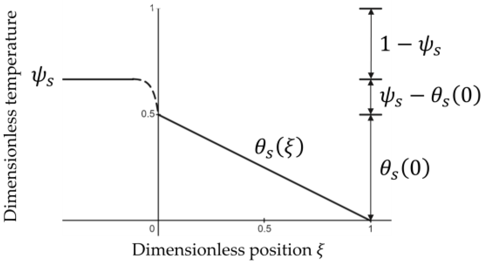
4. Steady-State Analysis

Let the steady-state temperature in the tank be ψ s , and in the solid body θ s ξ :
ψ s = lim τ ψ τ ,         θ s ξ = lim τ θ ξ , τ .
since ψ s is independent of time, Equation (20) becomes
1 τ a 1 ψ s 1 τ c ψ s θ s 0 = 0 .
taking into account that τ a / τ c = t a / t c , the equation can be written as
t a t c = 1 ψ s ψ s θ s 0 .
since the function θ s ξ is independent of time, the heat equation for the solid body Equation (19) becomes
d d ξ g θ s d θ s d ξ = 0 .
let us consider the case g θ 1 . Then, taking into account the second boundary condition, θ s 1 = 0 , the solution is
θ s ξ = θ s 0 1 ξ .
the temperature gradient is
d θ s ξ d ξ = θ s 0 .
therefore, the convection boundary condition, Equation (21), becomes
B i = θ s 0 ψ s θ s 0 .
Equation (33), which holds for g θ 1 , and Equation (29), uniquely determine the steady-state temperature in the tank ψ s and on the liquid–solid surface θ s 0 . As an example, in Figure 2, we show the steady-state temperature profile for the case where B i = 3 and t a / t c = 2 ; hence, by Formulas (29) and (33), ψ s = 2 / 3 and θ s 0 = 1 / 2 . On the right, the temperature intervals 0 , θ s 0 , θ s 0 , ψ s , and ψ s , 1 are depicted. The ratio of the length of the lower interval to the length of the middle interval equals the Biot number, B i , Equation (33)—i.e., three. The ratio of the length of the upper interval to the length of the middle interval equals the ratio t a / t c in Equation (29), i.e., two.

5. Implicit Time Discretization and Sequential Decoupling

We introduce a time-mesh τ n = n τ , n = 0 , 1 , 2 , , where τ is the time-step, and discretize the PDE, Equation (19), and the ODE, Equation (20), by replacing the time derivatives with the backward finite differences. At τ = τ n , n 1 , we have
θ ξ , τ n θ ξ , τ n 1 τ + O τ = d d ξ g θ ξ , τ n d θ ξ , τ n d ξ ,
ψ τ n ψ τ n 1 τ + O τ = 1 τ a 1 ψ τ n 1 τ c ψ τ n θ 0 , τ n ,
where τ a and τ c are defined in Equation (25). The proposed discretization scheme is implicit. This ensures unconditional stability of the numerical method. Let ψ n 1 and the function θ n 1 ξ be some suitable approximations for ψ τ n 1 and θ ξ , τ n 1 . By dropping the O τ terms in Equations (34) and (35) and supplementing the two equations with the boundary conditions Equations (21) and (22) at τ = τ n , we obtain
θ n ξ θ n 1 ξ τ = θ g θ n ξ d θ n ξ d ξ 2 + g θ n ξ d 2 θ n ξ d ξ 2 ,
g θ n 0 d θ n ξ d ξ ξ = 0 = B i ψ n θ n 0 ,
θ n 1 = 0 ,
ψ n ψ n 1 τ = 1 τ a 1 ψ n 1 τ c ψ n θ n 0 ,
where ψ n and θ n ξ are approximations for ψ τ n and θ ξ , τ n , respectively. Equation (36) is a nonlinear second-order ODE for the unknown function θ n ξ . The ODE in Equation (36), together with the boundary conditions of Equations (37) and (38), constitute a nonlinear TPBVP. Equation (39) is a linear algebraic equation for the unknown ψ n . Note that the TPBVP in Equations (36)–(38) contains the unknown ψ n , and Equation (39) contains the unknown θ n 0 ; hence, Equations (36)–(38) and Equation (39) are coupled. Unlike the original system in Equations (19)–(22), however, the system in Equations (36)–(39) allows easy decoupling, provided ψ n 1 is known. First, we express Equation (39) in the form
ψ n = R ψ n 1 τ + 1 τ a + θ n 0 τ c ,
where
R = 1 τ + 1 τ a + 1 τ c 1 .
substituting ψ n Equation (40) into the first boundary condition of Equation (37), the TPBVP in Equations (36)–(38) is transformed into
d 2 θ n ξ d ξ 2 = f θ n ξ , d θ n ξ d ξ ; θ n 1 ξ ,
g θ n 0 d θ n ξ d ξ ξ = 0 = B i R ψ n 1 τ + 1 τ a + θ n 0 τ c θ n 0 ,
θ n 1 = 0 ,
where, for convenience, we have rewritten Equation (36) in the form of Equation (42) by introducing the function
f θ n ξ , d θ n ξ d ξ ; θ n 1 ξ = 1 g θ n ξ θ n ξ θ n 1 ξ τ θ g θ n ξ d θ n ξ d ξ 2 .
since ψ n 1 in Equation (43) is just a known number, the TPBVP in Equations (42)–(44), unlike Equations (36)–(38), contains only the unknown θ n ξ ; hence, it is no longer coupled to the algebraic equation in Equation (39). If θ n 1 ξ is given, we can solve the TPBVP in Equations (42)–(44), obtaining θ n ξ . Then, using θ n 0 in Equation (40), we can obtain ψ n . In other words, by knowing the temperature in the tank and along the solid body at time level n 1 , we can decouple and solve the TPBVP Equations (42)–(44), obtaining the temperature along the solid body at time level n . Then, using the temperature on the liquid–solid contact surface at time level n , we can find, using Equation (40), the temperature in the tank at time level n . For n = 1 , 2 , . Equations (42)–(44) represent a sequence of TPBVPs, and Equation (40) is a sequence of algebraic equations. Starting from the initial conditions ψ 0 = 0 , θ 0 ξ = 0 , we can solve the TPBVP of Equations (42)–(44) at time level n = 1 and obtain θ 1 ξ , and then, using Equation (40), ψ 1 . Next, using ψ 1 and θ 1 ξ , we can solve the TPBVP for n = 2 , obtaining θ 2 ξ and then ψ 2 , and so on. Thus, sequentially, we decouple and solve the TPBVPs and the algebraic equations. This is the essence of the proposed numerical method. In fact, using the described procedure, the solution of the nonlinear coupled PDE-ODE system of Equations (19)–(23) comes down to solving, at each time level n, the nonlinear TPBVP of Equations (42)–(44).
In the literature, there are many methods for numerical solutions of nonlinear TPBVPs [32,33,34,35,36,37,38,39]. Some of them linearize the ODE, e.g., by quasi-linearization [37] or Picard linearization [35], and then solve the sequence of linear sub-problems by some linear method, e.g., the collocation method [33] or the linear shooting-method [34]. Other methods rely on replacing the TPBVP with a sequence of initial value problems, e.g., the shooting by Newtonian method (nonlinear shooting method) [38] and the shooting-projection method [39]. The finite difference method (FDM) [34,35,36] is another important method whereby the ODE is first discretized using finite differences, and then the obtained nonlinear system is solved iteratively, e.g., by the Newtonian method. In this paper, we adopt the FDM because it is reliable, it is easy to implement, and it can handle a large variety of boundary conditions, including the nonlinear condition of Equation (43). Not all available nonlinear methods are appropriate for problems such as Equations (42)–(44), so as explained in [29], caution should be exercised when choosing the particular numerical technique.

6. Solving the TPBVP via the FDM

We are going to solve the TPBVP in Equations (42)–(44) by the FDM with the Newton iteration method for the solution of the arising nonlinear algebraic systems. For the Newtonian method, we will need the partial derivatives of the function f in Equation (45), so we calculate them here. The partial derivative of f with respect to the first variable θ n is
1 f θ n ξ , d θ n ξ d ξ ; θ n 1 ξ = 1 g θ n ξ 2 1 τ θ θ 2 g θ n ξ d θ n ξ d ξ 2 g θ n ξ θ n ξ θ n 1 ξ τ θ g θ n ξ d θ n ξ d ξ 2 θ g θ n ξ = 1 g θ n ξ 1 τ θ θ 2 g θ n ξ d θ n ξ d ξ 2 f θ n ξ , d θ n ξ d ξ ; θ n 1 ξ θ g θ n ξ .
the partial derivative of f with respect to the second variable d θ n / d ξ is
2 f θ n ξ , d θ n ξ d ξ = 2 θ g θ n ξ g θ n ξ d θ n ξ d ξ .

6.1. Discretizing the TPBVP with the FDM

We introduce the space mesh:
ξ i = i 1 ξ , i = 1 , 2 , , N , ξ = 1 N 1 .
using the central difference approximations for d θ n ξ / d ξ and d 2 θ n ξ / d ξ 2 , the ODE of Equation (42) is discretized on the mesh in Equation (48):
θ n , i + 1 2 θ n , i + θ n , i 1 ξ 2 = f θ n , i , D θ n , i ; θ n 1 , i , i = 2 , 3 , , N 1 .
where
D θ n , i = θ n , i + 1 θ n , i 1 2 ξ .
in Equation (49) the unknowns θ n , i approximate θ n ξ i with approximation error O ξ 2 . The boundary condition, Equation (43), using O ξ 2 forward difference approximation for the first derivative d θ n ξ / d ξ , yields
g θ n , 1 D θ n , 1 = B i R ψ n 1 τ + 1 τ a + θ n , 1 τ c θ n , 1 ,
where
D θ n , 1 = θ n , 3 + 4 θ n , 2 3 θ n , 1 2 ξ .
the second boundary condition is
θ n , N = 0 .
altogether, Equations (49), (51), and (53) make a system of N algebraic equations for the N unknowns θ n , i , i = 1 , 2 , , N . The system is nonlinear.

6.2. Solving the Nonlinear System via the Newton Method

We introduce the vector F n = [ F n , 1 , F n , 2 , , F n , N ] T with components
F n , i = θ n , i + 1 2 θ n , i + θ n , i 1 ξ 2 f θ n , i , D θ n , i ; θ n 1 , i , i = 2 , 3 , , N 1 ,
F n , 1 = ξ g θ n , 1 D θ n , 1 + B i R ψ n 1 τ + 1 τ a + θ n , 1 τ c θ n , 1 , F n , N = θ n , N .
using Equations (54) and (55), the nonlinear system in Equations (49), (51), and (53) can be written as
F n θ n = 0 ,
where θ n = θ n , 1 , θ n , 2 , , θ n , N T . Let θ n ( k ) be an approximation of θ n . By expanding F n θ n in Equation (56) around θ n ( k ) , we get
F n θ n ( k ) + J n ( k ) θ n θ n ( k ) + = 0
where J n ( k ) is the Jacobian of F n with respect to θ n evaluated at θ n ( k ) :
J n ( k ) = F n θ n θ n k .
by replacing in Equation (57) θ n by θ n ( k + 1 ) and dropping the higher order terms, we obtain
θ n ( k + 1 ) = θ n ( k ) + δ θ n ( k ) , k = 0 , 1 , 2 ,
where
δ θ n ( k ) = J n k 1 F n θ n k .
this is the Newtonian iteration formula. In Equation (59), θ n ( k + 1 ) is the next, in general better, approximation of θ n . As an initial approximation θ n ( 0 ) , we use θ n 1 , i.e., the solution obtained at the previous time level.
Starting from θ n ( 0 ) , we can find each next approximation θ n ( k + 1 ) , k = 0 , 1 , , using Equation (59). If the sequence is convergent, then the limiting vector θ n = l i m θ n ( k ) , k is a solution to the system in Equations (49), (51), and (53). In practice, the iteration process is terminated when δ θ n ( k ) < ϵ , where · is some suitably chosen norm, e.g., the maximum norm, and ϵ is some small number. This inequality is called a stopping criterion. The vector θ n ( k + 1 ) is taken as an approximate solution to the system.

6.3. Calculating the Elements of the Jacobian

Using Equation (54), we get the nonzero elements of rows i = 2 , 3 , N 1 of the Jacobian equation—Equation (58):
J n i , i 1 k = F n , i θ n , i 1 θ n = θ n k = θ n , i 1 θ n , i + 1 2 θ n , i + θ n , i 1 ξ 2 f θ n , i , D θ n , i ; θ n 1 , i θ n = θ n k = 1 ξ 2 1 f θ n , i , D θ n , i ; θ n 1 , i θ n , i θ n , i 1 + 2 f θ n , i , D θ n , i D θ n , i θ n , i 1 θ n = θ n k = = 1 + ξ 2 2 f θ n , i k , D θ n , i k = 1 + ξ 2 p n , i k ,
J n i , i k = F n , i θ n , i θ n = θ n k = θ n , i θ n , i + 1 2 θ n , i + θ n , i 1 ξ 2 f θ n , i , D θ n , i ; θ n 1 , i θ n = θ n k = 2 ξ 2 1 f θ n , i , D θ n , i ; θ n 1 , i θ n , i θ n , i + 2 f θ n , i , D θ n , i D θ n , i θ n , i θ n = θ n k = 2 ξ 2 1 f θ n , i k , D θ n , i k = 2 ξ 2 q n , i k ,
J n i , i + 1 k = F n , i θ n , i + 1 θ n = θ n k = θ n , i + 1 θ n , i + 1 2 θ n , i + θ n , i 1 ξ 2 f θ n , i , D θ n , i ; θ n 1 , i θ n = θ n k = 1 ξ 2 1 f θ n , i , D θ n , i ; θ n 1 , i θ n , i θ n , i + 1 + 2 f θ n , i , D θ n , i D θ n , i θ n , i + 1 θ n = θ n k = 1 ξ 2 2 f θ n , i k , D θ n , i k = 1 ξ 2 p n , i k .
in the above formulas,
D θ n , i k = θ n , i + 1 k θ n , i 1 k 2 ξ , i = 2 , 3 , , N 1 ,
q n , i k = 1 f θ n , i k , D θ n , i k ; θ n 1 , i = 1 g θ n , i k 1 τ θ θ 2 g θ n , i k D θ n , i k 2 f θ n , i k , D θ n , i k ; θ n 1 , i θ g θ n , i k ,
p n , i k = 2 f θ n , i k , D θ n , i k = 2 θ g θ n , i k g θ n , i k D θ n , i k ,
where
f θ n , i k , D θ n , i k ; θ n 1 , i = 1 g θ n , i k θ n , i k θ n 1 , i τ θ g θ n , i k D θ n , i k 2 .
the first row of the Jacobian equation, Equation (58), concerns the first boundary condition. Using the first equation in Equation (55), we obtain the nonzero elements of the first row:
J n 1 , 1 k = F n , 1 θ n , 1 θ n = θ n k = ξ θ g θ n , 1 D θ n , 1 + g θ n , 1 D θ n , 1 θ n , 1 + B i R τ c 1 θ n = θ n k = 1 2 θ g θ n , 1 k θ n , 3 k + 4 θ n , 2 k 3 θ n , 1 k 3 2 g θ n , 1 k + B i R τ c 1 ξ ,
J n ( 1 , 2 ) ( k ) = F n , 1 θ n , 2 θ n = θ n k = ξ g θ n , 1 D θ n , 1 θ n , 2 θ n = θ n k = 2 g θ n , 1 k ,
J n ( 1 , 3 ) ( k ) = F n , 1 θ n , 3 θ n = θ n k = ξ g θ n , 1 D θ n , 1 θ n , 3 θ n = θ n k = 1 2 g θ n , 1 k .
the last row of the Jacobian concerns the second boundary condition. Using the second equation in Equation (55), we obtain the only nonzero element of the last row:
J n ( N , N ) ( k ) = F n , N θ n , N θ n = θ n k = 1 .

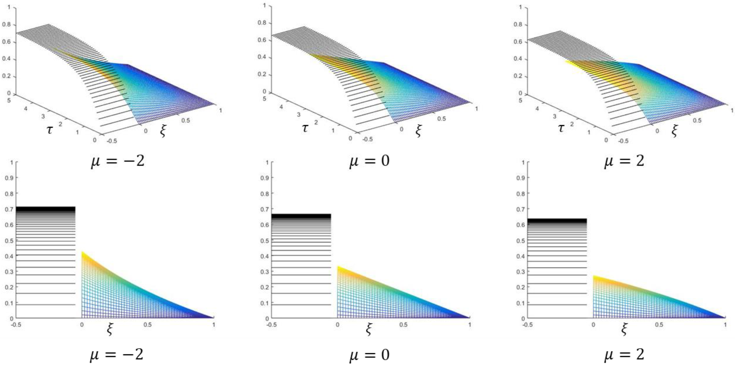
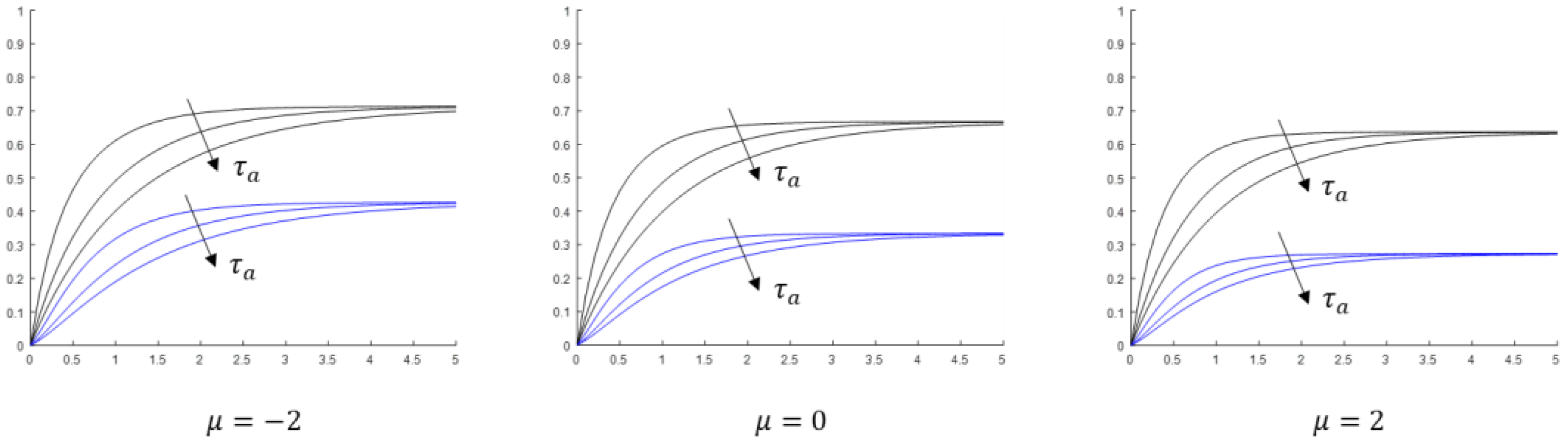
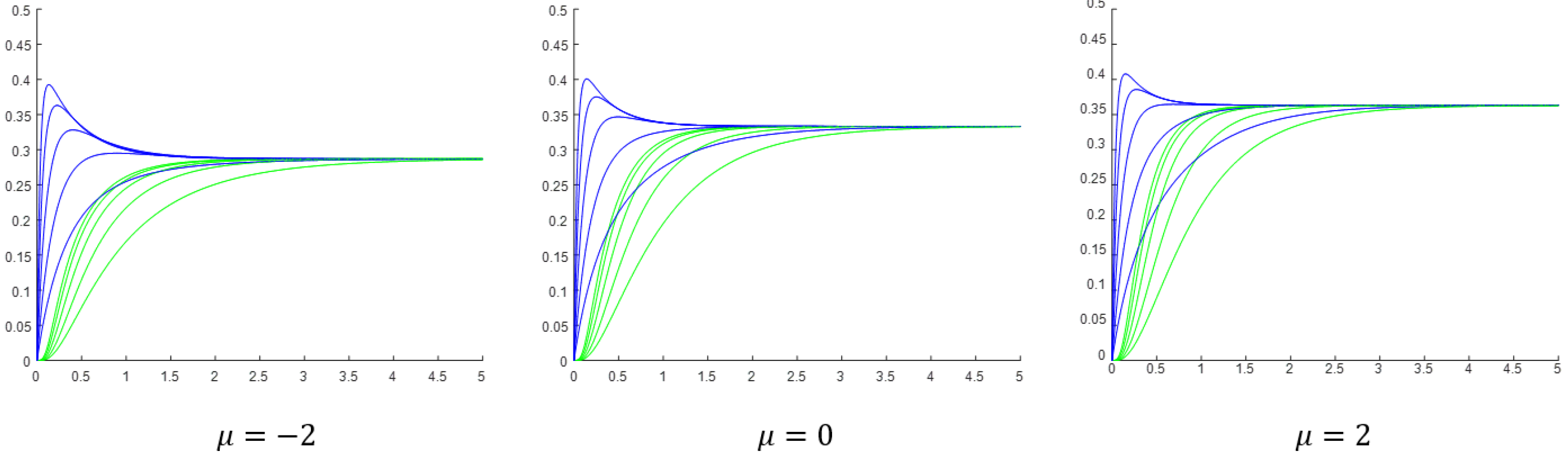
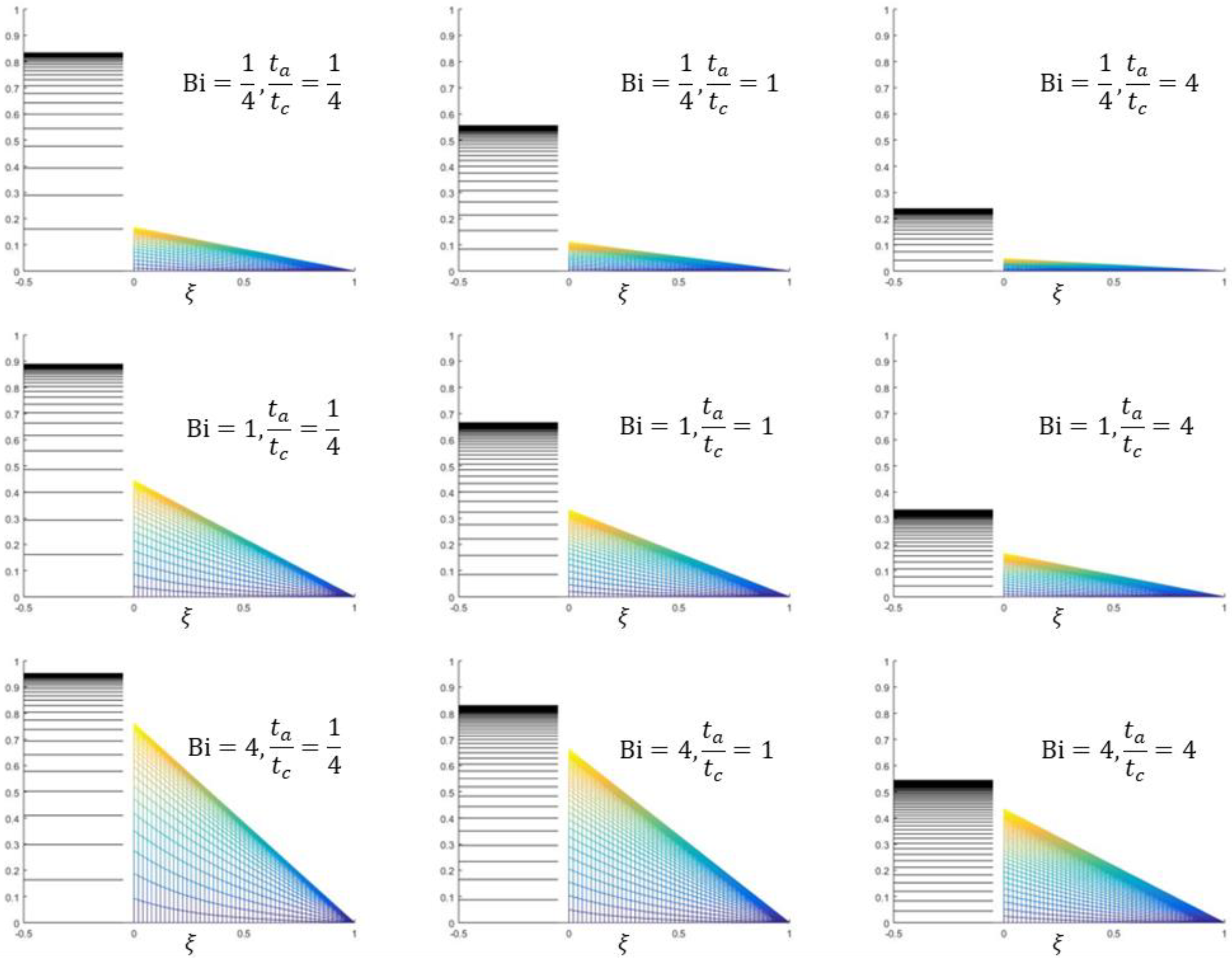
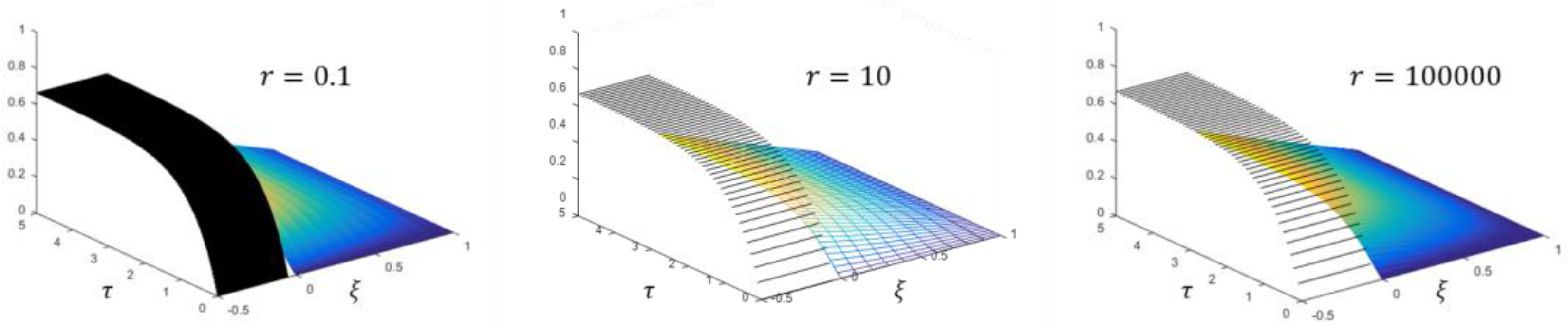
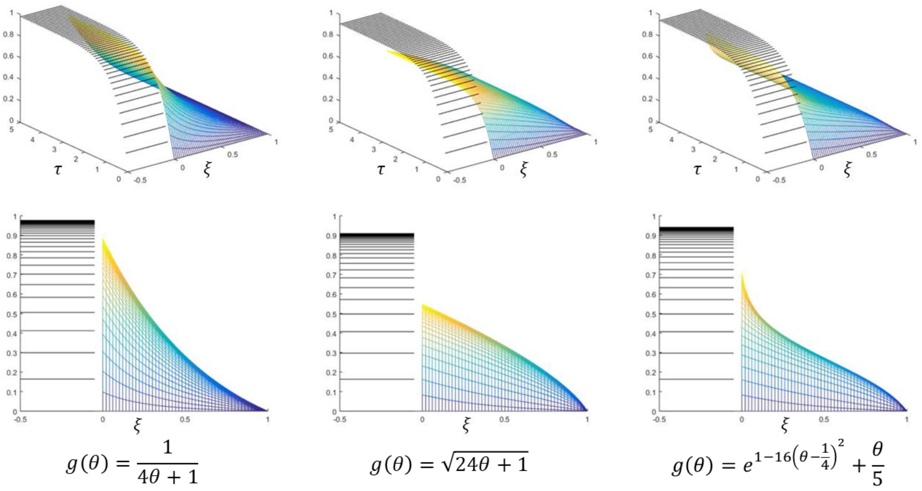
7. Computer Experiments and Discussion

In this section, we apply the proposed numerical approach to solve several examples and discuss the obtained results. A MATLAB implementation of the numerical method is given in Appendix A.
  • Example 1
In this example, we consider dimensionless thermal conductivity of the form
g θ = e μ θ .
problems with exponential dependence of the thermal conductivity on the temperature can be found in [43,44]. Such dependence occurs in some materials, e.g., in silicon [43].
In the first experiment, we used B i = 1 and
τ a τ c = 1 ,
where τ a and τ c are the dimensionless characteristic times defined in Equation (25). The considered time interval is [ 0 , τ f ] , where τ f = 5 . The time interval is discretized by M = 51 mesh-points; hence, the time-step is τ = 0.1 . The space-step is ξ = 0.02 . At each time level, the Newton iteration is ended when the maximum norm of the difference between two successive approximate solutions has become less than ϵ = 10 6 .
Figure 3 shows the transient solution for τ a = 1 , τ c = 1 , and μ = 2 , 0 , 2 . The results were obtained by the MATLAB program given in Appendix A.
To interpret the results, let us consider the steady-state temperature profiles. At steady state, the heat flux g θ s d θ s / d ξ should be the same at any ξ 0 , 1 (see Equation (30)). Hence, for a thermal conductivity value that decreases with temperature, we expect the magnitude of the temperature gradient to be high in regions where the temperature is high. This compensates for the low thermal conductivity in these regions. In regions where the temperature is low, we expect low values for the temperature gradient. Conversely, for a thermal conductivity that increases with temperature, the magnitude of the temperature gradient should be high in regions with low temperatures, and vice versa. When the thermal conductivity does not depend on the temperature, we expect a constant temperature gradient. Thus, since for μ = 2 , the thermal conductivity equation, Equation (72), is a decreasing function of temperature, we get a convex steady-state temperature profile. For μ = 0 , since Equation (72) is constant, the steady-state temperature profile is a straight line. For μ = 2 , since Equation (72) is an increasing function, the steady-state profile is concave.
Next, we investigate how the temperature in the tank and on the liquid–solid contact surface changes with the time τ for B i = 1 , a fixed ratio of τ a / τ c = 1 , and variable values of τ a . Results are shown in Figure 4. As can be seen in the figure, although the values of the steady-state temperatures for given g θ are uniquely determined by the Biot number and the ratio of the characteristic times, the individual values of τ a and τ c are important and control the rate and manner by which the steady-state is approached. The larger the value of τ a , the slower the approach.
Finally, we present the dimensionless heat flux g θ θ / ξ through the liquid–solid contact surface, i.e., at ξ = 0 , and the dimensionless heat flux through the right boundary, i.e., at ξ = 1 , as a function of the time τ for B i = 0.1 , 1 , 10 , and τ a = τ c = 0.5 . To increase the accuracy, we have refined the mesh by using N = 501 space points and M = 501 time points. The results are shown in Figure 5.
Note that, in order to get the heat flux, we have to multiply the dimensionless heat flux by H T r T 0 / B i . Hence, in Figure 5, it is misleading to compare directly the magnitudes of the fluxes for different Biot numbers. As the results show, the heat flux through the liquid–solid contact surface initially increases quickly, and at about τ = 3 practically “reaches” the steady-state. The corresponding heat flux through the right boundary initially increases very slowly but soon catches up and “reaches”, with some delay, the same steady-state value. Although not clearly visible in the figure, close inspection and quantitative results show that the time derivative of the heat flux through the right boundary at τ = 0 is practically zero. For a fixed Biot number, the steady-state value of the heat flux increases with μ . The increase for B i = 0.1 , 1 is almost negligible, but the increase for B i = 10 is considerable. As can be seen in the figure, for B i = 10 , the steady-state flux for μ = 2 is more than three times greater than the steady-state flux for μ = 2 . We can say that the fluxes are more strongly influenced by the nonlinearity parameter μ for high Biot numbers. An interesting phenomenon can be observed for B i = 10 and μ = 2 . Instead of monotonically increasing with time, the heat flux through the liquid–solid contact surface first reaches a maximum and then decreases towards the steady-state value. The phenomenon is not exclusive for high values of B i and low values of μ , but depending on the values of τ a and τ c , can be observed for other values of B i and μ . To investigate the phenomenon, we have conducted an experiment for B i = 1 , a fixed ratio of τ a / τ c = 1 , and different values of τ a . The results are shown in Figure 6.
The results indicate that decreasing the value of τ a while keeping the Biot number and the ratio τ a / τ c fixed, results in a higher and sharper local maximum (peak) in the heat flux through the liquid–solid contact surface. At the same time, the peak shifts towards smaller times. Note that decreasing the characteristic time τ a means that the rate of the energy transfer by advection is increased. This can be achieved by increasing the volumetric flow rate Q . Decreasing τ a while keeping the ratio τ a / τ c fixed means that the characteristic time τ c must also be decreased; i.e., the rate of convective heat transfer must be increased. This can be achieved by increasing H , e.g., by increasing the intensity of the stirring.
  • Example 2
In this example, we consider the transient behavior of the system for the case
g θ 1 .
the considered time interval is τ 0 , 5 , and the time-discretization step τ = 0.1 . The final state reached in each experiment is very close to the steady state, so we can investigate the relationship between the dimensionless numbers B i , t a / t c and the final temperature reached in the tank and on the contact surface, and compare the results with those predicted in Section 4. In the experiments, we used three different Biot numbers:
B i = 1 4 , 1 , 4 .
for each Biot number, we have used: (i) τ a = 1 / 2 , τ c = 2   t a / t c = 1 / 4 , (ii) τ a = 1 , τ c = 1   t a / t c = 1 , and (iii) τ a = 2 , τ c = 1 / 2   t a / t c = 4 .
Each graph in Figure 7 shows the time evolution of the temperature profile in the solid body (color) and in the tank (black) for a given Biot number B i and ratio t a / t c . As the results indicate, the temperature in the tank reaches high values when t a / t c is small. This is to be expected since large values of t c , relative to t a , imply a low rate of convective heat transport. Thus, the energy in the tank cannot be transferred fast enough from the tank to the solid body, and the liquid in the tank gets heated considerably. For a fixed Biot number, the lower the value of t a / t c , the higher the steady-state temperature in the tank. As usual, low values of B i imply a low magnitude of the temperature gradient in the solid body, and high values of B i , high magnitude of the temperature gradient. Finally, from Figure 7, one can observe that the steady-state temperature in the tank, ψ s , and at the surface, θ s 0 , satisfy, as discussed in Section 4, Equations (29) and (33).
To investigate the convergence of the method, we obtained approximations of the temperature in the tank ψ l and on the liquid–solid surface θ l ξ = 0 at time τ = 1 for
N l = 2 l + 1 + 1 , l = 1 , 2 , , 6 ,
where N l is the number of space mesh points. The number of time mesh points used in the experiment is M = 10,001 . The Biot number is B i = 1 , and the characteristic times are are τ a = 1 and τ c = 1 . Since the exact solution is not available, we assumed that for l = 9 , the numerical results are sufficiently close to the exact values, and calculated the errors as
E l = ψ l ψ 9 , e l = θ l ξ = 0 θ 9 ξ = 0 , l = 1 , 2 , , 6 .
the results are shown in Table 1 and Table 2. Clearly, since refining the mesh by increasing the number of sub-intervals twice reduces the error four times, the method is second-order accurate with respect to the space step Δ ξ . This means that we can achieve high accuracy using a relatively small number of space mesh-points, and hence, a small Jacobian.
When the heat equation is discretized in time using explicit Euler method and in space using central finite differences, we get FDM with the forward time center space (FTCS) scheme [45]. For the case considered in this example, Equation (74), the FTCS method is numerically stable if and only if the following condition is satisfied:
r = τ / Δ ξ 2 1 / 2 .
to compare the stability of our numerical scheme with the FTCS, we solve the problem for B i = 1 , τ a = τ c = 1 ; and (i) τ = 10 3 , ξ = 10 1 , i.e., r = 0.1 ; (ii) τ = 10 1 , ξ = 10 1 , i.e., r = 10 ; (iii) τ = 10 1 , ξ = 10 3 , i.e., r = 10 5 . The solutions are shown in Figure 8. Obviously, unlike FTCS, the method is unconditionally stable.
  • Example 3
In this example, we consider three thermal conductivity functions g θ (Figure 9). The first one is a decreasing function of temperature, the second one is increasing, and the third reaches a maximum at about θ = 1 / 4 and then decreases to a value about 1/5 of its value at θ = 0 . Accordingly, the obtained steady-state temperature profiles are convex, concave, and a profile with inflexion (Figure 10). In the experiment, we used dimensionless parameters B i = 4 , τ a = 1 / 2 , τ c = 2 .

8. Conclusions

This article considered a PDE-ODE model for nonlinear heat transfer with convection heating at the boundary. For the solution of the coupled PDE-ODE system, a new numerical method was proposed that reduces the system to a sequence of TPBVPs. The method is unconditionally stable, easy to implement, and fast. Computer experiments were performed with various values of the input parameters, demonstrating their influences on the heat transfer process. The steady-state temperatures are uniquely determined by the thermal conductivity function, the Biot number, and the ratio of the two characteristic times. The individual values of the characteristic times, however, control the rate and manner in which the steady state is approached. The smaller the characteristic times, the faster the approach. For small values of the characteristic times, an interesting phenomenon is observed whereby the heat flux through the liquid–solid contact surface reaches a maximum and then decreases towards the steady-state value. Decreasing the characteristic times makes the maximum higher and sharper and shifts it to the smaller times.

Author Contributions

Conceptualization, S.M.F. and I.F.; methodology, S.M.F. and I.F.; software, S.M.F.; validation, S.M.F. and A.A.; formal analysis, S.M.F., J.H., A.A. and I.F.; investigation, S.M.F. and A.A.; resources, S.M.F. and J.H.; data curation, S.M.F. and A.A.; writing—original draft preparation, S.M.F.; writing—review and editing, J.H. and I.F.; visualization, S.M.F. and A.A.; supervision, I.F.; project administration, S.M.F. and I.F.; funding acquisition, I.F. All authors have read and agreed to the published version of the manuscript.

Funding

I.F. has been supported by the National Research, Development and Innovation Office—NKFIH, grants K137699 and SNN125119.

Conflicts of Interest

The authors declare no conflict of interest.

Nomenclature

SymbolDescriptionUnit
t time s
x position m
u ( x , t temperature in the solid body at position x and time t K
T ( t ) temperature in the tank and of the outgoing liquid at time t K
T r temperature of the incoming liquid K
T 0 initial temperature in the tank and along the solid body K
κ u thermal conductivity of the solid body at temperature u W / ( m · K )
ρ density of the solid body k g / m 3
ρ l density of the liquid k g / m 3
c p specific heat capacity (at constant pressure) of the solid body J / ( k g · K )
c p , l specific heat capacity (at constant pressure) of the liquid J / ( k g · K )
L length of the solid body m
A area of the contact surface liquid—solid body m 2
V volume of the tank m 3
Q volumetric flow rate of the incoming/outgoing liquid m 3 / s
H mean convective heat transfer coefficient W / ( m 2 · K )
Θ x , t = u x , t T 0 / T r T 0 , dimensionless temperature in the solid body
Ψ t = T t T 0 / T r T 0 , dimensionless temperature in the tank
λ Θ = κ u , thermal conductivity of the solid body at Θ W / ( m · K )
λ 0 = λ 0 , thermal conductivity of the solid body at Θ = 0 W / ( m · K )
g Θ = λ Θ / λ 0 , dimensionless thermal conductivity of the solid body at Θ
t a = V / Q , characteristic time related to advection through the pipes s
t c = ρ l c p , l V / H A , characteristic time related to convection in the tank s
t ¯ = ρ c p L 2 / λ 0 , characteristic time related to conduction in the solid body s
ξ = x / L , dimensionless position
τ = t / t ¯ , dimensionless time (Fourier number at θ = 0 )
θ ξ , τ = Θ x , t , dimensionless temperature in the solid body at ξ and τ
ψ τ = Ψ t , dimensionless temperature in the tank at τ
g θ = g Θ , dimensionless thermal conductivity of the solid body at θ
τ a = t a / t ¯ , dimensionless characteristic time related to advection
τ c = t c / t ¯ , dimensionless characteristic time related to convection
B i = H L / λ 0 , Biot number at reference temperature θ = 0

Appendix A

The appendix provides a MATLAB implementation of the proposed numerical algorithm. The presented code was used for solving example 1 in Section 6. It can easily be altered to solve the other examples. To see the temperature in the tank and on the surface, and the heat fluxes through the boundary surfaces as functions of time, one has to uncomment the last six lines in the code.
MATLAB code:
function main
  mu=-2;
  N=51; dx=1/(N-1);
  M=51; tf=5; dt=tf/(M-1);
  ta=1; tc=1; Bi=1; R=(1/dt+1/ta+1/tc)^(-1);
  t=dt*(0:M-1)';
  x=dx*(0:N-1)';
  T=zeros(M,1); Y=zeros(N,M); F=zeros(N,1);
  J=zeros(N,N); J(N,N)=1;
  for m=2:M % time level
    y=Y(:,m-1);
    delta=1;
    while(delta>0.000001) % FDM + Newton
      g=exp(mu*y(1)); gy=mu*g;
      F(1)=g*(4*y(2)-3*y(1)-y(3))/2+dx*Bi*(R*(T(m-1)/dt+1/ta+y(1)/tc)-y(1));
      F(N)=y(N);
      J(1,1)=gy*(4*y(2)-3*y(1)-y(3))/2-3*g/2+dx*Bi*(R/tc-1);
      J(1,2)=2*g; J(1,3)=-g/2;
      for i=2:N-1
        g=exp(mu*y(i)); gy=mu*g; gyy=mu*gy;
        Dy=(y(i+1)-y(i-1))/(2*dx);
        f=((y(i)-Y(i,m-1))/dt-gy*Dy*Dy)/g;
        q=(1/dt-gyy*Dy*Dy-f*gy)/g;
        p=-2*gy*Dy/g;
        F(i)=y(i+1)-2*y(i)+y(i-1)-dx*dx*f;
        J(i,i-1)=1+dx*p/2;
        J(i,i)=-2-dx*dx*q;
        J(i,i+1)=1-dx*p/2;
      end
      dy=-J\F; y=y+dy; % Newton iteration
      delta=norm(dy,Inf);
    end
    T(m)=R*(T(m-1)/dt+1/ta+y(1)/tc);
    Y(:,m)=y;
  end
  plot3(0,0,1); hold on;
  xlim([-0.5 1]); ylim([0 tf]); zlim([0 1]);
  a=zeros(1,m);
  plot3([-.5+a;-.05+a],[t';t'],[T';T'],'k');
  mesh(x,t,Y');
  % plot3(-.5+a,t,T,'k');
  % plot3(a,t,Y(1,:)','b');
  % Flux_left=Bi*(T-Y(1,:)');
  % plot3(a,t,Flux_left,'b');
  % Flux_right=(-exp(mu*Y(N,:)).*(3*Y(N,:)-4*Y(N-1,:)+Y(N-2,:)))'/(2*dx);
  % plot3(1+a,t,Flux_right,'g');

end
		  
The notation used in the article and the corresponding variables used in the MATLAB code is shown in Table A1.
Table A1. Notation and corresponding MATLAB variables.
Notation in Article MATLAB Variable
μ mu
M M
N N
τ f tf
τ a ta
τ c tc
τ dt
ξ dx
B i Bi
R R
n + 1 m
i i
τ n t(m)
ξ i x(i)
ψ n T(m)
θ n , i Y(i,m)
θ n Y(:,m)
θ n 1 Y(:,m-1)
θ n ( k ) y
δ θ n ( k ) dy
F n ( θ n ( k ) ) F
J n ( k ) J
| | δ θ n ( k ) | | delta
θ n , i ( k ) y(i)
g ( θ n , i ( k ) ) g
θ g ( θ n , i ( k ) ) gy
θ θ 2 g ( θ n , i ( k ) ) gyy
D θ n , i k Dy
f ( θ n , i k , D θ n , i k ; θ n 1 , i ) f
q n , i ( k ) q
p n , i ( k ) p

References

  1. Bergman, T.L.; Incropera, F.P.; DeWitt, D.P.; Lavine, A.S. Fundamentals of Heat and Mass Transfer, 7th ed.; John Wiley & Sons: New York, NY, USA, 2011. [Google Scholar]
  2. Sinha, A.; Mishra, R.K. Temperature regulation in a Continuous Stirred Tank Reactor using event triggered sliding mode control. IFAC-PapersOnLine 2018, 51, 401–406. [Google Scholar] [CrossRef]
  3. Bequette, B.W. Process Dynamics: Modeling, Analysis, and Simulation. Prentice Hall International Series in the Physical and Chemical Engineering Sciences. Available online: http://www.pacificcrn.com/Upload/file/201612/12/20161212223432_16264.pdf (accessed on 14 February 2023).
  4. Smith, G.D. Numerical Solution of Partial Differential Equations: Finite Difference Methods, 3rd ed.; Oxford Applied Mathematics and Computing Science Series; Clarendon Press: Oxford, UK, 1986. [Google Scholar]
  5. Grarslan, G. Numerical modelling of linear and nonlinear diffusion equations by compact finite difference method. Appl. Math. Comput. 2010, 216, 2472–2478. [Google Scholar] [CrossRef]
  6. Grarslan, G.; Sari, G. Numerical solutions of linear and nonlinear diffusion equations by a differential quadrature method (DQM). Commun. Numer. Meth. En. 2009, 27, 69–77. [Google Scholar] [CrossRef]
  7. Brabazon, K.J.; Hubbard, M.E.; Jimack, P.K. Nonlinear multigrid methods for second order differential operators with nonlinear diffusion coefficient. Comput. Math. Appl. 2014, 68, 1619–1634. [Google Scholar] [CrossRef]
  8. Polyanin, A.D.; Zhurov, A.I.; Vyaz’min, A.V. Exact Solutions of Nonlinear Heat- and Mass-Transfer Equations. Theor. Found. Chem. Eng. 2000, 34, 403–415. [Google Scholar] [CrossRef]
  9. Sadighi, A.; Ganji, D.D. Exact solutions of nonlinear diffusion equations by variational iteration method. Comput. Math. Appl. 2007, 54, 1112–1121. [Google Scholar] [CrossRef] [Green Version]
  10. Hristov, J. Integral solutions to transient nonlinear heat (mass) diffusion with a power-law diffusivity: A semi-infinite medium with fixed boundary conditions. Heat Mass Transf. 2016, 52, 635–655. [Google Scholar] [CrossRef]
  11. Marucho, M.D.; Campo, A. Suitability of the Method of Lines for rendering analytic/numeric solutions of the unsteady heat conduction equation in a large plane wall with asymmetric convective boundary conditions. Int. J. Heat Mass Transf. 2016, 99, 201–208. [Google Scholar] [CrossRef]
  12. Tang, S.; Xie, C. Stabilization for a coupled PDE–ODE control system. J. Frankl. Inst. 2011, 348, 2142–2155. [Google Scholar] [CrossRef]
  13. Wang, J.-M.; Liu, J.-J.; Ren, B.; Chen, J. Sliding mode control to stabilization of cascaded heat PDE–ODE systems subject to boundary control matched disturbance. Automatica 2015, 52, 23–34. [Google Scholar] [CrossRef]
  14. Lhachemi, H.; Prieur, C. Stability analysis of reaction–diffusion PDEs coupled at the boundaries with an ODE. Automatica 2022, 144, 110465. [Google Scholar] [CrossRef]
  15. Li, J.; Wu, Z.; Wen, C. Adaptive stabilization for a reaction–diffusion equation with uncertain nonlinear actuator dynamics. Automatica 2021, 128, 109594. [Google Scholar] [CrossRef]
  16. Hasan, A.; Tang, S.-X. Boundary control of a coupled Burgers’ PDE-ODE system. Int. J. Robust Nonlinear Control 2022, 32, 5812–5836. [Google Scholar] [CrossRef]
  17. Baudouin, L.; Seuret, A.; Gouaisbaut, F. Stability analysis of a system coupled to a heat equation. Automatica 2019, 99, 195–202. [Google Scholar] [CrossRef] [Green Version]
  18. Yebi, A.; Ayalew, B. Optimal Layering Time Control for Stepped-Concurrent Radiative Curing Process. J. Manuf. Sci. Eng. 2015, 137, 011020. [Google Scholar] [CrossRef] [Green Version]
  19. An, L.; Chae, Y.T.; Horesh, R.; Lee, Y.; Zhang, R. An inverse PDE-ODE model for studying building energy demand. In Proceedings of the Winter Simulations Conference (WSC) 2013, Washington, DC, USA, 8–11 December 2013; pp. 1869–1880. [Google Scholar]
  20. Johansson, A.; Chaudhry, J.H.; Carey, V.; Estep, D.; Ginting, V.; Larson, M.; Tavener, S. Adaptive finite element solution of multiscale PDE–ODE systems. Comput. Methods Appl. Mech. Eng. 2015, 287, 150–171. [Google Scholar] [CrossRef] [Green Version]
  21. Hackbusch, W. Multi-Grid Methods and Applications; Springer Series in Computational Mathematics, 4; Springer: Berlin/Heidelberg, Germany, 1985. [Google Scholar]
  22. Brandt, A. Multilevel adaptive solutions to boundary value problems. Math. Comp. 1977, 31, 333–390. [Google Scholar] [CrossRef]
  23. Briggs, W.; Henson, V.; McCormick, S. A Multigrid Tutorial, 2nd ed.; Society for Industrial and Applied Mathematics: Philadelphia, PA, USA, 2000. [Google Scholar]
  24. Trottenberg, U.; Oosterlee, C.; Schüller, A. Multigrid; Academic Press: Cambridge, MA, USA, 2001. [Google Scholar]
  25. Gerecht, D. Adaptive Finite Element Simulation of Coupled PDE/ODE Systems Modeling Intercellular. Signaling. Dissertation, Ruprecht-Karls-Universität, Heidelberg, Germany, 2015. [Google Scholar]
  26. Heil, M. Stokes flow in an elastic tube—A large-displacement fluid structure interaction problem. Int. J. Numer. Methods Fluids 1998, 28, 243–265. [Google Scholar] [CrossRef]
  27. Moghadam, M.E.; Vignon-Clementel, I.E.; Figliola, R.; Marsden, A.L. A modular numerical method for implicit 0D/3D coupling in cardiovascular finite element simulations. J. Comput. Phys. 2013, 244, 63–79. [Google Scholar] [CrossRef]
  28. Carraro, T.; Friedmann, E.; Gerecht, D. Coupling vs decoupling approaches for PDE/ODE systems modeling intercellular signaling. J. Comput. Phys. 2016, 314, 522–537. [Google Scholar] [CrossRef] [Green Version]
  29. Filipov, S.M.; Faragó, I. Implicit Euler time discretization and FDM with Newton method in nonlinear heat transfer modeling. Math. Model. 2018, 2, 94–98. [Google Scholar]
  30. Faragó, I.; Filipov, S.M.; Avdzhieva, A.; Sebestyén, G.S. A Numerical Approach to Solving Unsteady One-Dimensional Nonlinear Diffusion Equations. In A Closer Look at the Diffusion Equation; Hristov, J., Ed.; Nova Science Publishers: Hauppauge, NY, USA, 2020; pp. 1–26. [Google Scholar]
  31. Filipov, S.M.; Faragó, I.; Avdzhieva, A. Mathematical Modelling of Nonlinear Heat Conduction with Relaxing Boundary Conditions. Numerical Methods and Applications. Lect. Notes Comput. Sci. 2023, in press. [Google Scholar]
  32. Keller, H.B. Numerical Methods for Two-Point Boundary-Value Problems; Blaisdell Publishing Co.: Waltham, MA, USA; Ginn and Co.: Toronto, ON, Canada, 1968. [Google Scholar]
  33. Ascher, U.M.; Mattjeij, R.M.; Russel, R.D. Numerical Solution of Boundary Value Problems for Ordinary Differential Equations; Classics in Applied Mathematics; SIAM: Philadelphia, PA, USA, 1995. [Google Scholar]
  34. Filipov, S.M.; Gospodinov, I.D.; Faragó, I. Replacing the finite difference methods for nonlinear two-point boundary value problems by successive application of the linear shooting method. J. Comput. Appl. Math. 2019, 358, 46–60. [Google Scholar] [CrossRef]
  35. Faragó, I.; Filipov, S.M. The Linearization Methods as a Basis to Derive the Relaxation and the Shooting Methods. In A Closer Look at Boundary Value Problems; Avci, M., Ed.; Nova Science Publishers: Hauppauge, NY, USA, 2020; pp. 183–210. [Google Scholar]
  36. Tirmizi, I.A.; Twizell, E.H. Higher-order finite difference methods for nonlinear second-order two-point boundary-value problems. Appl. Math. Lett. 2002, 15, 897–902. [Google Scholar] [CrossRef] [Green Version]
  37. Khan, R.A. The generalized quasilinearization technique for a second order differential equation with separated boundary conditions. Math. Comput. Model. 2006, 43, 727–742. [Google Scholar] [CrossRef]
  38. Ha, S.N. A nonlinear shooting method for two-point boundary value problems. Comput. Math. Appl. 2001, 42, 1411–1420. [Google Scholar]
  39. Filipov, S.M.; Gospodinov, I.D.; Faragó, I. Shooting-projection method for two-point boundary value problems. Appl. Math. Lett. 2017, 72, 10–15. [Google Scholar] [CrossRef] [Green Version]
  40. Liskovets, O.A. The Method of Lines. J. Diff. Eqs. 1965, 1, 1308. [Google Scholar]
  41. Davies, T.W. Fourier Number. Thermopedia 2011. Available online: https://www.thermopedia.com/content/782/ (accessed on 15 February 2023).
  42. Davies, T.W. Biot Number. Thermopedia 2011. Available online: https://www.thermopedia.com/content/585/ (accessed on 15 February 2023).
  43. Lienemann, J.; Yousefi, A.; Korvink, J.G. Nonlinear Heat Transfer Modeling. In Dimension Reduction of Large-Scale Systems, Proceedings of the A Workshop, Oberwolfach, Germany, 19–25 October 2003; Benner, P., Sorensen, D.C., Mehrmann, V., Eds.; Springer: Berlin/Heidelberg, Germany, 2005; Volume 45, pp. 327–331. [Google Scholar]
  44. Varun Kumar, R.S.; Saleh, B.; Sowmya, G.; Afzal, A.; Prasannakumara, B.C.; Punith Gowda, R.J. Exploration of transient transfer through moving plate with exponentially temperature-dependent thermal properties. Waves Random Complex Media 2022, 1–19. [Google Scholar] [CrossRef]
  45. FTCS Scheme, Wikipedia. 2021. Available online: https://en.wikipedia.org/wiki/FTCS_scheme (accessed on 15 February 2023).
Figure 1. The physical system.
Axioms 12 00323 g001
Figure 2. Steady-state temperature profile for g θ 1 , B i = 3 , and t a / t c = 2 .
Axioms 12 00323 g002
Figure 3. In the top row, the temperature in the tank ψ τ (black) and the temperature in the solid body θ ξ , τ (color) for g θ = e μ θ , μ = 2 , 0 , 2 are shown. In the bottom row, the corresponding side views are shown, i.e., the temperature profiles at times τ = 0.1 , 0.2 , , 5.0 .
Axioms 12 00323 g003
Figure 4. The temperature in the tank ψ (black) and on the contact surface of liquid–solid-body θ | ξ = 0 (blue) as a function of the time τ for τ a = τ c = 0.5 , τ a = τ c = 1 , and τ a = τ c = 1.5 (the three curves in each bundle). The thermal conductivity is g θ = e μ θ , μ = 2 , 0 , 2 .
Axioms 12 00323 g004
Figure 5. The dimensionless heat flux through the contact surface liquid–solid-body (blue) and through the right boundary (green) as a function of the time τ for τ a = τ c = 0.5 and three different Biot numbers. The thermal conductivity is g θ = e μ θ , μ = 2 , 0 , 2 .
Axioms 12 00323 g005
Figure 6. The dimensionless heat flux through the contact surface liquid–solid-body (blue) and through the right boundary (green) as a function of the time τ for B i = 1 , a fixed ratio of τ a / τ c = 1 , and τ a = 1 , 1 / 2 , 1 / 4 , 1 / 8 , 1 / 16 (the top blue and the top green curves correspond to τ a = 1 / 16 ). The thermal conductivity is g θ = e μ θ , μ = 2 , 0 , 2 .
Axioms 12 00323 g006
Figure 7. Temperature profiles at times τ = 0.1 , 0.2 , , 5.0 for three different Bio numbers and three different ratios of the characteristic times. The thermal conductivity is g θ 1 .
Axioms 12 00323 g007
Figure 8. The solutions ψ τ (black) and θ ξ , τ (color) for three different values of r .
Axioms 12 00323 g008
Figure 9. Thermal conductivity functions g θ = 1 / 4 θ + 1 (green), g θ = 24 θ + 1 (blue), and g θ = e x p 1 16 θ 1 / 4 2 + θ / 5 (red).
Axioms 12 00323 g009
Figure 10. In the top row, the temperature in the tank ψ τ (black) and the temperature in the solid body θ ξ , τ (color) for various thermal conductivity functions g θ are shown. In the bottom row, the corresponding temperature profiles at times τ = 0.1 , 0.2 , , 5.0 are shown.
Axioms 12 00323 g010
Table 1. Approximation ψ l of the temperature in the tank at time τ = 1 and the corresponding error E l for different numbers of space mesh points N l .
l N l 1 ψ l E l E l 1 / E l
140.5008610.001146
280.5000070.0002923.93
3160.4997880.0000743.97
4320.4997330.0000183.99
5640.4997190.0000054.00
61280.4997160.0000014.04
Table 2. Approximation θ l ξ = 0 of the temperature on the liquid–solid surface at time τ = 1 and the corresponding error e l for different number of space mesh-points N l .
l N l 1 θ l ξ = 0 e l e l 1 / e l
140.2256430.001918
280.2241780.0004524.24
3160.2238350.0001094.15
4320.2237520.0000274.08
5640.2237320.0000074.05
61280.2237270.0000024.07
Disclaimer/Publisher’s Note: The statements, opinions and data contained in all publications are solely those of the individual author(s) and contributor(s) and not of MDPI and/or the editor(s). MDPI and/or the editor(s) disclaim responsibility for any injury to people or property resulting from any ideas, methods, instructions or products referred to in the content.

