Comparative Study with Applications for Gompertz Models under Competing Risks and Generalized Hybrid Censoring Schemes

Abstract

In reliability and survival analysis, the time-to-failure data play an important role in the development of the reliability and life characteristics of the products. In some cases, these kinds of data are modeled using a competing risks model. The problem of conducting comparative life testing under a competing risks model when the units come from different lines of production has recently been addressed. In this paper, we address this problem when the life of the unit is distributed using the Gompertz distribution, noting that the units come from two lines of production and two independent causes of failure are activated. The data are collected under a joint generalized type-II hybrid censoring scheme. Maximum likelihood estimators of the unknown parameters are derived, along with the corresponding asymptotic confidence intervals. We also adopt two bootstrap confidence intervals. Using independent gamma priors, the Bayes estimators relative to squared error loss function are obtained with credible intervals. The properties and quality of estimators are measured by performing a Monte Carlo simulation study. Finally, a real-life data set is analyzed to discuss the applicability of the proposed methods to real phenomena. The optimal plan with respect to comments on the numerical results is discussed in the conclusion.

1. Introduction

There are many situations in life-testing and reliability experiments in which units are lost or removed from the test before failure. The data observed from such experiments are called censored data. To save time and costs, censored data are used. Type-I and Type-II censoring schemes are the two most frequently used censoring schemes. In Type-I censoring, failures are observed until the pre-determined time $\tau$ (time censoring), while in Type-II censoring (failure censoring), when the time of r failures is reached, the experiment is terminated, where r is specified before experimenting with n items on the test: $0<r<n$. Various modified censoring schemes such as progressive censoring and multiply censoring are also available and are used to analyze the lifetime data. In different situations, it is more common to provide the optimal test period and the corresponding number of failures needed for statistical inference. A mixture of Type-I and Type-II censoring schemes is known as a hybrid censoring scheme (HCS). This type of scheme has received considerable attention among practitioners. Several HCSs have been introduced in the literature. For example, Childs et al. [1] introduced the generalized Type-I and Type-II HCSs, Kundu and Joarder [2] introduced the progressively Type-II HCSs, and Balakrishnan et al. [3] and Lone and Panahi [4] introduced unified HCSs.

In real-life experiments, a product can fail for a variety of reasons, and these reasons are referred to as competing risks since we can only observe the product failing for one reason but not the others. In reliability and survival analysis, this kind of observations are modeled by a competing risks model. When using the competing risks models, our goal is to assess the risk of a particular cause in relation to other potential causes for failure. This model has been used earlier by different authors; for example, Cox [5] discussed the competing risks model using the exponential populations.

Several properties of a competing risks model have been presented by Crowder [6], Balakrishnan and Han [7], Modhesh and Abd-Elmougod [8], Bakoban and Abd-Elmougod [9], Debnath and Mohiuddine [10] and Alghamdi [11]. Recently, the characteristics of the competing risks model under the accelerated life test model were discussed by many authors; for example, Ganguly and Kundu [12] and Hanaa and Neveen [13]. A joint censoring scheme (JCS) may occur while conducting comparative life tests on products from different lines of production under the same conditions. This type of censoring scheme has been discussed by different authors. For example, Rao et al. [14] developed the rank order theory under JCS, while Johnson and Mehrotra, [15] presented the most locally powerful rank tests under JCS. Mehrotra and Bhattacharyya [16] used JCS to explore the problem of measuring the equality of two exponential distributions. The confidence intervals using JCS regarding the exponential distribution were developed by Mehrotra and Bhattacharyya [17]. Balakrishnan and Rasouli [18] and Rasouli and Balakrishnan [19] developed the exact likelihood inferences for the exponential distributions under JSCs and progressive JSCs. The estimation and prediction of two exponential distributions are discussed in the work of Shafay et al. [20]. Recently, this problem has been handled by Algarni et al. [21], Mondal-Kundu [22], Mondal-Kundu [23], Almarashi et al. [24], Tahani el al. [25] and Abdulaziz et al. [26]. To describe human mortality and provide actuarial tables, the Gompertz distribution was developed. This distribution is widely used as a life time distribution in demography, actuarial, biology, and medical research and plays a vital role in modelling survival times. Many product ’s life times are modelled in reliability and survival studies by an increasing hazard rate or a Gompertz distribution. Assuming skewness and kurtosis of this distribution are fixed constants and independent of the distribution parameters, the Gompertz distribution has been used to obtain age-specific fertility rates. Comparative life tests are adopted for products deriving from different lines of production under the same conditions in the presence of the competing risks model. The problem of inference of unknown quantities in the population is formulated using the population characteristics and censoring methodologies. Here, we discuss these problems when the failure time of population units has a Gompertz lifetime distribution with a CDF given by

$$F\left(t\right)=1-exp\left(-\frac{\theta }{\beta }(exp\left(\beta t\right)-1)\right),t>0,\theta ,\beta >0.$$

(1)

The Gompertz distribution has density function that is in zero mode when $0<\beta \le \theta$ and hence monotonically decreases at $(0,\infty ).$ However, if $\beta >\theta ,$ then take the mode $t_{mod}=\left(\frac{1}{\beta }\right)log\left(\frac{\beta }{\theta }\right)$; hence, it increases in $(0,t_{mod})$ and decreases in $(t_{mod},\infty ).$ For more details, see Soliman et al. [27,28]. The statistical inference of Gompertz distribution for independent competing risks model was developed by Lodhi et al. [29] and for dependent competing risks model was developed by Wang et al. [30]. Gompertz distribution reduces to exponential distribution when $\beta \to 0$. As far as we know, no works were observed under joint Type-II GHCS in the case of Gompertz distribution. In this paper, we adopted the joint Type-II GHCS in comparative Gompertz populations in the presence of a competing risks model. We used different methods of estimation: the ML, bootstrap and Bayes methods. The model parameters and reliability of the system were estimated using point and interval estimates. Different tolls such as MSE and coverage percentage were used to assess and compare the results through Monte Carlo simulation studys. Finally, we analysed a real data set to demonstrate our goals.

The rest of the article is organized as follows: A description of a generalized hybrid censoring scheme is presented in Section 2. The model and its assumptions are formulated in Section 3. In Section 4, using joint Type-II GHC competing risks data, we discuss the maximum likelihood estimation MLE of the parameters, as well as the reliability and failure rate functions. Based on the asymptotic normality of the MLEs, the approximate confidence intervals were obtained in the same section. Two bootstrap confidence intervals (based on bootstrap-p and bootstrap-t methods) are discussed in Section 5. The Bayes estimations under squared error loss function and gamma priors are obtained in Section 6. An assessment and comparison of the results, using a Monte Carlo simulation study, are reported in Section 7. Section 8 deals with a real-life data set for illustration purposes. Finally, conclusions and concluding remarks are discussed in Section 9.

2. Generalized Hybrid Censoring Scheme

For HCS, suppose that ($\tau ,$ m) are the ideal test time and the corresponding number of failures. Hence, in Type-I HCS the test is terminated at min($\tau ,$ $T_m$), where $T_m$ is the failure time of m-th failure. The test is terminated at max($\tau ,$ $T_m$) in Type-II HCS. For an extensive review of HCSs, see Childs et al. [1], Gupta and Kundu [31], Zhang et al. [32], Kundu and Pradhan [33] and Algarn et al. [34]. The problems of the low expected number of failures and long test time are still present in Type-I and Type-II HCSs. To solve these problems, Chanrasekar et al. [35] established the generalized hybrid censoring scheme (GHCS), which can be described as follows:

Type-I GHCS: Consider a life testing experiment with n units, two fixed positive integers $(m_1,$ $m_2)$ and the ideal test time $\tau$ that was previously proposed, such that $1<m_1<m_2\le n$. When the test is running, the failure time $T_i,$ $i\ge 1$ is recorded until the failure $T_{m_1}$ is observed. Hence, if $T_{m_1}$ $<\tau$, then the test is terminated at $\omega ,$ where $\omega =$ min($T_{m_2}$, $\tau$). If $T_{m_1}$ $>\tau ,$ the test is terminated at $\omega =T_{m_1}$. Therefore, the data under Type-I GHCS are $\underline{\mathbf{t}}=(t_1,t_2,\dots ,t_k),$ where the number of failed units k and the corresponding test termination time $\omega$ are defined by $\left(k,\omega \right)=\left(m_1,T_{m_1}\right)$ if $T_{m_1}\ge \tau$, $\left(k,\omega \right)=\left(m_2,T_{m_2}\right)$, if $T_{m_1}<T_{m_2}\le \tau$, $\left(k,\omega \right)=\left(m_1\le k\le m_2,\tau \right)$, if $T_{m_1}<\tau <T_{m_2}$. For more details, see Chakrabarty et al. [36].

Type-II GHCS: Assume that n units are involved in the experiment. The two times $({\tau }_1,$ ${\tau }_2),$ $0<{\tau }_1<{\tau }_2\le \infty$ and the integer number m have been proposed previously. When the test is running the failure time $T_i,$ $i\ge 1$ is recorded until the time ${\tau }_1$ is observed. If $T_m$ $<{\tau }_1$, then the test is terminated at $\omega ={\tau }_1$. However, if ${\tau }_1<T_m$ $<{\tau }_2$, the test is terminated at $\omega =T_m$ and if ${\tau }_1<{\tau }_2$ $<T_m$, the test is terminated at $\omega ={\tau }_2$. Therefore, the data under Type-II GHCS: $\underline{\mathbf{t}}=\{t_1,t_2,\dots ,t_k\},$ where k is the number of failed units. The integer number k and the corresponding test terminated time $\omega$ are defined by $\left(k,\omega \right)=\left(k>m,{\tau }_1\right),$ if $T_m<{\tau }_1,$ $\left(k,\omega \right)=\left(m,T_m\right)\mathrm{if}{\tau }_1<T_m$ $<{\tau }_2$ and $\left(k,\omega \right)=$ $\left(k<m,{\tau }_2\right),\mathrm{if}{\tau }_1<{\tau }_2<T_m$. In this paper, we adopted Type-II GHCS, which guarantees to terminate the experiment at a pre-fixed time ${\tau }_2>{\tau }_1$, with ${\tau }_1$ and ${\tau }_2$ as the shortest and longest test times, respectively. The time ${\tau }_2$ is the absolute longest time for which the experiment is allowed to continue, which is suitable for many applications. Hence, experiments using Type-II GHCS are guaranteed to be completed by time ${\tau }_2$, which is the suitable time for which the researcher is willing to continue the experiment. The possibility of removing units from the test, other than the last point, is not available in two GHCS schemes (Type-I and Type-II). However, the possibility of removing survival units from the test is available in generalized progressive censoring schemes (GPCSs); see Balakrishnan [37], Balakrishnan and Cramer [38] and Elsherpieny et al. [39].

3. Modeling

Suppose that, from a population consisting of two lines ${\mathsf{\Omega }}_1$ and ${\mathsf{\Omega }}_2$, the joint random sample of size $N=n_1+n_2$ is randomly selected as ($n_1$ from ${\mathsf{\Omega }}_1$ and $n_2$ from ${\mathsf{\Omega }}_2$). We considered only two potential causes of failure, and we adopted Type-II GHCS with two times $({\tau }_1,$ ${\tau }_2),$ $0<{\tau }_1<{\tau }_2\le \infty$ and the integer number $m.$ During the experiment, the failure time $T_i$, unit type ${\eta }_i=${1, 0} (where 1 means the unit from the line ${\mathsf{\Omega }}_1$ and 0 the unit from the line ${\mathsf{\Omega }}_2$) and the cause of failure ${\rho }_i=${1, 2} (failure under causes one or two) were recorded. When the first failure was observed, we recorded ($t_1,$ ${\eta }_1,$ ${\rho }_1$); when the second failure was observed, ($t_2,{\eta }_2,{\rho }_2$) was recorded. Under Type-II GHCS, the number of failure units and the corresponding test termination time were denoted by (k, $\omega$), respectively. The experiment was continued until the time ${\tau }_1$. If, $T_m$ $<{\tau }_1$ then the test was terminated at $\omega ={\tau }_1$. However, if ${\tau }_1<T_m$ $<{\tau }_2$, the test was terminated at $\omega =T_m$ and if ${\tau }_1<{\tau }_2$ $<T_m$, the test was terminated at $\omega ={\tau }_2$. Therefore, the observed joint Type-II GHC competing risks data were defined by: $\mathbf{t}=\left\{\right(t_1,$ ${\eta }_1,$ ${\rho }_1),(t_2,$ ${\eta }_2,$ ${\rho }_2),$ $\dots ,(t_k,{\eta }_k,{\rho }_k)\}$, where $\left(k,\omega \right)=\left(k>m,{\tau }_1\right),$ if $T_m<{\tau }_1,$ $\left(k,\omega \right)=\left(m,T_m\right)\mathrm{if}{\tau }_1<T_m$ $<{\tau }_2$ and $\left(k,\omega \right)=$ $\left(k<m,{\tau }_2\right),\mathrm{if}{\tau }_1<{\tau }_2<T_m.$ The proposed model under joint Type-II GHC competing risks data $\mathbf{t}$ included the following assumptions

• The number of failures taken from line ${\mathsf{\Omega }}_1$ is given by $k_1={\displaystyle \sum _{i=1}^k}{\eta }_i$ and those from line ${\mathsf{\Omega }}_2$ are given by $k_2={\displaystyle \sum _{i=1}^k}(1-{\eta }_i)$.
• The number of failures taken from line ${\mathsf{\Omega }}_1$ under cause j is given by $m_{1j}={\displaystyle \sum _{i=1}^k}{\eta }_i\ast \delta (\rho =j)$ and those from line ${\mathsf{\Omega }}_2$ are given by $m_{2j}={\displaystyle \sum _{i=1}^k}(1-{\eta }_i)\ast \delta (\rho =j)$.
• The latent failure time $T_i$ is defined by $T_i=min$($T_{is1},T_{is2}$), and s is used to define the unit type, $i=1,2,\dots ,k$.
• The i-th failure time $T_{isj}$ of the line ${\mathsf{\Omega }}_s$ and cause $j,$ $i=1,2,\dots ,k$ has the Gompertz lifetime distribution with CDF given by

  $$F_{sj}\left(t\right)=1-exp\left(-\frac{{\theta }_{sj}}{{\beta }_s}(exp\left({\beta }_{s}t\right)-1)\right),t>0,{\theta }_{sj},{\beta }_s>0,s,j=1,2.$$

  (2)
• The latent failure time $T_i$ $=min$($T_{is1},T_{is2}$) has a Gompertz lifetime distribution with a CDF given by

  $$F\left(t\right)=1-exp\left(-\frac{({\theta }_{s1}+{\theta }_{s2})}{{\beta }_s}(exp\left({\beta }_{s}t\right)-1)\right),t>0,{\theta }_{sj},{\beta }_s>0.$$

  (3)
• The integer number of failure $m_{sj}$ is obtained from the line ${\mathsf{\Omega }}_s$ under j; $s,$ $j=1,$ 2 have the binomial distribution $B\left(k_s,\frac{{\theta }_{sj}}{{\theta }_{s1}+{\theta }_{s2}}\right)$.
• The likelihood function of the joint Type-II GHC competing risks data $\underline{\mathbf{t}}=\left\{\right(t_1,$ ${\eta }_1,$ ${\rho }_1),(t_2,$ ${\eta }_2,$ ${\rho }_2),$ $\dots ,(t_k,{\eta }_k,{\rho }_k)\},$ see Abdulaziz et al. [26] is given by

  $$\begin{array}{cc}\hfill L\left(\underline{\mathbf{t}}\right|\mathsf{\Theta })& \propto \prod _{i=1}^k\left\{{\left[{\left[f_{11}\left(t_i\right)S_{12}\left(t_i\right)\right]}^{\delta ({\rho }_i=1)}{\left[f_{12}\left(t_i\right)S_{11}\left(t_i\right)\right]}^{\delta ({\rho }_i=2)}\right]}^{{\eta }_i}\right.\hfill \\ \hfill & \times \left.{\left[{\left[f_{21}\left(t_i\right)S_{22}\left(t_i\right)\right]}^{\delta ({\rho }_i=1)}{\left[f_{22}\left(t_i\right)S_{21}\left(t_i\right)\right]}^{\delta ({\rho }_i=2)}\right]}^{1-{\eta }_i}\right\}\hfill \\ \hfill & \times {\left[S_{11}\left(\omega \right)S_{12}\left(\omega \right)\right]}^{n_1-k_1}{\left[S_{21}\left(\omega \right)S_{22}\left(\omega \right)\right]}^{n_2-k_2},\hfill \end{array}$$

  (4)

  where $f_{sj}(.)$ and $S_{sj}(.)$ are the density and reliability functions of type s and cause j, where s, j = 1, 2 and $\delta ({\rho }_i=j)$ are defined by

  $$\delta (\rho =j)=\left\{\begin{array}{c}1,\rho =j\\ 0,\rho \ne j\end{array},j=1,2,\right.$$

  (5)

4. Maximum Likelihood Estimation

The likelihood function (4), under joint Type-II GHC competing risks data $\underline{\mathbf{t}}=${$(t_1,$ ${\eta }_1,$ ${\rho }_1),$ $(t_2,$ ${\eta }_2,$ ${\rho }_2),$ $\dots ,(t_k,$ ${\eta }_k,$ ${\rho }_k)$} of Gompertz distribution (2) is reduced to

$$\begin{array}{cc}\hfill L\left(\mathsf{\Theta }\right|\underline{\mathbf{t}})& \propto {\theta }_{11}^{m_{11}}{\theta }_{12}^{m_{12}}{\theta }_{21}^{m_{21}}{\theta }_{22}^{m_{22}}exp\left\{{\beta }_1\sum _{i=1}^k{\eta }_i{t}_i+{\beta }_2\sum _{i=1}^k(1-{\eta }_i)t_i-\frac{{\theta }_{11}+{\theta }_{12}}{{\beta }_1}\sum _{i=1}^k{\eta }_{i}exp\left({\beta }_1{t}_i\right)\right.\hfill \\ \hfill & -\frac{{\theta }_{21}+{\theta }_{22}}{{\beta }_2}\sum _{i=1}^k(1-{\eta }_i)exp\left({\beta }_2{t}_i\right)-\frac{(n_1-k_1)\left({\theta }_{11}+{\theta }_{12}\right)}{{\beta }_1}exp\left({\beta }_1\omega \right)\hfill \\ \hfill & \left.-\frac{(n_2-k_2)\left({\theta }_{21}+{\theta }_{22}\right)}{{\beta }_2}exp\left({\beta }_2\omega \right)+\frac{n_1\left({\theta }_{11}+{\theta }_{12}\right)}{{\beta }_1}+\frac{n_2\left({\theta }_{21}+{\theta }_{22}\right)}{{\beta }_2}\right\},\hfill \end{array}$$

(6)

where $\mathsf{\Theta }$ is the model parameter vector, $\mathsf{\Theta }=\{{\theta }_{11},{\theta }_{12},{\theta }_{21},$ ${\theta }_{22},$ ${\beta }_1,$ ${\beta }_2\}$. The natural logarithms of the function (6) are given by

$$\begin{array}{cc}\hfill \ell \left(\mathsf{\Theta }\right|\underline{\mathbf{t}})& \propto m_{11}log{\theta }_{11}+m_{12}log{\theta }_{12}+m_{21}log{\theta }_{21}+m_{22}log{\theta }_{22}+{\beta }_1\sum _{i=1}^k{\eta }_i{t}_i+{\beta }_2\sum _{i=1}^k(1-{\eta }_i)t_i\hfill \\ \hfill & -\frac{{\theta }_{11}+{\theta }_{12}}{{\beta }_1}\sum _{i=1}^k{\eta }_{i}exp\left({\beta }_1{t}_i\right)-\frac{{\theta }_{21}+{\theta }_{22}}{{\beta }_2}\sum _{i=1}^k(1-{\eta }_i)exp\left({\beta }_2{t}_i\right)\hfill \\ \hfill & -\frac{(n_1-k_1)\left({\theta }_{11}+{\theta }_{12}\right)}{{\beta }_1}exp\left({\beta }_1\omega \right)-\frac{(n_2-k_2)\left({\theta }_{21}+{\theta }_{22}\right)}{{\beta }_2}exp\left({\beta }_2\omega \right)\hfill \\ \hfill & +\frac{n_1\left({\theta }_{11}+{\theta }_{12}\right)}{{\beta }_1}+\frac{n_2\left({\theta }_{21}+{\theta }_{22}\right)}{{\beta }_2}.\hfill \end{array}$$

(7)

4.1. Point Estimations

The MLE depends on the form of the likelihood equations, which can be obtained from the log-likelihood function (7) after taking the partial derivatives with respect to the parameters and equating these to zero. The first partial derivatives of (7) with respected to ${\theta }_{sj},$ $s,$ $j=1,2$ are given by

$$\frac{\partial \ell \left(\mathsf{\Theta }\right|\underline{\mathbf{t}})}{\partial {\theta }_{1j}}=\frac{m_{1j}}{{\theta }_{1j}}-\frac{1}{{\beta }_1}\sum _{i=1}^k{\eta }_{i}exp\left({\beta }_1{t}_i\right)-\frac{n_1-k_1}{{\beta }_1}exp\left({\beta }_1\omega \right)+\frac{n_1}{{\beta }_1}=0,$$

(8)

and

$$\frac{\partial \ell \left(\mathsf{\Theta }\right|\underline{\mathbf{t}})}{\partial {\theta }_{2j}}=\frac{m_{2j}}{{\theta }_{2j}}-\frac{1}{{\beta }_2}\sum _{i=1}^k(1-{\eta }_i)exp\left({\beta }_2{t}_i\right)-\frac{n_2-k_2}{{\beta }_2}exp\left({\beta }_2\omega \right)+\frac{n_2}{{\beta }_2}=0.$$

(9)

Hence, the MLEs of the parameters ${\theta }_{sj}$ given ${\beta }_s$ are given by

$${\widehat{\theta }}_{sj}\left({\beta }_1\right)=\frac{m_{sj}{\beta }_s}{D_s},s,j=1,2$$

(10)

where

$$D_1=\sum _{i=1}^k{\eta }_{i}exp\left({\beta }_1{t}_i\right)+\left(n_1-k_1\right)exp\left({\beta }_1\omega \right)-n_1,$$

(11)

and

$$D_2=\sum _{i=1}^k(1-{\eta }_i)exp\left({\beta }_2{t}_i\right)+\left(n_2-k_2\right)exp\left({\beta }_2\omega \right)-n_2.$$

(12)

The likelihood equations with respected to ${\beta }_s,$ $s=1,$ 2 are given by

$$\begin{array}{cc}\hfill \frac{\partial \ell \left(\mathsf{\Theta }\right|\underline{\mathbf{t}})}{\partial {\beta }_1}& =\frac{{\theta }_{11}+{\theta }_{12}}{{\beta }_1^2}\left\{\sum _{i=1}^k{\eta }_i(1-{\beta }_1{t}_i)exp\left({\beta }_1{t}_i\right)+(n_1-k_1)(1-{\beta }_{1}w)exp\left({\beta }_1\omega \right)-n_1\right\}\hfill \\ \hfill & +\sum _{i=1}^k{\eta }_i{t}_i=0\hfill \end{array}$$

(13)

and

$$\begin{array}{cc}\hfill \frac{\partial \ell \left(\mathsf{\Theta }\right|\underline{\mathbf{t}})}{\partial {\beta }_2}& =\frac{{\theta }_{21}+{\theta }_{22}}{{\beta }_2^2}\left\{\sum _{i=1}^k(1-{\eta }_i)(1-{\beta }_2{t}_i)exp\left({\beta }_2{t}_i\right)+(n_2-k_2)(1-{\beta }_{2}w)exp\left({\beta }_2\omega \right)\right.\hfill \\ \hfill & \left.-n_2\right\}+\sum _{i=1}^k(1-{\eta }_i)t_i=0,\hfill \end{array}$$

(14)

The likelihood Equations (13) and (14) have shown that the ML estimators of the model parameters ${\beta }_s,$ $s=1,$ 2 are reduced to two non-linear equations, which require an iteration method to solve.

Theorem 1.

For a given $m_{sk}>0,$ $s,k=1,$ $2,$ the conditional ML estimators of parameters ${\beta }_s$ are presented by

$${\beta }_s^{i+1}=h\left({\beta }_s^i\right),$$

(15)

where

$$h\left({\beta }_s^i\right)=\left\{\begin{array}{c}\frac{\left(m_{11}+m_{12}\right)}{D_1{\displaystyle \sum _{i=1}^k}{\eta }_i{t}_i}\left\{{\displaystyle \sum _{i=1}^k}{\eta }_i({\beta }_1{t}_i-1)exp\left({\beta }_1{t}_i\right)+n_1({\beta }_1\omega -1)exp\left({\beta }_1\omega \right)+n_1\right\},s=1\\ \frac{\left(m_{21}+m_{22}\right)}{D_2{\displaystyle \sum _{i=1}^k}(1-{\eta }_i)t_i}\left\{{\displaystyle \sum _{i=1}^k}(1-{\eta }_i)({\beta }_1{t}_i-1)exp\left({\beta }_1{t}_i\right)+n_1({\beta }_1\omega -1)exp\left({\beta }_1\omega \right)+n_2\right\}\\ ,s=2\end{array}\right.$$

(16)

Proof. 

From the iteration relation in (15) and fixed point method, the iteration is stopped after $|{\beta }_s^{i+1}-{\beta }_s^i|$ is sufficiently small. For fixed point theorem and its applications one can refer to Abdul Mannan et al. [40]. By substituting from (10) into (13) and (14). Using the properties of the operator-function in (16), we can immediately obtain the proof.    □

Remark 1.

The iteration procedure needs a suitable initial value, which can be obtained using the profile likelihood function given by

$$\begin{array}{cc}\hfill & g({\beta }_1,{\beta }_2|\underline{\mathbf{t}})=m_{11}log\frac{m_{11}{\beta }_1}{D_1}+m_{12}log\frac{m_{12}{\beta }_1}{D_1}+m_{21}log\frac{m_{21}{\beta }_2}{D_2}+m_{22}log\frac{m_{22}{\beta }_2}{D_2}\hfill \\ \hfill & +{\beta }_1\sum _{i=1}^k{\eta }_i{t}_i+{\beta }_2\sum _{i=1}^k(1-{\eta }_i)t_i-\left(m_{11}+m_{12}+m_{21}+m_{22}\right).\hfill \end{array}$$

(17)

The ML estimate of parameters ${\theta }_{sj}$ can be obtained from (10) by substituting the values of ${\beta }_s$ by ${\widehat{\beta }}_s$. Using the invariance property of MLEs, the ML estimators of reliability function and the corresponding failure rate function can be obtained from

$${\widehat{S}}_{sj}\left(t\right)=exp\left(-\frac{{\widehat{\theta }}_{sj}}{{\widehat{\beta }}_s}(exp\left({\widehat{\beta }}_{s}t\right)-1)\right),$$

(18)

and

$${\widehat{h}}_{sj}\left(t\right)={\widehat{\theta }}_{sj}exp\left({\widehat{\beta }}_{s}t\right),$$

(19)

in which we replace ${\theta }_{sj}$ and ${\beta }_s$ with their MLEs

Remark 2.

It should be noted that it is more difficult to formulate the exact distributions of ${\widehat{\theta }}_{1j}$ and ${\widehat{\theta }}_{2j}$, which are specified as a combination of discrete and continuous distributions; see Kundu and Joarder [2]. The estimators of the parameters, reliability and failure rate functions are formulated with respect to the value of integers $m_{sj}.$ Therefore, when using the value of $m_{1j}=(0$ or $k_1$), and $m_{2j}=(0$ or $k_2$), the estimates ${\widehat{\theta }}_{1j}$ and ${\widehat{\theta }}_{2j}$, respectively, are not exist.

4.2. Interval Estimate

In many cases, providing an interval of values that may contain the parameter’s true value with some degree of certainty is preferable to only reporting a point estimate of the unknown parameter. As the exact distributions of the MLEs are difficult to determine, in this subsection, we investigate the asymptotic confidence intervals of ACIs based on the asymptotic normality of MLEs. The definition of the Fisher information matrix in the literature provides the negative expectation of the second partial derivatives of the log-likelihood function. The asymptotic confidence intervals are formulated with respect to the Fisher information matrix of the model parameters. However, in different cases, the problem of obtaining the expectation of second partial derivatives is more serious, especially in models with high-dimensional cases. Therefore, the observed information matrix was adopted as the natural alternative to the Fisher information matrix. The observed information matrix of the model parameters $\mathsf{\Theta }=\{{\theta }_{11},{\theta }_{12},{\theta }_{21},{\theta }_{22},{\beta }_1,{\beta }_2\}$ is defined by the formula

$$i\left(\mathsf{\Theta }\right|\underline{\mathbf{t}})-\left(\frac{{\partial }^2\ell \left(\mathsf{\Theta }\right|\underline{\mathbf{t}})}{\partial {\mathsf{\Theta }}_i\partial \mathsf{\Theta }l}\right),i,l=1,2,\dots ,6,$$

(20)

where the second derivatives are given by

$$\begin{array}{cc}\hfill \frac{{\partial }^2\ell \left(\mathsf{\Theta }\right|\underline{\mathbf{t}})}{\partial {\beta }_1^2}& =\frac{{\theta }_{11}+{\theta }_{12}}{{\beta }_1^3}\left\{\sum _{i=1}^k{\eta }_i\left[-{\left({\beta }_1{t}_i\right)}^2+2{\beta }_1{t}_i-2\right]exp\left({\beta }_1{t}_i\right)\right.\hfill \\ \hfill & \left.+(n_1-k_1)\left[-{\left({\beta }_{1}w\right)}^2+2{\beta }_{1}w-2\right]exp\left({\beta }_{1}w\right)-n_1\right\},\hfill \end{array}$$

(21)

$$\begin{array}{cc}\hfill \frac{{\partial }^2\ell \left(\mathsf{\Theta }\right|\underline{\mathbf{t}})}{\partial {\beta }_2^2}& =\frac{{\theta }_{21}+{\theta }_{22}}{{\beta }_2^3}\left\{\sum _{i=1}^k(1-{\eta }_i)\left[-{\left({\beta }_2{t}_i\right)}^2+2{\beta }_2{t}_i-2\right]exp\left({\beta }_2{t}_i\right)\right.\hfill \\ \hfill & \left.+(n_2-k_2)\left[-{\left({\beta }_{2}w\right)}^2+2{\beta }_{2}w-2\right]exp\left({\beta }_{2}w\right)-n_2\right\},\hfill \end{array}$$

(22)

$$\frac{{\partial }^2\ell \left(\mathsf{\Theta }\right|\underline{\mathbf{t}})}{\partial {\theta }_{sj}^2}={\left.\frac{-m_{sj}}{{\theta }_{sj}^2}\right|}_{s,j=1,2},$$

(23)

$$\frac{{\partial }^2\ell \left(\mathsf{\Theta }\right|\underline{\mathbf{t}})}{\partial {\theta }_{sj}\partial {\theta }_{il}}=0,\mathrm{For}\mathrm{each}sj\ne il,$$

(24)

$$\begin{array}{cc}\hfill \frac{{\partial }^2\ell \left(\mathsf{\Theta }\right|\underline{\mathbf{t}})}{\partial {\beta }_1\partial {\theta }_{1j}}=\frac{{\partial }^2\ell \left(\mathsf{\Theta }\right|\underline{\mathbf{t}})}{\partial {\theta }_{1j}\partial {\beta }_1}& =\frac{1}{{\beta }_1^2}\left\{\sum _{i=1}^k{\eta }_i(1-{\beta }_1{t}_i)exp\left({\beta }_1{t}_i\right)+\left(n_1-k_1\right)(1-{\beta }_1\omega )exp\left({\beta }_1\omega \right)\right.\hfill \\ \hfill \left.-\frac{n_1}{{\beta }_1^2}\right\},j& =1,2,\hfill \end{array}$$

(25)

$$\begin{array}{cc}\hfill \frac{{\partial }^2\ell \left(\mathsf{\Theta }\right|\underline{\mathbf{t}})}{\partial {\beta }_2\partial {\theta }_{2j}}=\frac{{\partial }^2\ell \left(\mathsf{\Theta }\right|\underline{\mathbf{t}})}{\partial {\theta }_{2j}\partial {\beta }_2}& =\frac{1}{{\beta }_2^2}\left\{\sum _{i=1}^k(1-{\eta }_i)(1-{\beta }_2{t}_i)exp\left({\beta }_2{t}_i\right)+\frac{n_2}{{\beta }_2^2}(1-{\beta }_2\omega )exp\left({\beta }_2\omega \right)\right.\hfill \\ \hfill \left.-\frac{n_2}{{\beta }_2^2}\right\},j& =1,2,\hfill \end{array}$$

(26)

and

$$\begin{array}{cc}\hfill \frac{{\partial }^2\ell \left(\mathsf{\Theta }\right|\underline{\mathbf{t}})}{\partial {\beta }_1\partial {\theta }_{2j}}& =\frac{{\partial }^2\ell \left(\mathsf{\Theta }\right|\underline{\mathbf{t}})}{\partial {\beta }_2\partial {\theta }_{1j}}=\frac{{\partial }^2\ell \left(\mathsf{\Theta }\right|\underline{\mathbf{t}})}{\partial {\theta }_{2j}\partial {\beta }_1}=\frac{{\partial }^2\ell \left(\mathsf{\Theta }\right|\underline{\mathbf{t}})}{\partial {\theta }_{1j}\partial {\beta }_2}=\frac{{\partial }^2\ell \left(\mathsf{\Theta }\right|\underline{\mathbf{t}})}{\partial {\beta }_1\partial {\beta }_2}\hfill \\ \hfill & =\frac{{\partial }^2\ell \left(\mathsf{\Theta }\right|\underline{\mathbf{t}})}{\partial {\beta }_2\partial {\beta }_1}=0.\hfill \end{array}$$

(27)

The observed information matrix at the estimate value of model parameters $\widehat{\mathsf{\Theta }}=\{{\widehat{\theta }}_{11},$ ${\widehat{\theta }}_{12},$ ${\widehat{\theta }}_{21},$ ${\widehat{\theta }}_{22},$ ${\widehat{\beta }}_1,$ ${\widehat{\beta }}_2\}$ is denoted by $i_0\left(\mathsf{\Theta }\right|\underline{\mathbf{t}})$

$$i_0\left(\mathsf{\Theta }\right|\underline{\mathbf{t}})=-{\left(\frac{{\partial }^2\ell \left(\mathsf{\Theta }\right|\underline{\mathbf{t}})}{\partial {\mathsf{\Theta }}_i\partial \mathsf{\Theta }l}\right)}_{\widehat{\mathsf{\Theta }}=\{{\widehat{\theta }}_{11},{\widehat{\theta }}_{12},{\widehat{\theta }}_{21},{\widehat{\theta }}_{22},{\widehat{\beta }}_1,{\widehat{\beta }}_2\}},i,l=1,2,\dots ,6,$$

(28)

For the model parameter $\mathsf{\Theta }=\{{\theta }_{11},$ ${\theta }_{12},$ ${\theta }_{21},$ ${\theta }_{22},$ ${\beta }_1,$ ${\beta }_2\},$, the approximate distribution of MLE $\widehat{\mathsf{\Theta }}$ is such that ($\widehat{\mathsf{\Theta }}$ − $\mathsf{\Theta })$ has a normal $N(\mathsf{\Theta },i_0\left(\mathsf{\Theta }\right|\underline{\mathbf{t}})$ distribution, where $(i_0^{-1}\left(\mathsf{\Theta }\right|\underline{\mathbf{t}})$ denotes the inverse of the observed Fisher information matrix. The approximate ($1-2\alpha$)% confidence intervals of the model parameters are given by

$$\left\{\begin{array}{c}\begin{array}{c}{\theta }_{11}\mp z_{\alpha }{e}_{11},{\theta }_{12}\mp z_{\alpha }{e}_{23}\\ {\theta }_{21}\mp z_{\alpha }{e}_{33},{\theta }_{22}\mp z_{\alpha }{e}_{44}\end{array}\\ {\beta }_1\mp z_{\alpha }{e}_{55},{\beta }_2\mp z_{\alpha }{e}_{66}\end{array},\right.$$

(29)

where $e_{ii},$ $i=1,\dots ,6$ are non-zero values of the elements of diagonal of $i_0^{-1}\left(\mathsf{\Theta }\right|\underline{\mathbf{t}})$ and the value of $z_{\alpha }$ is a standard normal value computed under the significance level $\alpha .$

Equation (29) has shown that the lower bound of interval estimate can be of a negative value. Hence, the asymptotic distribution of log${\mathsf{\Theta }}_i,$ $i=1,$ $2,$ $\dots ,$ 6 can be described by the delta method of the logarithmic transformation; see [41,42].

The pivotal $Z=\frac{\log {\mathsf{\Theta }}_i-\log {\widehat{\mathsf{\Theta }}}_i}{\mathrm{Var}(\log {\widehat{\mathsf{\Theta }}}_i)}$ has normal properties, with mean 0 and variance 1. Therefore, $100(1-2\alpha )\%$ approximate interval estimators of $\mathsf{\Theta }=\{{\theta }_{11},$ ${\theta }_{12},$ ${\theta }_{21},$ ${\theta }_{22},$ ${\beta }_1,$ ${\beta }_2\}$ can be defined by

$$\left(\frac{{\widehat{\mathsf{\Theta }}}_i}{exp\left({\gamma }_{\alpha }\sqrt{\mathrm{Var}(log{\widehat{\mathsf{\Theta }}}_i)}\right)},{\widehat{\mathsf{\Theta }}}_{i}exp\left({\gamma }_{\alpha }\sqrt{\mathrm{Var}(log{\widehat{\mathsf{\Theta }}}_i)}\right)\right),$$

(30)

where Var($log{\widehat{\mathsf{\Theta }}}_i$) = $\frac{\mathrm{Var}\left({\widehat{\mathsf{\Theta }}}_i\right)}{{\widehat{\mathsf{\Theta }}}_i}$ and $i=1,$ $2,$ $\dots ,$ 6; for more details, see Shih and Emura [43].

5. Bootstrap Confidence Intervals

The bootstrap method is a resampling technique for statistical inference that can be used to construct confidence intervals (CIs) for the model parameters. In the literature, the bootstrap technique is frequently used to gauge an estimator’s bias and variance. This technique is widely used in calibrate hypothesis tests. There are two types of bootstrap techniques, parametric and nonparametric techniques; see Davison and Hinkley [44] and Efron and Tibshirani [45]. In the parametric bootstrap technique, the percentile bootstrap-p and bootstrap-t techniques are applied; see Efron [46] and Hall [47]. In this section, we adopted the percentile bootstrap-p and bootstrap-t techniques to formulate the confidence intervals of the model parameters, which can be implemented with the following algorithm (Algorithm 1).

Algorithm 1 Percentile bootstrap-p and bootstrap-t confidence interval.

Step 1: For given the original joint competing risks Type-II GHC data $\underline{\mathbf{t}}=\left\{\right(t_1,$ ${\eta }_1,$ ${\rho }_1),(t_2,$ ${\eta }_2,$ ${\rho }_2),$ $\dots ,(t_k,{\eta }_k,{\rho }_k)\}$, compute the ML estimates of the model parameters $\widehat{\mathsf{\Theta }}=\{{\widehat{\theta }}_{11},$ ${\widehat{\theta }}_{12},$ ${\widehat{\theta }}_{21},$ ${\widehat{\theta }}_{22},$ ${\widehat{\beta }}_1,$ ${\widehat{\beta }}_2\}$. Step 2: Generate two samples of size $n_1$ from Gompertz(${\widehat{\beta }}_1,$ ${\widehat{\theta }}_{11}+{\widehat{\theta }}_{12}$) and sample of size $n_2$ from Gompertz(${\widehat{\beta }}_2,$ ${\widehat{\theta }}_{21}+{\widehat{\theta }}_{22}$). Step 3: For a given $({\tau }_1,$ ${\tau }_2)$ and $m,$ generate the joint Type-II GHC competing risks data defined by ${\underline{\mathbf{t}}}^{*}=\left\{\right(t_1^{*},$ ${\eta }_1,$ ${\rho }_1),(t_2^{*},$ ${\eta }_2,$ ${\rho }_2),$ $\dots ,(t_k^{*},{\eta }_k,{\rho }_k)\}.$ Step 4: Using the bootstrap sample ${\underline{\mathbf{t}}}^{*}$, compute the integers $k,$ $k_1,$ $k_2$ and determine the termination time $\omega .$ Step 5: The numbers of failure $m_{sj}$ (obtained from the line ${\mathsf{\Omega }}_s$ under the obtained $j,$ where $s,$ $j=1,$ 2) are generated from the binomial distribution with parameters $k_s$ and $\frac{{\theta }_{sj}}{{\theta }_{s1}+{\theta }_{s2}}.$ Step 6: The bootstrap estimates ${\widehat{\mathsf{\Theta }}}^{*}=\{{\widehat{\theta }}_{11}^{*},{\widehat{\theta }}_{12}^{*},{\widehat{\theta }}_{21}^{*},{\widehat{\theta }}_{22}^{*},{\widehat{\beta }}_1^{*},{\widehat{\beta }}_2^{*}\}$ are computed using (10) and (15). Step 7: Repeat Steps (2–6) $\mathbf{N}$ times. Step 8: The resulting bootstrap estimates are arranged in ascending order, $({\widehat{\mathsf{\Theta }}}_i^{*\left(1\right)},$ ${\widehat{\mathsf{\Theta }}}_i^{*\left(2\right)},$ $\dots ,{\widehat{\mathsf{\Theta }}}_i^{*\left(\mathbf{N}\right)})$, $i=1,$ $2,$ $\dots ,6.$

Percentile bootstrap confidence interval (PBCI)

Let $ϝ\left(z\right)=P({\widehat{\mathsf{\Theta }}}_i^{*}⩽z),$ $i=1,$ $2,$ $\dots ,6$ be the empirical cumulative distribution function of ${\widehat{\mathsf{\Theta }}}_i^{*};$ then, the point bootstrap estimate of ${\mathsf{\Theta }}_i$ is given by

$${\widehat{\mathsf{\Theta }}}_{i\left(\mathrm{boot}\right)}=\frac{1}{\mathbf{N}}\sum _{i=1}^{\mathbf{N}}{\widehat{\mathsf{\Theta }}}_i^{*\left(\mathbf{i}\right)}.$$

(31)

The corresponding $100(1-2\alpha )\%$ PBCIs are given by

$$({\widehat{\mathsf{\Theta }}}_i^{*\left(\mathbf{N}\alpha \right)},{\widehat{\mathsf{\Theta }}}_i^{*\left(\mathbf{N}\right(1-\alpha )}),$$

(32)

where ${\widehat{\mathsf{\Theta }}}_i^{*}={ϝ}^{-1}\left(z\right)$.

Bootstrap-t confidence interval (BTCI)

From the ascending order sample $({\widehat{\mathsf{\Theta }}}_i^{*\left(1\right)},$ ${\widehat{\mathsf{\Theta }}}_i^{*\left(2\right)},$ $\dots ,{\widehat{\mathsf{\Theta }}}_i^{*\left(\mathbf{N}\right)})$, $i=1,$ $2,$ $\dots ,$ 6, we built the order statistics values ${\Delta }_i^{*\left(1\right)}<{\Delta }_i^{*\left(2\right)}<\dots <{\Delta }_i^{*\left(\mathbf{N}\right)},$ where

$${\Delta }_i^{*\left[l\right]}=\frac{{\widehat{\mathsf{\Theta }}}_i^{*\left(i\right)}-{\widehat{\mathsf{\Theta }}}_i}{\sqrt{\mathrm{var}\left({\widehat{\mathsf{\Theta }}}_i^{*\left(i\right)}\right)}},l=1,2,\dots ,\mathbf{N},i=1,2,3,4,5,6.$$

(33)

Hence, $100(1-2\alpha )\%$ BTCIs are given by

$$\left({\tilde{\Delta }}_{i\mathrm{boot-t}(\alpha )}^{*},{\tilde{\Delta }}_{i\mathrm{boot-t}(1-\alpha )}^{*}\right),$$

(34)

where ${\tilde{\Delta }}_{l\mathrm{boot-t}}^{*}$ is given by

$${\tilde{\Delta }}_{i\mathrm{boot-t}}^{*}={\widehat{\Delta }}_i^{*}+\sqrt{\mathrm{Var}\left({\widehat{\Delta }}_i^{*}\right)}{ϝ}^{-1}\left(z\right),$$

(35)

and ${ϝ}^{-1}\left(z\right)=P({\widehat{\Delta }}_i^{*}⩽z)$ is the cumulative distribution function of ${\widehat{\Delta }}_i^{*}$.

6. Bayesian Approach

In this section, to obtain the joint Type-II GHC competing risks data $\underline{\mathbf{t}}=\left\{\right(t_1,$ ${\eta }_1,$ ${\rho }_1),(t_2,$ ${\eta }_2,$ ${\rho }_2),$ $\dots ,(t_k,{\eta }_k,{\rho }_k)\},$ we consider the problem of the Bayesian estimation of model parameters. We assume that the prior distributions for the unknown parameters are independent gamma priors. Therefore, the prior information formulated for the parameter vector $\mathsf{\Theta }=\{{\theta }_{11},$ ${\theta }_{12},$ ${\theta }_{21},$ ${\theta }_{22},$ ${\beta }_1,$ ${\beta }_2\}$ as

$${\mathsf{\Theta }}_i\propto {\mathsf{\Theta }}_i^{a_i-1}exp(-b_i{\mathsf{\Theta }}_i),{\mathsf{\Theta }}_i>0,a_i,b_i>0,i=1,2,3,4,5,6.$$

(36)

Hence, the joint prior density function of the model parameters is given by

$${\mathsf{\Pi }}^{*}\left(\mathsf{\Theta }\right)=\prod _{i=1}^6\frac{b_i^{a_i}}{\Gamma \left(a_i\right)}{\mathsf{\Theta }}_i^{a_i-1}exp(-b_i{\mathsf{\Theta }}_i).$$

(37)

The joint posterior density function of the model parameters is given by

$$\mathsf{\Pi }\left(\mathsf{\Theta }\right|\underline{\mathbf{t}})=\frac{{\mathsf{\Pi }}^{*}\left(\mathsf{\Theta }\right)\times L\left(\mathsf{\Theta }\right|\underline{\mathbf{t}})}{{\int }_{\mathsf{\Theta }}{\mathsf{\Pi }}^{*}\left(\mathsf{\Theta }\right)\times L\left(\mathsf{\Theta }\right|\underline{\mathbf{t}})\times d\mathsf{\Theta }}\propto {\mathsf{\Pi }}^{*}\left(\mathsf{\Theta }\right)\times L\left(\mathsf{\Theta }\right|\underline{\mathbf{t}}).$$

(38)

Inserting (6) and (37) in (38) and ignoring the additive constant, the joint posterior density can be expressed as

$$\begin{array}{cc}\hfill & \mathsf{\Pi }\left(\mathsf{\Theta }\right|\underline{\mathbf{t}})\propto {\theta }_{11}^{m_{11}+a_1-1}{\theta }_{12}^{m_{12}+a_2-1}{\theta }_{21}^{m_{21}+a_3-1}{\theta }_{22}^{m_{22}+a_4-1}{\beta }_1^{a_5-1}{\beta }_2^{a_6-1}exp\left\{{\beta }_1\sum _{i=1}^k{\eta }_i{t}_i\right.\hfill \\ \hfill & +{\beta }_2\sum _{i=1}^k(1-{\eta }_i)t_i-\frac{{\theta }_{11}+{\theta }_{12}}{{\beta }_1}\sum _{i=1}^k{\eta }_{i}exp\left({\beta }_1{t}_i\right)-\frac{{\theta }_{21}+{\theta }_{22}}{{\beta }_2}\sum _{i=1}^k(1-{\eta }_i)exp\left({\beta }_2{t}_i\right)\hfill \\ \hfill & -\frac{(n_1-k_1)\left({\theta }_{11}+{\theta }_{12}\right)}{{\beta }_1}exp\left({\beta }_1\omega \right)-\frac{(n_2-k_2)\left({\theta }_{21}+{\theta }_{22}\right)}{{\beta }_2}exp\left({\beta }_2\omega \right)+\frac{n_1\left({\theta }_{11}+{\theta }_{12}\right)}{{\beta }_1}\hfill \\ \hfill & \left.+\frac{n_2\left({\theta }_{21}+{\theta }_{22}\right)}{{\beta }_2}-b_1{\theta }_{11}-b_2{\theta }_{12}-b_3{\theta }_{21}-b_4{\theta }_{22}-b_5{\beta }_1-b_6{\beta }_2\right\}.\hfill \end{array}$$

(39)

Under the squared error loss (SEL) function, the Bayes estimate of the parameter is the posterior mean. Then, the Bayes estimate of the parameters or any function of the parameters, such as reliability or failure rate functions, say $\mathsf{\Psi }$($\mathsf{\Theta }$), is given by

$${\widehat{\mathsf{\Psi }}}_{\mathrm{B}}\left(\mathsf{\Theta }\right)=\underset{\mathsf{\Theta }}{\int }\mathsf{\Psi }\left(\mathsf{\Theta }\right)\mathsf{\Pi }\left(\mathsf{\Theta }\right|\underline{\mathbf{t}})d\mathsf{\Theta }.$$

(40)

Equation (40) shows that the Bayes estimate of $\mathsf{\Psi }\left(\mathsf{\Theta }\right)$ needs to compute a high-dimensional integral. Appropriate numerical methods could be used to approximate Bayesian estimation.

One of the most common methods applied in this paper is the Markov Chain Monte Carlo method (MCMC method). Compared with traditional methods, the MCMC method is more flexible and provides an alternative approach to parameter estimation. The key to the MCMC technique is obtaining posterior distribution in the empirical form and generating MCMC samples from the posterior distribution, and then computing Bayes estimators and constructing the associated credible intervals. Therefore, we describe this technique as follows.

From Equation (39), the posterior full conditional density functions of the parameters and data can be obtained as

$$\begin{array}{cc}\hfill {\mathsf{\Pi }}_j\left({\theta }_{1j}\right|{\mathsf{\Theta }}_{-{\theta }_{1j}},\underline{\mathbf{t}})& \propto {\theta }_{1j}^{m_{1j}+a_j-1}exp\left\{-b_j{\theta }_{1j}-\frac{{\theta }_{1j}}{{\beta }_1}\sum _{i=1}^k{\eta }_{i}exp\left({\beta }_1{t}_i\right)-\frac{(n_1-k_1){\theta }_{1j}}{{\beta }_1}exp\left({\beta }_1\omega \right)\right.\hfill \\ \hfill & \left.+\frac{n_1{\theta }_{1j}}{{\beta }_1}\right\},\hfill \end{array}$$

(41)

$$\begin{array}{cc}\hfill {\mathsf{\Pi }}_{j+2}\left({\theta }_{2j}\right|{\mathsf{\Theta }}_{-{\theta }_{2j}},\underline{\mathbf{t}})& \propto {\theta }_{2j}^{m_{1j}+a_{j+2}-1}exp\left\{-b_{j+2}{\theta }_{2j}-\frac{{\theta }_{2j}}{{\beta }_2}\sum _{i=1}^k(1-{\eta }_i)exp\left({\beta }_2{t}_i\right)\right.\hfill \\ \hfill & \left.-\frac{(n_2-k_2){\theta }_{2j}}{{\beta }_2}exp\left({\beta }_2\omega \right)+\frac{n_2{\theta }_{2j}}{{\beta }_2}\right\},\hfill \end{array}$$

(42)

$$\begin{array}{cc}\hfill & {\mathsf{\Pi }}_5\left({\beta }_1\right|{\mathsf{\Theta }}_{-{\beta }_1},\underline{\mathbf{t}})\propto {\beta }_1^{a_5-1}exp\left\{{\beta }_1\sum _{i=1}^k{\eta }_i{t}_i-\frac{{\theta }_{11}+{\theta }_{12}}{{\beta }_1}\sum _{i=1}^k{\eta }_{i}exp\left({\beta }_1{t}_i\right)\right.\hfill \\ \hfill & \left.-\frac{(n_1-k_1)\left({\theta }_{11}+{\theta }_{12}\right)}{{\beta }_1}exp\left({\beta }_1\omega \right)-b_5{\beta }_1+\frac{n_1\left({\theta }_{11}+{\theta }_{12}\right)}{{\beta }_1}\right\},\hfill \end{array}$$

(43)

and

$$\begin{array}{cc}\hfill & {\mathsf{\Pi }}_6\left({\beta }_2\right|{\mathsf{\Theta }}_{-{\beta }_2},\underline{\mathbf{t}})\propto {\beta }_2^{a_6-1}exp\left\{{\beta }_2\sum _{i=1}^k(1-{\eta }_i)t_i-\frac{{\theta }_{21}+{\theta }_{22}}{{\beta }_2}\sum _{i=1}^k(1-{\eta }_i)exp\left({\beta }_2{t}_i\right)\right.\hfill \\ \hfill & \left.-\frac{n_2\left({\theta }_{21}+{\theta }_{22}\right)}{{\beta }_2}exp\left({\beta }_2\omega \right)-b_6{\beta }_2+\frac{n_2\left({\theta }_{21}+{\theta }_{22}\right)}{{\beta }_2}\right\},\hfill \end{array}$$

(44)

where $j=1,2$ and, for example, (${\theta }_{11}|{\mathsf{\Theta }}_{-{\theta }_{11}},\underline{\mathbf{t}})$ mean (${\theta }_{11}|{\theta }_{12},{\theta }_{21},{\theta }_{22},{\beta }_1,{\beta }_2,\underline{\mathbf{t}}).$ The full conditional posterior distributions show that the posterior distribution is reduced to four gamma distributions, for which any conventional methods of generating random numbers can be used. And two general unknown functions make it impossible to generate random samples directly from the conditional posterior distributions. Therefore, to generate random samples from the two unknown distributions, the Metropolis–Hastings (M–H) algorithm with normal proposal distribution can be used; see [48]. The following steps describe the algorithm used to generate from the posterior distribution (Algorithm 2).

Algorithm 2 Gibbs with M-H sampler algorithms.

Step 1: Begin with the indicated number $J=1$ and the initial parameter values ${\mathsf{\Theta }}^{\left(0\right)}=\{{\widehat{\theta }}_{11},$ ${\widehat{\theta }}_{12},$ ${\widehat{\theta }}_{21},$ ${\widehat{\theta }}_{22},$ ${\widehat{\beta }}_1,$ ${\widehat{\beta }}_2\}$. Step 2: The values ${\theta }_{1j}^{\left(J\right)}$ and ${\theta }_{2j}^{\left(J\right)}$ are generated from gamma distributions given by (40) and (41), respectively, $j=$ 1, 2. Step 3: The values ${\beta }_j^{\left(J\right)}$ generated under M–H algorithms with a normal proposal distribution with a mean ${\beta }_j^{(J-1)}$ and variance $e_{j+4j+4}$, obtained from an approximate information matrix, $j=$ 1, 2, as follows (I) For the index $j=1,2$, begin with starting points ${\beta }_j^{(J-1)},$ where ${\beta }_j^{\left(0\right)}={\widehat{\beta }}_j$. (II) Generate a candidate sample points ${\beta }_j^{(*)}$, from N(${\beta }_j^{(J-1)},e_{j+4j+4}$), as proposal distributions. (III) Compute the probability (the acceptance probability) from (43) and (44) $$P_j\left({\beta }_j^{(J-1)},{\beta }_j^{(*)}\right)=min\left[1,\frac{{\mathsf{\Pi }}_{j+4}\left({\beta }_j^{(*)}\right|{\mathsf{\Theta }}_{-1},\underline{\mathbf{t}})}{{\mathsf{\Pi }}_{j+4}\left({\beta }_j^{(J-1)}\right|{\mathsf{\Theta }}_{-1},\underline{\mathbf{t}})}\right].$$ (45) (IV) Generate $U_j$ from uniform (0, 1). (V) If $U_j\le P_j\left({\beta }_j^{(J-1)},{\beta }_j^{(*)}\right),$ we accept the candidate sample points ${\beta }_j^{(*)}$ as ${\beta }_j^{\left(J\right)}$. Otherwise, the values ${\beta }_j^{(*)}$ are rejected and ${\beta }_j^{\left(J\right)}={\beta }_j^{(J-1)}$ is set. Step 4: Put $J=J+1$ Step 5: Repeat steps (2–4) N times. Step 6: Put the generated parameter vector ${\mathsf{\Theta }}_i^{\left(J\right)}$ in ascending order; for example, ${\mathsf{\Theta }}_i^{\left[J\right]}$, $i=1,2,\dots ,6.$

6.1. MCMC Bayesian Point Estimations

The initial simulated variants of the algorithm are often discarded at the start of the analysis (burn-in time) to eliminate the bias caused by the initially selected value. Suppose that the number of iterations needed to reach the stationary distribution is ${\mathbf{N}}^{*}$ (burn-in). In all computations, we take the number ${\mathbf{N}}^{*}=1000$ iteration. Hence, the Bayes point estimator when using the MCMC method is given by

$${\widehat{\mathsf{\Psi }}}_B\left(\mathsf{\Theta }\right)={\mathrm{E}}_{\mathsf{\Pi }}\left(\mathsf{\Psi }\left(\mathsf{\Theta }\right)\right|\underline{\mathbf{t}})=\frac{1}{\mathbf{N}-{\mathbf{N}}^{*}}\sum _{l={\mathbf{N}}^{*}+1}^N\mathsf{\Psi }\left({\mathsf{\Theta }}_i^{\left(l\right)}\right),i=1,2,\dots ,6.$$

(46)

The corresponding variance in the Bayes estimate is given by

$$\widehat{V}\left(\mathsf{\Psi }\left(\mathsf{\Theta }\right)\right|\underline{\mathbf{t}})=\frac{1}{\mathbf{N}-{\mathbf{N}}^{*}}\sum _{l={\mathbf{N}}^{*}+1}^N{\left(\mathsf{\Psi }\left({\mathsf{\Theta }}_i^{\left(l\right)}\right)-{\widehat{\mathsf{\Psi }}}_B\left(\mathsf{\Theta }\right)\right)}^2.$$

(47)

6.2. MCMC Bayesian Interval Estimations

To establish the two-sided credible intervals of $\mathsf{\Psi }\left(\mathsf{\Theta }\right)$; sort $\mathsf{\Psi }\left({\mathsf{\Theta }}_i^{\left(l\right)}\right),i=1,2,3,4,5,6;j={\mathbf{N}}^{*}+1,{\mathbf{N}}^{*}+2,\dots ,N.$ in ascending order. Hence, $100(1-2\alpha )\%$ credible intervals of $\mathsf{\Psi }\left(\mathsf{\Theta }\right)$ can be constructed as:

$$\left(\mathsf{\Psi }{\left(\mathsf{\Theta }\right)}_{\alpha (\mathbf{N}-{\mathbf{N}}^{*})},\mathsf{\Psi }{\left(\mathsf{\Theta }\right)}_{(1-\alpha )(\mathbf{N}-{\mathbf{N}}^{*})}\right).$$

(48)

7. Simulation Studies

In this section, the estimation results obtained and developed in this paper are assessed and compared using the Monte Carlo simulation study. In our study, we assessed the effect of changing sample size $N=n_1+n_2,$ and affected sample size $m,$ two times (${\tau }_1$, ${\tau }_2)$ and parameters vector $\mathsf{\Theta }=({\theta }_{11},$ ${\theta }_{12},$ ${\theta }_{21},$ ${\theta }_{22},$ ${\beta }_1,$ ${\beta }_2)$. Therefore, we adopted two sets of parameter values ${\mathsf{\Theta }}_1=\{0.05,0.1,0.07,0.12,0.4,0.5\}$ and ${\mathsf{\Theta }}_2=\{0.2$, $0.3,0.4,0.2,1.0,1.0\}$. For the censoring schemes, different combinations were adopted and are shown in

Table 1. MSEs of the parameter estimates for the choose ${\mathsf{\Theta }}_1=\{0.05,0.1,0.07,0.12,0.4,0.5\}$.

(${\mathit{n}}_1,{\mathit{n}}_2,\mathit{m}$)	(${\mathit{\tau }}_1$, ${\mathit{\tau }}_2$)		${\mathit{\theta }}_{11}$	${\mathit{\theta }}_{12}$	${\mathit{\theta }}_{21}$	${\mathit{\theta }}_{22}$	${\mathit{\beta }}_1$	${\mathit{\beta }}_2$
(25, 25, 30)	(2.0, 6.0)	ML	0.0345	0.0728	0.0421	0.0854	0.2310	0.3523
		Boot	0.0488	0.0897	0.0564	0.1324	0.3380	0.5201
		BayesP1	0.0311	0.0704	0.0398	0.0822	0.2289	0.3510
		BayesP2	0.0241	0.0589	0.0255	0.0645	0.2009	0.3324
(25, 25, 40)	(2.0, 6.0)	ML	0.0321	0.0707	0.0390	0.0831	0.2287	0.3504
		Boot	0.0459	0.0871	0.0535	0.1301	0.3347	0.5172
		BayesP1	0.0291	0.0684	0.0375	0.0800	0.2251	0.3500
		BayesP2	0.0219	0.0554	0.0221	0.0619	0.1880	0.3303
(25, 25, 30)	(2.0, 8.0)	ML	0.0327	0.0713	0.0392	0.0841	0.2279	0.3511
		Boot	0.0448	0.0869	0.0525	0.1307	0.3351	0.5168
		BayesP1	0.0294	0.0682	0.0366	0.0805	0.2251	0.3503
		BayesP2	0.0224	0.0551	0.0221	0.0615	0.1883	0.3311
(40, 40, 50)	(2.0, 8.0)	ML	0.0285	0.0677	0.0352	0.0805	0.2244	0.3451
		Boot	0.0418	0.0850	0.0501	0.1275	0.3315	0.5128
		BayesP1	0.0262	0.0651	0.0345	0.0762	0.2214	0.3462
		BayesP2	0.0184	0.0511	0.0181	0.0576	0.1842	0.3259
(40, 40, 65)	(2.0, 8.0)	ML	0.0241	0.0628	0.0309	0.0765	0.2205	0.3411
		Boot	0.0379	0.0801	0.0428	0.1225	0.3282	0.5100
		BayesP1	0.0219	0.0609	0.0311	0.0721	0.2171	0.3429
		BayesP2	0.0142	0.0471	0.0155	0.0527	0.1811	0.3215

,

Table 2. AL and CP of the parameter estimates for the chosen ${\mathsf{\Theta }}_1=\{0.05,0.1,0.07,0.12,0.4,0.5\}$.

(${\mathit{n}}_1,{\mathit{n}}_2,\mathit{m}$)	(${\mathit{\tau }}_1$, ${\mathit{\tau }}_2$)		${\mathit{\theta }}_{11}$		${\mathit{\theta }}_{12}$		${\mathit{\theta }}_{21}$		${\mathit{\theta }}_{22}$		${\mathit{\beta }}_1$		${\mathit{\beta }}_2$
			AL	CP	AL	CP	AL	CP	AL	CP	AL	CP	AL	CP
(25, 25, 30)	(2.0, 6.0)	ML	0.145	0.88	0.321	0.89	0.185	0.89	0.374	0.87	1.254	0.89	1.452	0.88
		Boot-p	0.170	0.89	0.355	0.90	0.221	0.89	0.399	0.86	1.280	0.89	1.772	0.89
		Boot-t	0.119	0.89	0.300	0.90	0.154	0.91	0.342	0.89	1.228	0.90	1.418	0.89
		BayesP${}^1$	0.137	0.88	0.318	0.88	0.172	0.89	0.366	0.89	1.241	0.90	1.438	0.90
		BayesP${}^2$	0.082	0.91	0.274	0.90	0.119	0.91	0.315	0.90	1.202	0.90	1.379	0.91
(25, 25, 40)	(2.0, 6.0)	ML	0.122	0.90	0.302	0.91	0.164	0.90	0.351	0.89	1.229	0.89	1.425	0.90
		Boot-p	0.148	0.89	0.325	0.90	0.188	0.90	0.365	0.89	1.251	0.89	1.741	0.90
		Boot-t	0.089	0.92	0.269	0.92	0.117	0.93	0.311	0.92	1.200	0.91	1.379	0.91
		BayesP${}^1$	0.112	0.89	0.289	0.91	0.142	0.960	0.331	0.91	1.219	0.93	1.405	0.92
		BayesP${}^2$	0.066	0.92	0.249	0.92	0.089	0.91	0.287	0.93	1.181	0.92	1.351	0.91
(25, 25, 30)	(2.0, 8.0)	ML	0.129	0.91	0.311	0.91	0.158	0.91	0.355	0.89	1.233	0.88	1.417	0.91
		Boot-p	0.151	0.88	0.321	0.91	0.192	0.89	0.361	0.88	1.244	0.90	1.729	0.91
		Boot-t	0.085	0.91	0.271	0.92	0.112	0.91	0.315	0.91	1.197	0.92	1.375	0.93
		BayesP${}^1$	0.115	0.89	0.287	0.90	0.133	0.92	0.318	0.91	1.211	0.91	1.399	0.93
		BayesP${}^2$	0.062	0.91	0.241	0.91	0.085	0.92	0.291	0.92	1.178	0.91	1.348	0.92
(40, 40, 50)	(2.0, 6.0)	ML	0.091	0.92	0.281	0.93	0.142	0.92	0.325	0.91	1.211	0.92	1.401	0.94
		Boot-p	0.124	0.90	0.311	0.91	0.162	0.92	0.343	0.91	1.232	0.94	1.715	0.93
		Boot-t	0.071	0.93	0.251	0.91	0.100	0.91	0.292	0.95	1.178	0.94	1.362	0.93
		BayesP${}^1$	0.100	0.90	0.277	0.91	0.121	0.92	0.317	0.92	1.202	0.92	1.381	0.93
		BayesP${}^2$	0.047	0.95	0.228	0.91	0.055	0.93	0.262	0.94	1.157	0.91	1.332	0.94
(40, 40, 65)	(2.0, 8.0)	ML	0.075	0.91	0.263	0.94	0.118	0.92	0.303	0.93	1.191	0.94	1.382	0.92
		Boot-p	0.101	0.91	0.301	0.92	0.151	0.90	0.324	0.92	1.214	0.91	1.700	0.91
		Boot-t	0.054	0.94	0.236	0.92	0.084	0.93	0.275	0.92	1.151	0.92	1.338	0.94
		BayesP${}^1$	0.089	0.92	0.255	0.93	0.101	0.92	0.300	0.94	1.187	0.91	1.359	0.94
		BayesP${}^2$	0.025	0.91	0.207	0.92	0.035	0.94	0.241	0.94	1.135	0.92	1.309	0.96

,

Table 3. MSEs of the parameter estimates for the ${\mathsf{\Theta }}_2=\{0.2$, $0.3,0.4,0.2,1.0,1.0\}$.

(${\mathit{n}}_1,{\mathit{n}}_2,\mathit{m}$)	(${\mathit{\tau }}_1$, ${\mathit{\tau }}_2$)		${\mathit{\theta }}_{11}$	${\mathit{\theta }}_{12}$	${\mathit{\theta }}_{21}$	${\mathit{\theta }}_{22}$	${\mathit{\beta }}_1$	${\mathit{\beta }}_2$
(25, 25, 30)	(0.3, 6.0)	ML	0.1262	0.1895	0.2541	0.0678	0.4521	0.5742
		Boot	0.1310	0.1952	0.2598	0.0751	0.4660	0.5789
		BayesP1	0.1254	0.1882	0.2537	0.0661	0.4509	0.5729
		BayesP2	0.1142	0.1751	0.2410	0.0556	0.4390	0.5642
(25, 25, 40)	(0.3, 6.0)	ML	0.1228	0.1866	0.2505	0.0645	0.4482	0.5715
		Boot	0.1284	0.1919	0.2571	0.0715	0.4628	0.5761
		BayesP1	0.1219	0.1861	0.2511	0.0633	0.4481	0.5700
		BayesP2	0.1114	0.1725	0.2379	0.0526	0.4354	0.5609
(25, 25, 30)	(0.3, 0.9)	ML	0.1231	0.1872	0.2511	0.0641	0.4491	0.5709
		Boot	0.1287	0.1924	0.2568	0.0708	0.4622	0.5767
		BayesP1	0.1225	0.1866	0.2515	0.0639	0.4487	0.5705
		BayesP2	0.1117	0.1719	0.2366	0.0522	0.4358	0.5613
(40, 40, 50)	(0.3, 0.9)	ML	0.1135	0.1461	0.2415	0.0608	0.4451	0.5671
		Boot	0.1239	0.1885	0.2540	0.0677	0.4591	0.5719
		BayesP1	0.1181	0.1822	0.2471	0.0600	0.4449	0.5662
		BayesP2	0.1075	0.1681	0.2329	0.0488	0.4315	0.5571
(40, 40, 65)	(0.3, 0.9)	ML	0.1102	0.1427	0.2385	0.0587	0.4422	0.5645
		Boot	0.1211	0.1861	0.2515	0.0641	0.4565	0.5691
		BayesP1	0.1155	0.1800	0.2442	0.0569	0.4422	0.5636
		BayesP2	0.1041	0.1652	0.2303	0.0454	0.4287	0.5552

and

Table 4. AL and CP of the parameter estimates for ${\mathsf{\Theta }}_2=\{0.2$, $0.3,0.4,0.2,1.0,1.0\}$.

(${\mathit{n}}_1,{\mathit{n}}_2,\mathit{m}$)	(${\mathit{\tau }}_1$, ${\mathit{\tau }}_2$)		${\mathit{\theta }}_{11}$		${\mathit{\theta }}_{12}$		${\mathit{\theta }}_{21}$		${\mathit{\theta }}_{22}$		${\mathit{\beta }}_1$		${\mathit{\beta }}_2$
			AL	CP	AL	CP	AL	CP	AL	CP	AL	CP	AL	CP
(25, 25, 30)	(0.3, 0.6)	ML	0.542	0.88	0.741	0.89	1.254	0.89	0.547	0.87	3.245	0.89	2.989	0.89
		Boot-p	0.665	0.86	0.854	0.89	1.452	0.89	0.645	0.88	3.345	0.90	3.214	0.89
		Boot-t	0.490	0.90	0.694	0.91	1.201	0.90	0.500	0.91	3.191	0.90	2.914	0.90
		BayesP${}^1$	0.511	0.89	0.707	0.90	1.222	0.89	0.519	0.89	3.215	0.89	2.951	0.90
		BayesP${}^2$	0.425	0.91	0.624	0.91	1.110	0.89	0.421	0.90	3.100	0.90	2.798	0.91
(25, 25, 40)	(0.3, 0.6)	ML	0.502	0.90	0.708	0.90	1.211	0.89	0.502	0.90	3.211	0.89	2.941	0.91
		Boot-p	0.628	0.90	0.817	0.89	1.422	0.89	0.619	0.89	3.312	0.91	3.187	0.89
		Boot-t	0.462	0.90	0.671	0.92	1.175	0.91	0.475	0.91	3.167	0.92	2.887	0.92
		BayesP${}^1$	0.477	0.89	0.682	0.91	1.200	0.89	0.491	0.90	3.182	0.90	2.912	0.91
		BayesP${}^2$	0.392	0.93	0.589	0.93	1.081	0.92	0.387	0.92	3.69	0.92	2.764	0.96
(25, 25, 30)	(0.3, 0.9)	ML	0.511	0.92	0.704	0.91	1.217	0.89	0.508	0.91	3.215	0.90	2.947	0.92
		Boot-p	0.624	0.89	0.821	0.91	1.428	0.90	0.612	0.90	3.308	0.92	3.191	0.85
		Boot-t	0.457	0.90	0.670	0.93	1.182	0.90	0.469	0.95	3.162	0.90	2.891	0.93
		BayesP${}^1$	0.472	0.92	0.687	0.92	1.205	0.90	0.488	0.91	3.188	0.93	2.917	0.94
		BayesP${}^2$	0.387	0.94	0.580	0.91	1.088	0.91	0.381	0.93	3.64	0.91	2.755	0.93
(40, 40, 50)	(0.3, 0.9)	ML	0.461	0.92	0.674	0.93	1.174	0.92	0.469	0.93	3.170	0.91	2.912	0.93
		Boot-p	0.591	0.92	0.800	0.91	1.389	0.90	0.594	0.92	3.281	0.92	3.141	0.91
		Boot-t	0.422	0.93	0.625	0.94	1.131	0.92	0.448	0.94	3.129	0.96	2.851	0.94
		BayesP${}^1$	0.439	0.91	0.648	0.93	1.164	0.92	0.435	0.92	3.144	0.93	2.874	0.95
		BayesP${}^2$	0.354	0.92	0.562	0.94	1.047	0.91	0.355	0.95	3.514	0.94	2.724	0.92
(40, 40, 65)	(0.3, 0.9)	ML	0.418	0.95	0.634	0.92	1.141	0.95	0.432	0.93	3.144	0.94	2.888	0.92
		Boot-p	0.554	0.94	0.771	0.93	1.351	0.92	0.571	0.93	3.248	0.96	3.109	0.92
		Boot-t	0.392	0.93	0.600	0.91	1.092	0.95	0.415	0.95	3.094	0.92	2.815	0.91
		BayesP${}^1$	0.414	0.92	0.614	0.93	1.127	0.91	0.411	0.94	3.119	0.94	2.848	0.92
		BayesP${}^2$	0.317	0.93	0.527	0.94	1.001	0.92	0.325	0.94	3.489	0.93	2.687	0.95

. The prior information was selected using the relation (prior mean $\simeq \frac{a_i}{b_i}),$ where $a_i$ and $b_i$ are hyper-parameters of gamma prior. The point estimate were tested by computing the mean squared error (MSE). The interval estimates were evaluated using average length (AL) criterion, as well as the coverage probabilities (CPs). Using the Bayesian approach, we adopted.

Non-informative prior ($P^1$) and informative prior ($P^2$), where P${}^1\equiv$ ($a_i,$ $b_i)=($0.0001, 0.0001$),$ and $P^2=\{$(0.5, 5), (0.5, 4), (1, 6), (1, 4), (1, 3), (2, 4)} for ${\theta }_1$ and $P^2=\{$(1, 3), (2, 5), (2, 4), (1, 3), (2, 2), (3, 2)} for ${\theta }_2$ are selected. For the MCMC method, we reported 11,000 iterations and the first 1000 iterations were discarded. The simulation results were formulated according to the following algorithm (Algorithm 3).

Algorithm 3 Monte Carlo simulation study.

Step 1: From Gompertz distribution with two parameters ${\theta }_{s1}+{\theta }_{s2}$ and ${\beta }_s$  generate samples of size $n_1$ and $n_2,$ $s=1,2,$, respectively. Step 2: From the joint sample of size $n=n_1+n_2$ and for given censoring parameters m, ${\tau }_1,$ ${\tau }_2.$ If, $T_m$ $<{\tau }_1$; then, $k\ge m$ and the test is terminated at $\omega ={\tau }_1$. However, if ${\tau }_1<T_m$ $<{\tau }_2,$ $k=m$ and the test is terminated at $\omega =T_m$ and if ${\tau }_1<{\tau }_2$ $<T_m,$ $k\le m$ and the test is terminated at $\omega ={\tau }_2.$ Step 3: From step 2, the number of failures $\mathbf{k}$, test termination time $\omega$ and failure times are generated. Hence, the observed joint Type-II GHC competing risks data are obtained. Step 4: The two values $k_1$ and $k_2$ (number of units from the first and second line in joint Type-II GHC competing risks data) are observed. Step 5: The integer numbers $m_{sj},$ $s,j=1,2$ are generated from binomial distributions. Step 6: We obtain various estimates by considering 1000 replications of samples. Steps (1–4) are repeated 1000 times. Step 7: For each sample, the MLE, bootstrap and Bayes estimate are computed. Step 8: The values of each MSE, AL and CP are computed, and the results are reported in Table 1, Table 2, Table 3 and Table 4.

Discussion: Recently, the problem of obtaining adequate information about the competing lifetime distributions and their parameters it has been of interest to many authors. Therefore, the reliability experimenter may resort to censoring techniques. In this paper, we proposed joint Type-II GHCS. The behavior of different estimation methods under different censoring schemes can be obtained from a simulation study. The numerical results presented in Table 1, Table 2, Table 3 and Table 4 show that the proposed model and the methods of estimation work well. The quality of the proposed model did not change for different model parameters. We summarize some points that describe the capabilities and the behavior of estimators as follows.

• The values of MSEs decrease when sample size $n_1$ + $n_2$ or effected sample size m increases.
• The model quality improves at increasing ${\tau }_1$ and ${\tau }_2$.
• The results under classical ML and non-informative Bayes estimation are both closed.
• Informative prior Bayes estimates present the best estimation.
• Estimation results under two Gompertz distribution parameters are more acceptable.
• Interval estimations are more acceptable using bootstrap-t and informative Bayes estimation.

8. Real Data Analysis

Real datasets obtained from laboratory experiments were used to discuss the results of this paper. This data presented by Hoel [49] describe the survival time of male mice under a conventional laboratory environment. The test time considered an age of 5–6 weeks and male mice were exposed to radiation dose of 300 roentgens. These data were analyzed by Pareek et al. [50], Sarhan et al. [51] and Cramer and Schmiedt [52]. Data obtained under progressive first failure of compertz population were analyzed by Soliman et al. [27,28]. In this section, we considered two groups of radiated male mice, as shown in Table 5. For causes of failure, we considered Thymine Lymphoma as the first cause and the other causes were considered the second cause of failure. The data were divided by 1000 for simplicity of computation. To generate the joint Type-II GHC competing risks sample, the following algorithms were used (Algorithm 4).

Table 5. Two groups of failure for the laboratory radiation male mice ${\mathsf{\Omega }}_1$ and ${\mathsf{\Omega }}_2$.

Thymic Lymphoma
${\mathsf{\Omega }}_1$	159	189	191	198	200	207	220	235	245	250	256	261	265	266
	280	343	356	383	403	414	428	432
Other causes
${\mathsf{\Omega }}_1$	40	42	51	62	163	179	206	222	228	252	249	282	324	333
	341	366	385	407	420	431	441	461	462	482	517	517	524	564
	567	586	619	620	621	622	647	651	686	761	763
Thymic Lymphoma
${\mathsf{\Omega }}_2$	158	192	193	194	195	202	212	215	229	230	237	240	244	247
	259	300	301	321	337	415	434	444	485	496	529	537	624	707
	800
Other causes
${\mathsf{\Omega }}_2$	136	246	255	376	421	565	616	617	652	655	658	660	662	675
	681	734	736	737	757	769	777	800	807	825	855	857	864	868
	870	870	873	882	895	910	934	942	1015	1019

Table 5. Two groups of failure for the laboratory radiation male mice ${\mathsf{\Omega }}_1$ and ${\mathsf{\Omega }}_2$.

Thymic Lymphoma
${\mathsf{\Omega }}_1$	159	189	191	198	200	207	220	235	245	250	256	261	265	266
	280	343	356	383	403	414	428	432
Other causes
${\mathsf{\Omega }}_1$	40	42	51	62	163	179	206	222	228	252	249	282	324	333
	341	366	385	407	420	431	441	461	462	482	517	517	524	564
	567	586	619	620	621	622	647	651	686	761	763
Thymic Lymphoma
${\mathsf{\Omega }}_2$	158	192	193	194	195	202	212	215	229	230	237	240	244	247
	259	300	301	321	337	415	434	444	485	496	529	537	624	707
	800
Other causes
${\mathsf{\Omega }}_2$	136	246	255	376	421	565	616	617	652	655	658	660	662	675
	681	734	736	737	757	769	777	800	807	825	855	857	864	868
	870	870	873	882	895	910	934	942	1015	1019

Algorithm 4 Generate joint Type-II GHC competing risks data.

Step 1: Suppose that the censoring scheme has m = 70, ${\tau }_1=0.2$, ${\tau }_2=0.4$ and ($n_1,$ $n_2)=(61,$ $67)$. Step 2: For the joint sample of size $n=n_1+n_2$ given in Table 5 and Table 6 and the corresponding censoring scheme, we observed that, ${\tau }_1<{\tau }_2$ $<T_m.$ Step 3: Hence, the value of $k=58<m$ and the test was terminated at $\omega ={\tau }_2=0.4$. Step 4: For the joint Type-II GHC data of zise 58 given in Table 7, we obtained $k_1=35$ from the first line and$k_2$ = 23 from the second line, and ($m_{11},$ $m_{12},$ $m_{21},$ $m_{22}$) = (18, 17, 19, 4).

Table 6. Jointly type-II GHCS competing risks sample from Hoal data with $m=50$.

$t_i$	0.04	0.042	0.051	0.062	0.136	0.158	0.159	0.163	0.179	0.189	0.191	0.192	0.193	0.194
${\eta }_i$	1	1	1	1	0	0	1	1	1	1	1	0	0	0
${\rho }_i$	2	2	2	2	2	1	1	2	2	1	1	1	1	1
$t_i$	0.195	0.198	0.2	0.202	0.206	0.207	0.212	0.215	0.22	0.222	0.228	0.229	0.23	0.235
${\eta }_i$	0	1	1	0	1	1	0	0	1	1	1	0	0	1
${\rho }_i$	1	1	1	1	2	1	1	1	1	2	2	1	1	1
$t_i$	0.237	0.24	0.244	0.245	0.246	0.247	0.249	0.25	0.252	0.255	0.256	0.259	0.261	0.265
${\eta }_i$	0	0	0	1	0	0	1	1	1	0	1	0	1	1
${\rho }_i$	1	1	1	1	2	1	2	1	2	2	1	1	1	1
$t_i$	0.266	0.28	0.282	0.3	0.301	0.321	0.324	0.333	0.337	0.341	0.343	0.356	0.366	0.376
${\eta }_i$	1	1	1	0	0	0	1	1	0	1	1	1	1	0
${\rho }_i$	1	1	2	1	1	1	2	2	1	2	1	1	2	2
$t_i$	0.383	0.385
${\eta }_i$	1	1
${\rho }_i$	1	2

Table 6. Jointly type-II GHCS competing risks sample from Hoal data with $m=50$.

$t_i$	0.04	0.042	0.051	0.062	0.136	0.158	0.159	0.163	0.179	0.189	0.191	0.192	0.193	0.194
${\eta }_i$	1	1	1	1	0	0	1	1	1	1	1	0	0	0
${\rho }_i$	2	2	2	2	2	1	1	2	2	1	1	1	1	1
$t_i$	0.195	0.198	0.2	0.202	0.206	0.207	0.212	0.215	0.22	0.222	0.228	0.229	0.23	0.235
${\eta }_i$	0	1	1	0	1	1	0	0	1	1	1	0	0	1
${\rho }_i$	1	1	1	1	2	1	1	1	1	2	2	1	1	1
$t_i$	0.237	0.24	0.244	0.245	0.246	0.247	0.249	0.25	0.252	0.255	0.256	0.259	0.261	0.265
${\eta }_i$	0	0	0	1	0	0	1	1	1	0	1	0	1	1
${\rho }_i$	1	1	1	1	2	1	2	1	2	2	1	1	1	1
$t_i$	0.266	0.28	0.282	0.3	0.301	0.321	0.324	0.333	0.337	0.341	0.343	0.356	0.366	0.376
${\eta }_i$	1	1	1	0	0	0	1	1	0	1	1	1	1	0
${\rho }_i$	1	1	2	1	1	1	2	2	1	2	1	1	2	2
$t_i$	0.383	0.385
${\eta }_i$	1	1
${\rho }_i$	1	2

Table 7. Point estimates with 95% CIs of the parameters.

Pa.	(.)${}_{\mathbf{ML}}$	(.)${}_{\mathbf{Boot}}$	(.)${}_{\mathbf{B-MCMC}}$	ACI	Boot-p	Boot-t	CI
${\theta }_{11}$	0.3365	0.5412	0.4675	(0.0501, 0.6228)	(0.0472, 1.3214)	(0.1784, 0.9115)	(0.1903, 0.9029)
${\theta }_{12}$	0.3178	0.4578	0.4442	(0.0450, 0.5905)	(0.1472, 0.8897)	(0.1954, 0.8874)	(0.1782, 0.8789)
${\theta }_{21}$	0.3156	0.4652	0.4636	(0.0006, 0.6306)	(0.0015, 0.9541)	(0.1924, 0.8556)	(0.1778, 0.8789)
${\theta }_{22}$	0.0664	0.1243	0.1184	(-0.0216, 0.1545)	(0.0824, 0.4123)	(0.0336, 0.2911)	(0.0298, 0.2824)
${\beta }_1$	5.1907	5.3254	4.1962	(2.1508, 8.2306)	(2.3652, 8.4562)	(1.4215, 7.1921)	(1.3725, 7.0651)
${\beta }_2$	4.5269	4.7771	3.3093	(0.8129, 8.2408)	(0.9112, 8.7214)	(0.741, 6.4007)	(0.6402, 6.4894)

Table 7. Point estimates with 95% CIs of the parameters.

Pa.	(.)${}_{\mathbf{ML}}$	(.)${}_{\mathbf{Boot}}$	(.)${}_{\mathbf{B-MCMC}}$	ACI	Boot-p	Boot-t	CI
${\theta }_{11}$	0.3365	0.5412	0.4675	(0.0501, 0.6228)	(0.0472, 1.3214)	(0.1784, 0.9115)	(0.1903, 0.9029)
${\theta }_{12}$	0.3178	0.4578	0.4442	(0.0450, 0.5905)	(0.1472, 0.8897)	(0.1954, 0.8874)	(0.1782, 0.8789)
${\theta }_{21}$	0.3156	0.4652	0.4636	(0.0006, 0.6306)	(0.0015, 0.9541)	(0.1924, 0.8556)	(0.1778, 0.8789)
${\theta }_{22}$	0.0664	0.1243	0.1184	(-0.0216, 0.1545)	(0.0824, 0.4123)	(0.0336, 0.2911)	(0.0298, 0.2824)
${\beta }_1$	5.1907	5.3254	4.1962	(2.1508, 8.2306)	(2.3652, 8.4562)	(1.4215, 7.1921)	(1.3725, 7.0651)
${\beta }_2$	4.5269	4.7771	3.3093	(0.8129, 8.2408)	(0.9112, 8.7214)	(0.741, 6.4007)	(0.6402, 6.4894)

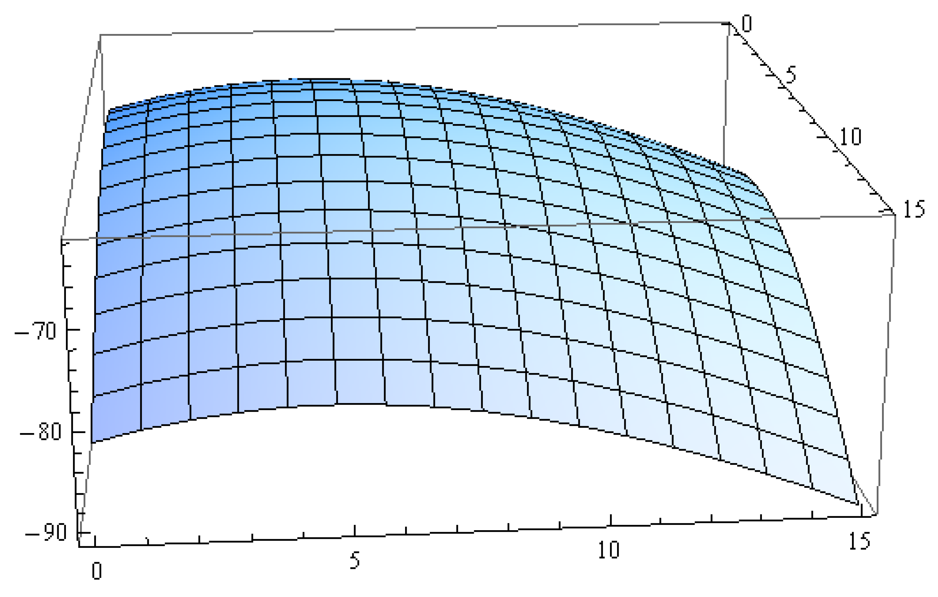
Using the joint Type-II GHCS presented by Table 6, we plotted the profile log-likelihood function (16) as in Figure 1. The maximum values need to begin with initial values of the parameters ${\beta }_1$ and ${\beta }_2$, showing that the iteration can be run with initial values that are almost in the neighborhood of the maximum values in Figure 1; therefore, the initial values were taken to be (${\beta }_1$, ${\beta }_2$) = (5, 6). 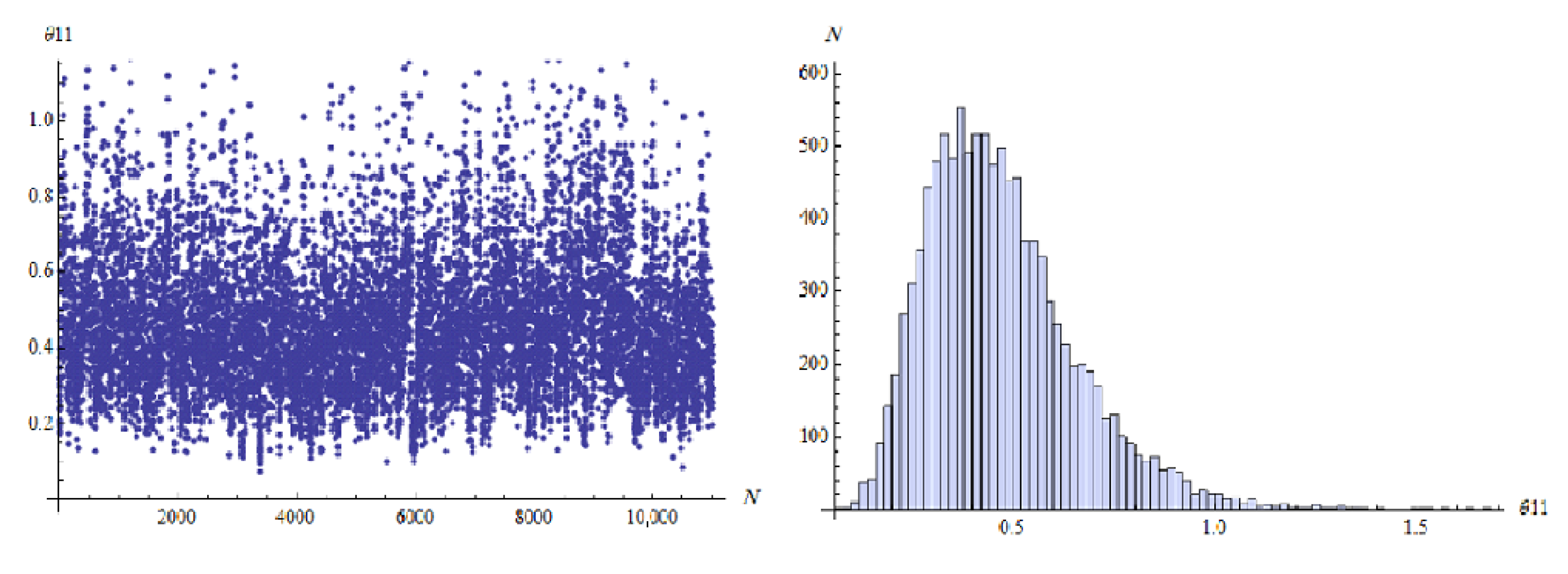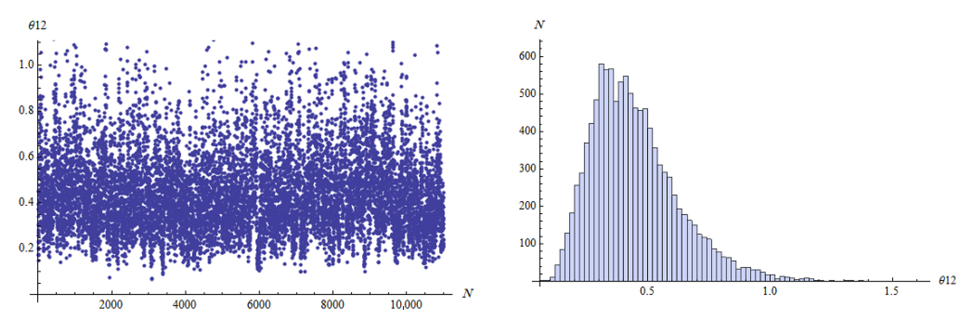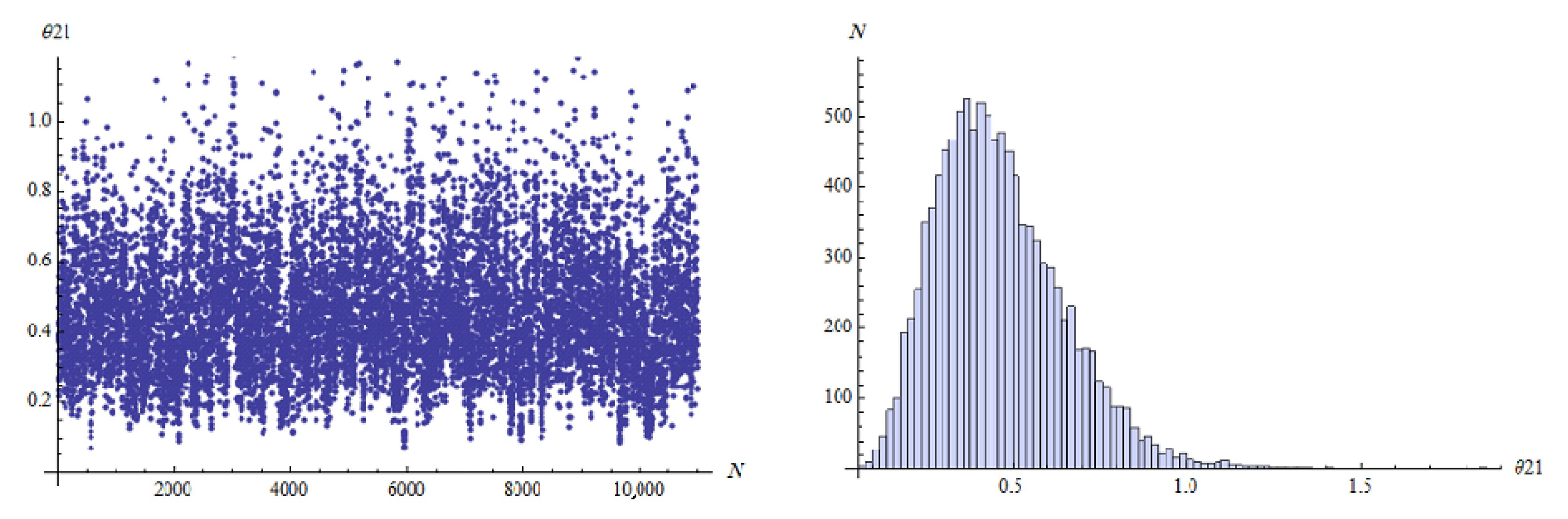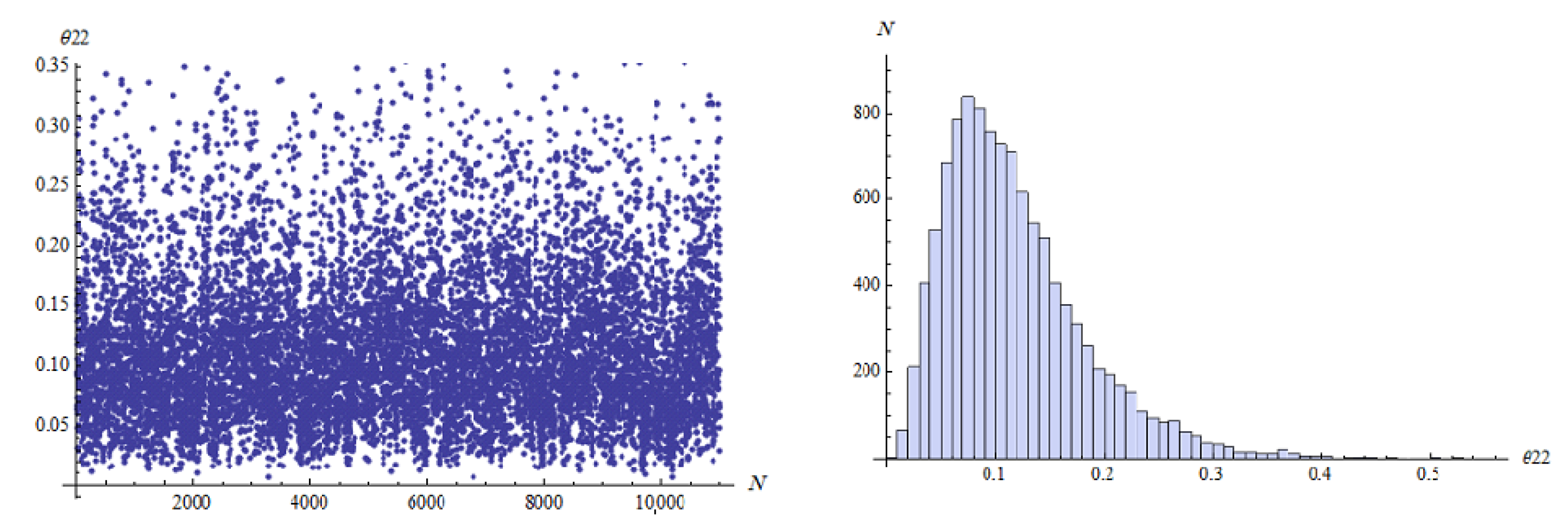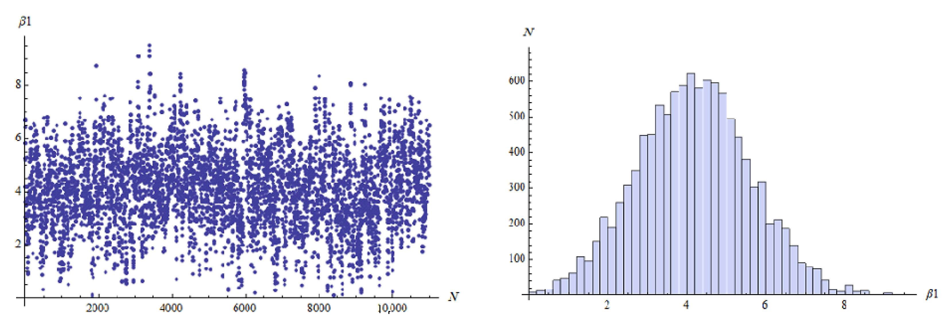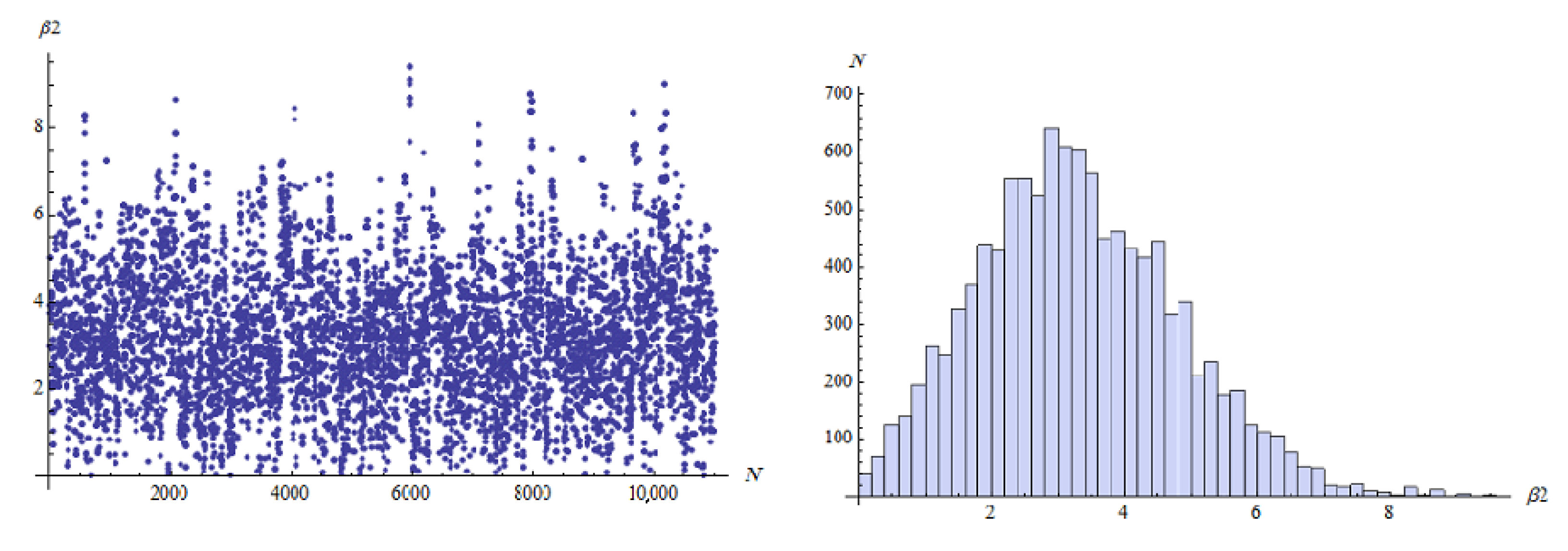For Bayes estimation, we adopted non-informative prior with $a_i=b_i=0.0001,$ $i=1,$ $2,$ …, 6. For the MCMC approach in Bayes method, we ran the chain 11,000 with the first 1000 values as burn-in. The MCMC approach that describes the empirical posterior distribution is shown in Figure 2, Figure 3, Figure 4, Figure 5, Figure 6 and Figure 7. Hence, the results of the ML point and interval estimates and different Bayes estimates were computed and the results are presented in Table 7 and

Table 8. Point estimates of the reliability and failure rates at $t=$ 0.1.

Method	${\mathit{R}}_{11}$	${\mathit{R}}_{12}$	${\mathit{R}}_{21}$	${\mathit{R}}_{22}$	${\mathit{h}}_{11}$	${\mathit{h}}_{12}$	${\mathit{h}}_{21}$	${\mathit{h}}_{22}$
(.)${}_{\mathrm{ML}}$	0.9569	0.9592	0.9609	0.9916	0.5654	0.5340	0.4963	0.1045
(.)${}_{\mathrm{Bayes}}$	0.9448	0.9475	0.9478	0.9864	0.6869	0.6523	0.6213	0.1588

.

9. Conclusions

Inference under various censoring techniques is crucial for life testing. Here, the problem of statistical inferences under a joint censoring scheme for Gompertz distribution is considered. Various inferences for unknown parameters of the proposed model were obtained from classical and Bayesian methods. We proposed that Gompertz units have two independent causes of failure, which can be determined using a competing risks model. Classical ML and bootstrap methods were used. Additionally, by using the Bayes technique and the MCMC method, the point and interval estimates were computed based on informative and non-informative priors. The asymptotic confidence intervals and Bayes credible intervals were also discussed. We used real data analysis and Monte Carlo simulation studies to assess and discuss the results. From the numerical result, we observed that the MLEs and non-informative Bayes estimations were closed. The Bayes method and bootstrap-t under informative prior P${}^1$ worked better than other methods. The numerical results generally showed that using an informative prior distribution in Bayes computations produces superior results to likelihood estimates. The estimates obtained under MCMC method also performed well for all sample sizes and affected sample size in terms of MSEs and interval average widths. The study demonstrated that the comparative Gompertz distributions has good flexibility for modeling joint samples of survival times of male mice under a conventional laboratory environment. Finally, we can say that the proposed model and proposed method of estimation work well. Therefore, our results are very important in the field of comparative life testing, especially when units fail due to several causes of failure.

References

1. Childs, A.; Chandrasekar, B.; Balakrishnan, N.; Kundu, D. Exact likelihood inference based on Type-I and Type-II hybrid censored samples from the exponential distribution. Ann. Inst. Stat. Math. 2003, 2, 319–330. [Google Scholar] [CrossRef]
2. Kundu, D.; Joarder, A. Analysis of type-II progressively hybrid censored data. Comput. Stat. Data Anal. 2006, 50, 2509–2528. [Google Scholar] [CrossRef]
3. Balakrishnan, N.; Rasouli, A.; Sanjari Farsipour, N. Exact likelihood inference based on an unified hybrid censored sample from the exponential distribution. J. Stat. Comput. Simul. 2008, 78, 475–488. [Google Scholar] [CrossRef]
4. Lone, S.A.; Panahi, H. Estimation procedures for partially accelerated life test model based on unified hybrid censored sample from the Gompertz distribution. Eksploat. Niezawodnosc-Maint. Reliab. 2022, 24, 427–436. [Google Scholar] [CrossRef]
5. Cox, D.R. The analysis of exponentially distributed lifetimes with two types of failures. J. R. Stat. Soc. 1959, 21, 411–421. [Google Scholar]
6. Crowder, M.J. Classical Competing Risks; Chapman and Hall: London, UK, 2001. [Google Scholar]
7. Balakrishnan, N.; Han, D. Exact inference for a simple step-stress model with competing risks for failure from exponential distribution under Type-II censoring. J. Stat. Plan. Inference 2008, 138, 4172–4186. [Google Scholar] [CrossRef]
8. Modhesh, A.A.; Abd-Elmougod, G.A. Analysis of Progressive First-Failure-Censoring in the Burr XII Model for Competing Risks Data. Am. J. Theor. Appl. Stat. 2015, 4, 610–618. [Google Scholar] [CrossRef] [Green Version]
9. Bakoban, R.A.; Abd-Elmougod, G.A. MCMC in analysis of progressively first failure censored competing risks data for Gompertz model. J. Comput. Theor. Nanosci. 2016, 10, 6662–6670. [Google Scholar] [CrossRef]
10. Debnath, P.; Mohiuddine, S.A. Soft Computing Techniques in Engineering, Health, Mathematical and Social Sciences; CRC Press: Boca Raton, FL, USA, 2021. [Google Scholar]
11. Alghamdi, A.S. Statistical inferences of competing risks generalized half-logistic lifetime populations in presence of generalized type-I hybrid censoring scheme. J. Comput. Theor. Nanosci. 2023, 65, 699–708. [Google Scholar] [CrossRef]
12. Ganguly, A.; Kundu, D. Analysis of simple step-stress model in presence of competing risks. J. Stat. Comput. Simul. 2016, 86, 1989–2006. [Google Scholar] [CrossRef]
13. Abu-Zinadah, H.H.; Neveen, S.A. Competing risks model with partially step-stress accelerate life tests in analyses lifetime Chen data under type-II censoring scheme. Open Phys. 2019, 17, 192–199. [Google Scholar] [CrossRef]
14. Rao, U.V.R.; Savage, I.R.; Sobel, M. Contributions to the theory of rank order statistics: The two-sample censored case. Ann. Math. Stat. 1960, 31, 415–426. [Google Scholar] [CrossRef]
15. Johnson, R.A.; Mehrotra, K.G. Locally most powerful rank tests for the two-sample problem with censored data. Ann. Math. Stat. 1972, 43, 823–831. [Google Scholar] [CrossRef]
16. Bhattacharyya, G.K.; Mehrotra, K.G. On testing equality of two exponential distributions under combined type-IIcensoring. J. Am. Stat. Assoc. 1981, 76, 886–894. [Google Scholar] [CrossRef]
17. Mehrotra, K.G.; Bhattacharyya, G.K. Confidence intervals with jointly type-II censored samples from two exponential distributions. J. Am. Stat. Assoc. 1982, 77, 441–446. [Google Scholar] [CrossRef]
18. Balakrishnan, N.; Rasouli, A. Exact likelihood inference for two exponential populations under joint type-II censoring. Comput. Stat. Data Anal. 2008, 52, 2725–2738. [Google Scholar] [CrossRef]
19. Rasouli, A.; Balakrishnan, N. Exact likelihood inference for two exponential populations under joint progressive type-II censoring. Commun. Stat. Theory Methods 2010, 39, 2172–2191. [Google Scholar] [CrossRef]
20. Shafaya, A.R.; Alakrishnanbc, B.N.; Abdel-Atyd, Y. Bayesian inference based on a jointly type-II censored sample from two exponential populations. J. Stat. Comput. Simul. 2014, 84, 2427–2440. [Google Scholar] [CrossRef]
21. Algarni, A.; Almarashi, A.M.; Abd-Elmougod, G.A.; Abo-Eleneen, Z.A. Two compound Rayleigh lifetime distributions in analyses the jointly type-II censoring samples. J. Math. Chem. 2019, 58, 950–966. [Google Scholar] [CrossRef]
22. Mondal, S.; Kundu, D. Bayesian Inference for Weibull Distribution under the Balanced Joint Type-II Progressive Censoring Scheme. Am. J. Math. Manag. Sci. 2019, 39, 56–74. [Google Scholar] [CrossRef]
23. Mondal, S.; Kundu, D. Inferences of Weibull parameters under balance two sample type-II progressive censoring scheme. Qual. Reliab. Eng. Int. 2020, 36, 1–17. [Google Scholar] [CrossRef]
24. Almarashi, A.M.; Algarni, A.; Daghistani, A.M.; Abd-Elmougod, G.A.; Abdel-Khalek, S.; Raqab, M.Z. Inferences for Joint Hybrid Progressive Censored Exponential Lifetimes under Competing Risk Model. Math. Probl. Eng. 2021, 2021, 3380467. [Google Scholar] [CrossRef]
25. Tahani, A.A.; Soliman, A.A.; Abd-Elmougod, G.A. Statistical inferences of Burr XII lifetime models under joint Type-1 competing risks samples. J. Math. 2021, 2021, 9553617. [Google Scholar]
26. Abdulaziz Alghamdi, S.; Abd-Elmougod, G.A.; Kundu, D.; Marin, M. Statistical Inference of Jointly Type-II Lifetime Samples under Weibull Competing Risks Models. Symmetry 2022, 14, 701. [Google Scholar] [CrossRef]
27. Soliman, A.A.; Abd Ellah, A.H.; Abou-Elheggag, N.A.; Abd-Elmougod, G.A. A simulation based approach to the study of coefficient of variation of Gompertz distribution under progressive first-failure censoring. Indian J. Pure Appl. Math. 2011, 42, 335–356. [Google Scholar] [CrossRef]
28. Soliman, A.A.; Abd Ellah, A.H.; Abou-Elheggag, N.A.; Abd-Elmougod, G.A. Estimation of the parameters of life for Gompertz distribution using progressive first-failure censoring data. Comput. Stat. Data Anal. 2012, 56, 2471–2485. [Google Scholar] [CrossRef]
29. Lodhi, C.; Tripathi, Y.M.; Bhattacharya, R. On a progressively censored competing risks data from Gompertz distribution. Commun. Stat. Simul. Comput. 2021, 56, 1–22. [Google Scholar] [CrossRef]
30. Wang, L.; Tripathi, Y.M.; Dey, S.; Shi, Y. Inference for dependence competing risks with partially observed failure causes from bivariate Gompertz distribution under generalized progressive hybrid censoring. Qual. Reliab. Eng. Int. 2021, 37, 1150–1172. [Google Scholar] [CrossRef]
31. Gupta, R.D.; Kundu, D. Hybrid censoring schemes with exponential failure distribution. Commun. Stat. Theory Methods 1998, 27, 3065–3083. [Google Scholar] [CrossRef]
32. Zhang, L.; Bhatti, M.M.; Michaelides, E.E.; Marin, M.; Ellahi, R. Hybrid nanofluid flow towards an elastic surface with tantalum and nickel nanoparticles, under the influence of an induced magnetic field. Eur. Phys. J. Spec. Top. 2022, 231, 521–533. [Google Scholar] [CrossRef]
33. Kundu, D.; Pradhan, B. Estimating the parameters of the generalized exponential distribution in presence of hybrid censoring. Commun. Stat. Theory Methods. 2009, 38, 2030–2041. [Google Scholar] [CrossRef] [Green Version]
34. Algarni, A.; Almarashi, M.A.; Abd-Elmougod, G.A. Joint type-I generalized hybrid censoring for estimation the two Weibull distributions. J. Inf. Sci. 2020, 36, 1243–1260. [Google Scholar]
35. Chandrasekar, B.; Childs, A.; Balakrishnan, N. Exact likelihood inference for the exponential distribution under generalized Type-I and Type-II hybrid censoring. Nav. Res. Logist. 2004, 51, 994–1004. [Google Scholar] [CrossRef]
36. Chakrabarty, J.B.; Chowdhury, S.; Roy, S. Optimum reliability acceptance sampling plan using Type-I generalized hybrid censoring scheme for products under warranty. Int. J. Qual. Reliab. Manag. 2019, 38, 780–799. [Google Scholar] [CrossRef]
37. Balakrishnan, N. Progressive censoring methodology: An appraisal. Test 2007, 16, 211–296. [Google Scholar] [CrossRef]
38. Balakrishnan, N.; Cramer, E. The Art of Progressive Censoring; Birkauser: New York, NY, USA, 2014. [Google Scholar]
39. El-Sherpieny, E.A.; Almetwally, E.M.; Muhammed, H.Z. Progressive Type-II Hybrid Censored Schemes based on Maximum Product Spacing with Application to Power Lomax Distribution. Physica A 2020, 553, 1–12. [Google Scholar] [CrossRef]
40. Abdul Mannan, M.; Rahman, M.R.; Akter, H.; Nahar, N.; Mondal, S. A Study of Banach Fixed Point Theorem and It’s Applications. Am. J. Comput. Math. 2021, 11, 157–174. [Google Scholar] [CrossRef]
41. Xu, J.; Long, J.S. Using the Delta Method to Construct Confidence Intervals for Predicted Probabilities, Rates, and Discrete Changes; Lecture Notes; Indiana University: Bloomington, IN, USA, 2005. [Google Scholar]
42. Wang, L.; Tripathi, Y.M.; Lodhi, C. Inference for Weibull competing risks model with partially observed failure causes under generalized progressive hybrid censoring. J. Comput. Appl. Math. 2020, 368, 1–15. [Google Scholar] [CrossRef]
43. Shih, J.H.; Emura, T. Likelihood-based inference for bivariate latent failure time models with competing risks under the generalized FGM copula. Comput. Stat. 2018, 33, 1293–1323. [Google Scholar] [CrossRef]
44. Davison, A.C.; Hinkley, D.V. Bootstrap Methods and Their Applications, 2nd ed.; Cambridge University Press: Cambridge, UK, 1997. [Google Scholar]
45. Efron, B.; Tibshirani, R.J. An Introduction to the Bootstrap; Chapman and Hall: New York, NY, USA, 1993. [Google Scholar]
46. Efron, B. The jackknife, the bootstrap and other resampling plans. In CBMS-NSF Regional Conference Series in Applied Mathematics; SIAM: Phiadelphia, PA, USA, 1982; Volume 38. [Google Scholar]
47. Hall, P. Theoretical comparison of bootstrap confidence intervals. Ann. Stat. 1988, 16, 927–953. [Google Scholar] [CrossRef]
48. Metropolis, N.; Rosenbluth, A.W.; Rosenbluth, M.N.; Teller, A.H.; Teller, E. Equations of state calculations by fast computing machines. J. Chem. Phys. 1953, 21, 1087–1091. [Google Scholar] [CrossRef] [Green Version]
49. Hoel, D.G. A Representation of Mortality Data by Competing Risks. Biometrics 1972, 28, 475–488. [Google Scholar] [CrossRef] [PubMed]
50. Pareek, B.; Kundu, D.; Kumar, S. On progressively censored competing risks data for Weibull distributions. Comput. Stat. Data Anal. 2009, 53, 4083–4094. [Google Scholar] [CrossRef]
51. Sarhan, A.M.; Hamilton, D.C.; Smith, B. Statistical analysis of competing risks models. Reliab. Eng. Syst. Saf. 2010, 95, 953–962. [Google Scholar] [CrossRef]
52. Cramer, E.; Schmiedt, A.B. Progressively Type-II censored competing risks data from Lomax distributions. Comput. Stat. Data Anal. 2011, 55, 1285–1303. [Google Scholar] [CrossRef]
Figure 1. Profile log-likelihood function (y-axis) of ( β 1 , x-axis) and ( β 2 , z-axis).
Axioms 12 00322 g001
Figure 2. Trace (Left) and histogram (Right) plots of the parameter θ 11 .
Axioms 12 00322 g002
Figure 3. Trace (Left) and histogram (Right) plots of the parameter θ 12 .
Axioms 12 00322 g003
Figure 4. Trace (Left) and histogram (Right) plots of the parameter θ 21 .
Axioms 12 00322 g004
Figure 5. Trace (Left) and histogram (Right) plots of the parameter θ 22 .
Axioms 12 00322 g005
Figure 6. Trace (Left) and histogram (Right) plots of the parameter β 1 .
Axioms 12 00322 g006
Figure 7. Trace (Left) and histogram (Right) plots of the parameter β 2 .
Axioms 12 00322 g007