
Renyi Entropy of the Residual Lifetime of a Reliability System at the System Level


1
Département de Mathématiques et d’Informatique, Université du Québec à Trois-Rivières, 3351 Boulevard des Forges, Trois-Rivières, QC G9A 5H7, Canada
2
Department of Statistics, United Arab Emirates University, Al Ain 15551, United Arab Emirates
3
Department of Statistics and Operations Research, College of Science, King Saud University, P.O. Box 2455, Riyadh 11451, Saudi Arabia
*
Author to whom correspondence should be addressed.
Axioms 2023, 12(4), 320; https://doi.org/10.3390/axioms12040320
Submission received: 5 February 2023
/
Revised: 18 March 2023
/
Accepted: 21 March 2023
/
Published: 23 March 2023
(This article belongs to the Special Issue Information Theory in Economics, Finance, and Management)
Abstract
:The measurement of uncertainty across the lifetimes of engineering systems has drawn more attention in recent years. It is a helpful metric for assessing how predictable a system’s lifetime is. In these circumstances, Renyi entropy, a Shannon entropy extension, is particularly appealing. In this paper, we develop the system signature to give an explicit formula for the Renyi entropy of the residual lifetime of a coherent system when all system components have lived to a time t. In addition, several findings are studied for the aforementioned entropy, including the bounds and order characteristics. It is possible to compare the residual lifespan predictability of two coherent systems with known signatures using the findings of this study.
MSC:
60E05; 62B10; 62N05; 94A171. Introduction
In physics, the idea of entropy has been crucial as a very useful measure. To indicate the thermodynamic change of heat that is transferred during the course of a reversible process at a specific temperature T, Clausius [1] invented the metric in 1850. However, entropy’s significance in statistical mechanics lies at a slightly deeper level, where it is typically viewed as the level of uncertainty in the state that a physical system can achieve or as a link between microscopic and macroscopic cases, since it calculates the number of states that an atom or molecule must take in order to satisfy a macroscopic configuration. Entropy’s application is not restricted to statistical analysis because it is directly related to the second law of thermodynamics and therefore applies to all other areas of physics. Entropy in statistical mechanics is measured using the Boltzmann–Gibbs measure, which is given by
in which stands as a discrete probability distribution on a random quantum state for N microstates. For , the measure H takes its greatest value (i.e., ), which holds when the state of system is in equilibrium. The Boltzmann–Gibbs entropy has the additivity property, as for two systems A and B which are non-interactive and adequately separated from each other with microstates and , respectively, which are accessible, one has . It is worth mentioning that H also has the extensity property (i.e., the composite system has an entropy which fulfills ). It should be noted that the entropy in Equation (1) does not depend on the dimension, so temperature in this discussion has the dimension of energy.
The application of entropy in mechanics, thermodynamics, and fatigue life modeling has been presented recently. For example, in the Basaran [2] theory, Newton’s universal laws of motion included the creation of an entropy. Lee et al. [3] used the thermodynamic state index (TSI) determined via cumulative entropy generation, which is used to predict the lifetime. On the basis of the theory used in unified mechanics, Lee et al. [4] introduced a fatigue life model to anticipate the fatigue life of metals at very high cycling using an entropy generation mechanism. Lee and Basaran [5] analyzed models based on an irreversible entropy as a metric with an empirical evolution function for empirical models developed in the context of Newtonian mechanics. Another fatigue model using entropy generation was proposed by Temfack and Basaran [6].
Several generalizations of the Boltzmann–Gibbs entropy have been brought forward to push the preparation of statistical mechanics to new limits. Several of these approaches have been prompted by the desire to maintain the thermodynamic limit while deforming the structured entropy of Equation (1) without free parameters (see, for example, the work of Obregón [7], Fuentes et al. [8], and Fuentes and Obregón [9]). Others have studied the relaxation of the measure in Equation (1) by introducing free parameters (see Kaniadakis [10] and Sharma and Mittal [11]). In the sequel to this paper, we will concentrate on the Renyi entropy (RE), which was first discussed in relation to coding and information theory by Renyi [12] as one of the first endeavors to extend the Shannon entropy (Shannon [13]). The definition of the RE is
where is a parameter that deforms the entropy structure. For example, if , then the RE corresponds to the Boltzmann–Gibbs case. The logarithmic structure allows the RE to retain the property of additivity no matter what value the parameter (which is free) takes, although the extensive property is no longer retained for any .
Because of its properties, the RE has gained considerable attention in information theory from both the quantum and classical perspectives (see, for example, the work of Campbell [14], Csiszar [15], and Goold et al. [16]). The RE is a powerful measure for quantizing quantum entanglement and the corresponding correlations which are strong, as they are found in a quantum field (Cui et al. [17]). For instance, in multipartite systems, the special case was discovered to be a measure of information describing the Gaussian states of harmonic quantum oscillators, resulting in strong inequalities of subadditivity that require generalized measures of mutual information (Adesso et al. [18]), the computation of which can be traced through path regularization schemes (Srdinšek [19]). Generalizations of conditional quantum information and the topological entanglement entropy are two more uses of the RE in quantum information (Berta et al. [20]). The RE has also been proposed as a method to describe phase changes between self-organized states in dynamical problems, both in complex systems (Beck [21] and Bashkirov [22]) and in fuzzy systems (Eslami-Giski et al. [23]), connected to the occurrence of quantum fuzzy trajectories (Fuentes [24]). This entropy measure’s viability has also been acknowledged in other disciplines, such as molecular imaging for therapeutic applications (Hughes [25]) and mathematical physics (Franchini et al. [26]) and biostatistics (Chavanis [27]). The concept of the RE can also be defined for a continuous distribution function (CDF) with some obvious modifications.
In the context of statistics and probability, quantifying uncertainties in a system’s lifetime is critical for engineers performing survival analysis. They concur that systems with higher dependability and longer lifetimes are better systems and that system reliability declines as uncertainties rise (see, for example, the work of Ebrahimi and Pellery [28]). Let X be a non-negative random variable (RV) with a probability density function (PDF) The RE, recognized as an RE of the order , is given by
in which “log” represents the natural logarithm. Specifically, the Shannon differential entropy [13] can be calculated as It is worth pointing out that the Shannon differential entropy is utilized to measure the uniformity of a PDF. In this case, the maximum entropy distribution is uniform. Hence, the values of which are greater induce more uncertainty being generated by the PDF f and, as a result, the ability to predict the next upshot of the RV
If X denotes the lifetime of a new system, then measures the uncertainty of the new system. In some cases, agents know something regarding the age of the system. For example, one may know that the system is alive at time t and is interested in the uncertainty, the value it takes, and its RL (i.e., ). Then, will not be useful in such situations. Accordingly, the residual RE is
where
is the PDF of , is the survival function (SF) of X, and is the quantile function of . Various properties, generalizations, and applications of were investigated by Asadi et al. [29], Gupta and Nanda [30], Nanda and Paul [31], and the authors of the references therein.
We recall that a number of standards are available for assessing the aging process of a lifetime unit. To this aim, the residual lifetime (RL) will be, in turn, an illustrative measure of the aging behavior. In fact, in a situation where the distribution of the RL is not affected by the age of a system, it is said that this is a no-aging aspect of the system. Thus, the behavior of the RL is considered dominant when one studies the aging phenomenon in a component or, more generally, in a system. In this paper, the RE of the RL of a system is evaluated. Namely, a formula for the RE of the RL is presented whenever the components of the system are working at time t. The expressions are based on system signatures, lifetime distribution functions, and the beta distribution. The concept of a system signature is used when the lifetimes the components of a coherent system have are independent and identically distributed (IID). Ebrahimi [32] initiated the concept of the dynamic Shannon entropy and acquired several aspects this measure has. Toomaj and Doostparat [33] studied the classic Shannon entropy and its possessions for mixed systems, and moreover, further findings on the measure have also been achieved (see also [34]). Recently, Toomaj et al. [35] investigated some results concerning the information aspects in working systems in use by applying a dynamic signature. In this paper, we continue this line of research and investigate some results on the RE properties of working used systems using system signatures. In fact, we generalize the results of the aforementioned papers.
The results of this work are organized as follows. In Section 2, we provide an expression for the RE of a coherent system under the assumption that all components have survived to a certain point in time. The residual RE is also ordered based on some ordering properties of system signatures without being computed directly in Section 3. Section 4 presents some useful limits and bounds for the new measure. There are some remarks that may be useful in future studies, which are given in Section 5.
In the remaining parts of the paper, the notations “”, “”, “”, and “” are used to signify the usual stochastic order, the hazard rate order, the likelihood ratio order, and the dispersive order, respectively. For the further aspects and properties these orders have, the reader can be referred to Shaked and Shanthikumar [36].
2. Renyi Entropy of the Residual Lifetime
In this section, we use the concept of the system signature to find an assertion for the RE of the RL of a system with a coherent structure that has an arbitrary system-level structure in the sense that we know that the components contained in the system are all in operation at a time t. The signature a coherent system having n components has is an n-dimensional vector for which the jth element , in which T represents the lifetime the underlying coherent system has and represent the order statistics of n IID lifetimes of the components with an unchanged distribution. For more details, see, for example, the work of Samaniego [37]. Let us think about a coherent structure with IID component lifetimes and a known signature vector . If represents the RL of the system provided that, at time all components of the system are functioning, then from the results of Khaledi and Shaked [38], the SF of is derivable as follows:
where denotes the RL of an i-out-of-n system, provided that the components are all operating at the time t. The SF and PDF of are given by
and
respectively, where is the complete gamma function. It follows that
In what follows, we will concentrate on the study of the RE of the RV , which measures the degree of uncertainty induced by the PDF of with respect to the predictability of the RL of the system in terms of the RE. The transformation plays a crucial role in our goal. It is clear that follows from a beta distribution having the parameters and i with the PDF
Next, we give a statement on the RE of by applying the earlier transformations:
Theorem 1.
The RE of can be derived as
where for all
Proof.
In the last equality, is the PDF of V, which signifies the lifetime the system with the IID uniform distribution has. □
According to Equation (11), if (standing for the signature of an i-out-of-n system), then
in which follows the beta distribution having the parameters and and
such that stands for the beta function. In the special case for , Equation (12) coincides with the results of Abbasnejad and Arghami [39].
The next theorem follows directly from Theorem 1, concerning the aging properties of its components. We recall that X has an increasing (decreasing) failure rate (IFR (DFR)) if in x is decreasing (increasing) for all :
Theorem 2.
If X is the IFR (DFR), then is decreasing (increasing) in t for all .
Proof.
We just prove this for when X is the IFR, while the proof for the DFR is similar. It is plain to observe that This implies that Equation (11) can be rewritten as
for all Instead, one can find that for all and hence one has
If , then . Therefore, when F is the IFR, then for all we have
for all Using (14), we get
for all This implies that for all , and this completes the proof. □
The next example illustrates the results of Theorems 1 and 2:
Example 1.
Contemplate a bridge system with a system signature The exact value of can be calculated using the relation in Equation (11), given the distributions of component lifetimes. For this purpose, let us assume the following lifetime distributions:
- (i)
- We see that is decreasing in We note that the uniform distribution has the IFR property, and therefore decreases as t increases, as we expected based on Theorem 2.
- (ii)
- Think about a Pareto type II with the SFIt is not hard to see thatIt is obvious that the RE of is increasing in terms of Thus, the uncertainty of the conditional lifetime increases as t increases. We recall that this distribution has the DFR property.
- (iii)
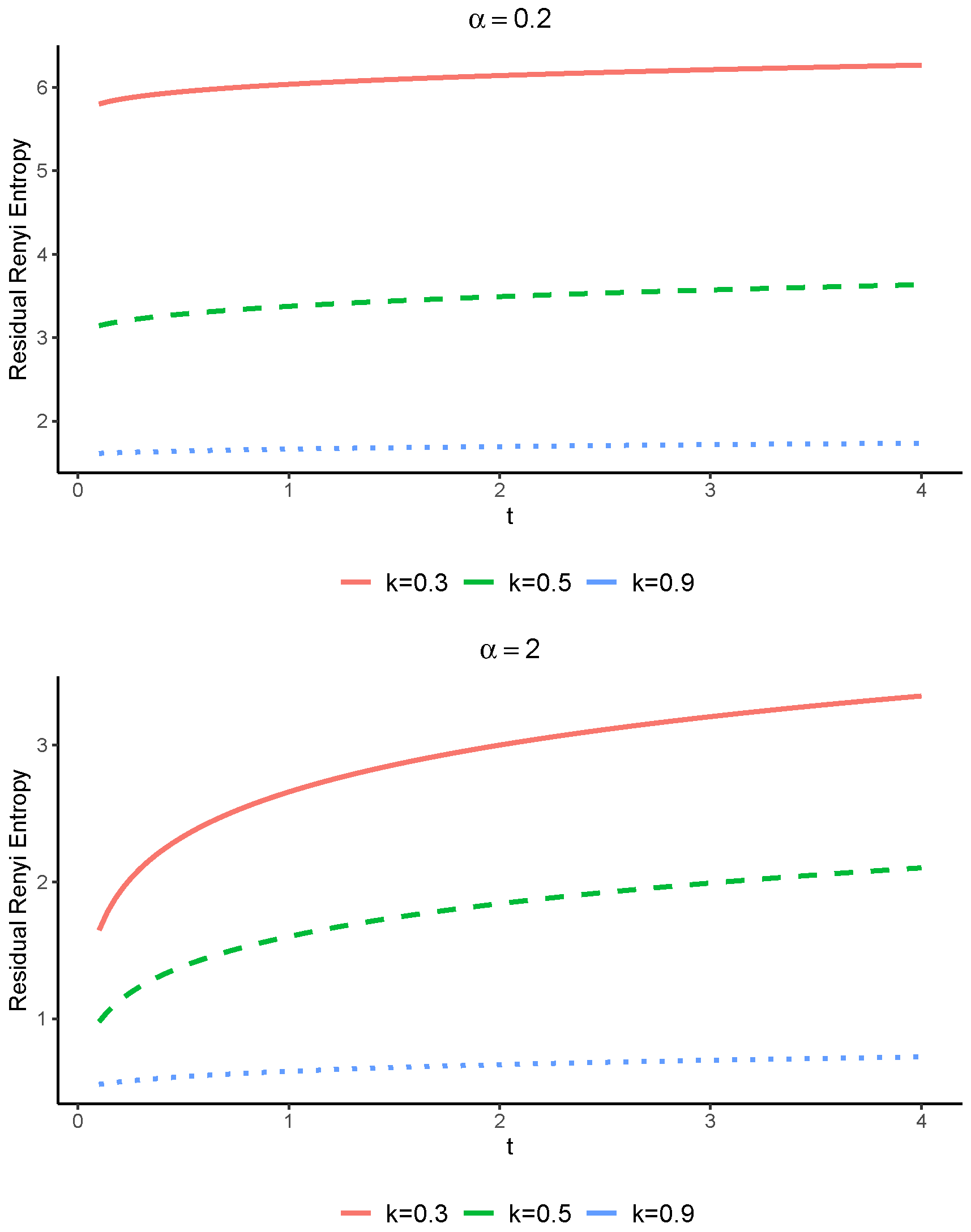
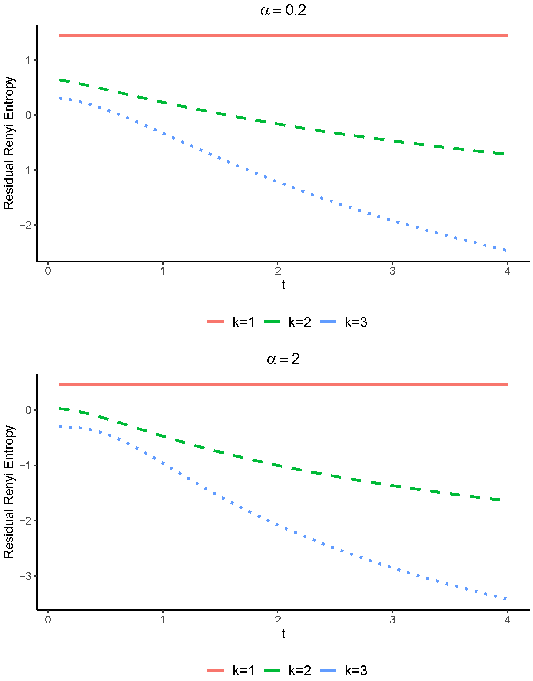
- Let us suppose that X has a Weibull distribution with the shape parameter k and with the SFThrough some manipulation, we obtainIt is not a facile assignment to acquire a plain statement for the above relation, and therefore we computed it numerically. In Figure 1, we framed the entropy of in terms of the time t for values of and as well as , which has the DFR property. As expected from Theorem 2, it is evident that increases in In Figure 2, we plotted the entropy of with respect to time t for values of and along with , which has the IFR property. As expected from Theorem 2, it is evident that decreases in
Below, we compare the Renyi entropies of two coherent system lifetimes and their residual lifetimes.
Theorem 3.
Consider a coherent system with IID IFR (DFR) component lifetimes. Then, for all .
Proof.
We prove the theorem for the case when X is the IFR, where the proof for the DFR property is similar. Since X is the IFR, Theorem 3.B.25 of Shaked and Shanthikumar [36] implies that ; that is, we have
for all If then we have
Therefore, the proof is completed. □
We remark that Theorem 3 reveals that when the lifetimes the components have are the IFR (DFR), then the RE of the working coherent system when all components of the system are alive at time t are less (greater) than the RE of the new system. The next theorem provides a lower bound for the residual RE in terms of the RE of the new system:
Theorem 4.
If X is the DFR, then a lower bound for is given as follows:
for all
Proof.
Since X is the DFR, then it is NWU (i.e., ). This implies that
for all On the other hand, if X is the DFR, then the PDF f is decreasing, which implies that
for all From Equation (11), one can conclude that
for all and this completes the proof. □
3. Renyi Entropy Comparison
In this section, we are concerned with the partial ordering (that is, it has reflexive, transitive, and antisymmetric properties) of the conditionally represented lifetimes in two coherent systems on the basis of their uncertainties. We report a number of achievements for making orderings between two coherent systems on the basis of different existing orderings among the lifetimes their components have and the associated vectors of the signature. In the next result, we analyze the entropies of the residual lifetimes of two coherent systems with the same structures:
Theorem 5.
Let and denote the RLs of two coherent systems with matching signatures and n IID component lifetimes and from CDFs F and G, respectively. If , and X or Y is the IFR, then for all
Proof.
Example 2.
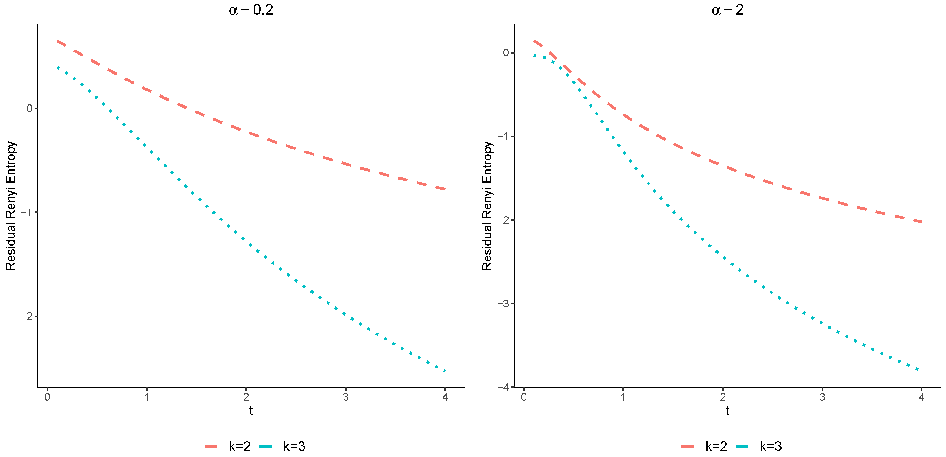
Let us assume two coherent systems with residual lifetimes and with the common signature Suppose that and , where stands for the Weibull distribution with the SF given in Equation (17). It is easy to see that Moreover, X and Y are both the IFR. Therefore, Theorem 5 yields that for all The plots of the Renyi entropies of these systems are displayed in Figure 3.
In the next result, we analyze the residual REs for two coherent systems having matching component lifetimes and distinct structures:
Theorem 6.
Let and signify the RLs of two coherent systems with vectors of signatures given by and , respectively. Suppose that the system’s components are IID according to the CDF F, and also also let Then, we have the following:
- (i)
- If increases in u for all then for all .
- (ii)
- If decreases in u for all then for all .
Proof.
Assumption implies , and this gives that , which means that
increases in u for all , and hence When we obtain
where the inequality in Equation (20) is obtained by noting that the conditions imply for all increasing (decreasing) functions Therefore, the relation in Equation (19) gives
or equivalently, for all Part (ii) can be obtained in a similar way. □
The next example gives an application of Theorem 6:
Example 3.
Let and be the signatures of two coherent systems of the order , with residual lifetimes and Let us consider a Pareto type II with the SF given in Equation (16). After some calculation, one can find
Clearly, the above function is increasing in u for all (i.e., increases in u for all ). Hence, due to Theorem 6, it holds that for all .
4. Bounds for the Renyi Entropy of the Residual Lifetime
When the distributions of the component lifetimes are not precisely known, or when the component number and the complexity of the system are high, it is not plain to work out for a coherent system. This situation is frequently encountered in practice. A residual RE bound can be useful to be close to the behavior of the lifetime of a coherent system under such circumstances. Toomaj and Doostparast [33,34] obtained bounds on the entropy a coherent system induces through its lifetime for a new system. Recently, Toomaj et al. [35] obtained some bounds for the entropy of the coherent system under the assumption that the components contained in the system were all alive. In the following theorem, we provide bounds on the residual RE of the lifetime of the coherent system in terms of the residual RE of the parent distribution :
Theorem 7.
Let represent the RL of a coherent system consisting of n IID component lifetimes with a common CDF F that has the signature . Let for all It holds that
for , where and
Proof.
It is easy to see that the mode the beta distribution having the parameters and i has is Therefore, we obtain
Thus, for we have
The last equality is obtained from Equation (5), which the desired result follows. □
The bounds in Equation (21) are quite helpful when the component number is extensive or the configuration the system induces is difficult. Now, a lower bound is acquired from the properties of the RE measure:
Theorem 8.
Underneath the requirements of Theorem 7, we have
where for all
Proof.
The Jensen’s inequality as it applies to the function (which is concave (convex) for ) yields
Thus, we obtain
The inequality given above is followed by the linearity of the integration operator. Since , then by multiplying both sides in Equation (24) in , the intended result is achieved. □
We note that the inequality in Equation (23) is satisfied for i-out-of-n systems in the sense that for and for , while . As the lower bounds for in both assertions of Theorems 7 and 8 can be evaluated, we can use the maximum value the lower bounds take:
Example 4.
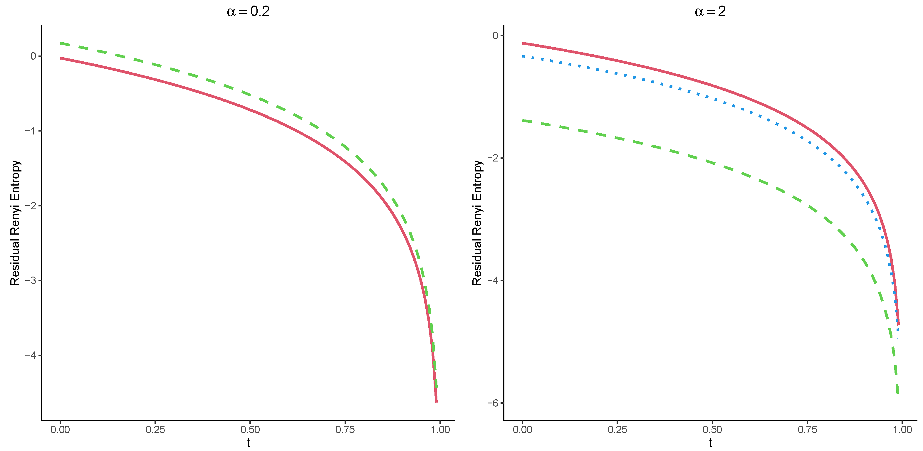
Let signify the RL of a coherent system with the signature and with IID component lifetimes uniformly distributed over It is easy to verify that Thus, under Theorem 7, the RE of takes some bounds for as shown below:
Moreover, the lower bound given in Equation (23) can be obtained as follows:
for all For the component lifetimes, assumed to be uniformly distributed, the bounds given in Equation (25) (dashed line) are calculated, and the exact value is obtained from (11) while the bounds are derived in Equation (26) (dotted line). The results are displayed in Figure 4. As we can see, the lower bound in Equation (26) (dotted line) for is better than the lower bound given by Equation (25).
5. Conclusions
Clearly, any system that is in operation longer and has less uncertainty about its remaining lifetime is a better system because it makes more accurate predictions. This fact makes it obvious that system uncertainty is a prestigious aspect of systems in engineering. To this end, a useful criterion is to measure the predictability of the lifetime of a system by using the RE as an extension of the Shannon entropy. In this work, we found a simple statement for the uncertainty the lifetime of a system induces under the assumption that all system components are functioning at time t (t can be the age of a system) with regard to the RE. Several stochastic properties of the proposed measure were also discussed. Some limits were presented and some partial order behaviors fulfilled by the RLs of two coherent systems on the basis of their REs being studied appealing to the concept of the signature of a system. The results were examined in some examples to illustrate the concepts presented in this paper. In reliability engineering, there are more complex systems that include coherent systems whose lifetimes are given in terms of successive failure times of the components assembled to form the system. To make clear what the contribution of the authors in this work is, it is worth mentioning that the properties of the Shannon differential entropy of the work systems used have been studied in the literature (see, for example, the work of Toomaj et al. [35]). However, since the Renyi entropy is a generalization of the Shannon differential entropy, and we used it in our study, we used the earlier extended results of Toomaj et al. [35], which from this perspective can be considered the novelty of our work. We feel that the results of the present work contain more information about the information properties of functioning systems than in the case of the application of the Shannon differential entropy. Moreover, the novel bound given in Theorem 7 in Section 4 is straightforward and easy to compute since it depends on the known beta distribution.
In future work, we can focus on the RE properties of such systems to provide a new framework and open a new window to the predictability of the lifetime a coherent system has from a novel perspective.
Author Contributions
Conceptualization, M.M.; methodology, M.M.; software, M.K.; validation, M.M.; formal analysis, M.K.; investigation, M.M.; resources, M.S.; writing—original draft preparation, M.M.; writing—review and editing, M.K.; visualization, M.S.; supervision, M.S.; project administration, M.S.; funding acquisition, M.S. All authors have read and agreed to the published version of the manuscript.
Funding
The first author was funded by the Natural Sciences and Engineering Research Council of Canada (No. 06536-2018). The research of the second and third authors was funded by Researchers Supporting Project number (RSP2023R464) of King Saud University in Riyadh, Saudi Arabia.
Informed Consent Statement
Not applicable.
Data Availability Statement
No new data were created or analyzed in this study. Data sharing is not applicable to this article.
Acknowledgments
The authors are thankful to three anonymous reviewers for their constructive comments. The first author acknowledges financial support from the Natural Sciences and Engineering Research Council of Canada (No. 06536-2018). The second and third authors acknowledge financial support from the Researchers Supporting Project number (RSP2023R464), King Saud University, Riyadh, Saudi Arabia.
Conflicts of Interest
The authors declare no conflict of interest.
References
- Clausius, R. The Mechanical Theory of Heat; MacMillan and Co.: London, UK, 1879. [Google Scholar]
- Basaran, C. Introduction to Unified Mechanics Theory with Applications; Springer Nature: Berlin/Heidelberg, Germany, 2023. [Google Scholar]
- Lee, H.W.; Fakhri, H.; Ranade, R.; Basaran, C.; Egner, H.; Lipski, A.; Piotrowski, M.; Mroziński, S. Modeling fatigue of pre-corroded body-centered cubic metals with unified mechanics theory. Mater. Des. 2022, 224, 111383. [Google Scholar] [CrossRef]
- Lee, H.W.; Basaran, C.; Egner, H.; Lipski, A.; Piotrowski, M.; Mroziński, S.; Rao, C.L. Modeling ultrasonic vibration fatigue with unified mechanics theory. Int. J. Solids Struct. 2022, 236, 111313. [Google Scholar] [CrossRef]
- Lee, H.W.; Basaran, C. A review of damage, void evolution, and fatigue life prediction models. Metals 2021, 11, 609. [Google Scholar] [CrossRef]
- Temfack, T.; Basaran, C. Experimental verification of thermodynamic fatigue life prediction model using entropy as damage metric. Mater. Sci. Technol. 2015, 31, 1627–1632. [Google Scholar] [CrossRef]
- Obregón, O. Superstatistics and gravitation. Entropy 2010, 12, 2067. [Google Scholar] [CrossRef] [Green Version]
- Fuentes, J.; López, J.L.; Obregón, O. Generalized Fokker-Planck equations derived from nonextensive entropies asymptotically equivalent to Boltzmann-Gibbs. Phys. Rev. E 2020, 102, 012118. [Google Scholar] [CrossRef]
- Fuentes, J.; Obregón, O. Optimisation of information processes using non-extensive entropies without parameters. Int. J. Inf. Coding Theory 2022, 6, 35–51. [Google Scholar] [CrossRef]
- Kaniadakis, G.; Lissia, M.; Rapisarda, A. Non Extensive Thermodynamics and Its Applications; Springer Science & Business Media: Berlin/Heidelberg, Germany, 2002; Volume 305, pp. 1–305. [Google Scholar]
- Sharma, B.; Mittal, D. New nonadditive measures of entropy for discrete probability distributions. J. Math. Sci. 1975, 10, 28–40. [Google Scholar]
- Rényi, A. On Measures of Information and Entropy. In Proceedings of the Fourth Berkeley Symposium on Mathematical Statistics and Probability, Berkeley, CA, USA, 20 June–30 July 1960; pp. 547–561. [Google Scholar]
- Shannon, C.E. A mathematical theory of communication. Bell Syst. Tech. 1948, 27, 379–423. [Google Scholar] [CrossRef] [Green Version]
- Campbell, L. A coding theorem and Rényi’s entropy. Inf. Control 1965, 8, 423–425. [Google Scholar] [CrossRef] [Green Version]
- Csiszar, I. Generalized cutoff rates and Rényi’s information measures. IEEE Trans. Inf. Theory 1995, 41, 26–34. [Google Scholar] [CrossRef]
- Goold, J.; Huber, M.; Riera, A.; Rio, L.D.; Skrzypczyk, P. The role of quantum information in thermodynamics—A topical review. J. Phys. A Math. Theor. 2016, 49, 1–34. [Google Scholar] [CrossRef]
- Cui, J.; Gu, M.; Kwek, L.C.; Santos, M.F.; Fan, H.; Vedral, V. Quantum phases with differing computational power. Nat. Commun. 2012, 3, 812. [Google Scholar] [CrossRef] [Green Version]
- Adesso, G.; Girolami, D.; Serafini, A. Measuring Gaussian Quantum Information and Correlations Using the Rényi Entropy of Order 2. Phys. Rev. Lett. 2012, 109, 190502. [Google Scholar] [CrossRef] [Green Version]
- Srdinšek, M.; Casula, M.; Vuilleumier, R. Quantum Rényi entropy by optimal thermodynamic integration paths. Phys. Rev. Res. 2022, 4, L032002. [Google Scholar] [CrossRef]
- Berta, M.; Seshadreesan, K.P.; Wilde, M.M. Rényi generalizations of quantum information measures. Phys. Rev. A 2015, 91, 022333. [Google Scholar] [CrossRef] [Green Version]
- Beck, C. Upper and lower bounds on the Renyi dimensions and the uniformity of multifractals. Phys. D Nonlinear Phenom. 1990, 41, 67–78. [Google Scholar] [CrossRef]
- Bashkirov, A.G. Rényi entropy as a statistical entropy for complex systems. Theor. Math. Phys. 2006, 149, 1559–1573. [Google Scholar] [CrossRef]
- Eslami-Giski, Z.; Ebrahimzadeh, A.; Markechová, D. Rényi entropy of fuzzy dynamical systems. Chaos Solitons Fractals 2019, 123, 244–253. [Google Scholar] [CrossRef]
- Fuentes, J. Quantum control operations with fuzzy evolution trajectories based on polyharmonic magnetic fields. Sci. Rep. 2020, 10, 22256. [Google Scholar] [CrossRef]
- Hughes, M.S.; Marsh, J.N.; Arbeit, J.M.; Neumann, R.G.; Fuhrhop, R.W.; Wallace, K.D.; Thomas, L.; Smith, J.; Agyem, K.; Lanza, G.M.; et al. Application of Rényi entropy for ultrasonic molecular imaging. J. Acoust. Soc. Am. 2009, 125, 3141–3145. [Google Scholar] [CrossRef] [PubMed] [Green Version]
- Franchini, F.; Its, A.R.; Korepin, V.E. Renyi entropy of the XY spin chain. J. Phys. A Math. Theor. 2007, 41, 025302. [Google Scholar] [CrossRef]
- Chavanis, P.H. Nonlinear mean field Fokker-Planck equations. Application to the chemotaxis of biological populations. Eur. Phys. J. B 2008, 62, 179–208. [Google Scholar] [CrossRef] [Green Version]
- Ebrahimi, N.; Pellerey, F. New partial ordering of survival functions based on the notion of uncertainty. J. Appl. Probab. 1995, 32, 202–211. [Google Scholar] [CrossRef]
- Asadi, M.; Ebrahimi, N.; Soofi, E.S. Dynamic generalized information measures. Stat. Probab. Lett. 2005, 71, 85–98. [Google Scholar] [CrossRef]
- Gupta, R.D.; Nanda, A.K. K-and L-entropies and relative entropies of distributions. J. Stat. Theory Appl. 2002, 1, 177–190. [Google Scholar]
- Nanda, A.K.; Paul, P. Some results on generalized residual entropy. Inf. Sci. 2006, 176, 27–47. [Google Scholar] [CrossRef]
- Ebrahimi, N. How to measure uncertainty in the residual life time distribution. Sankhyā Indian J. Stat. Ser. A 1996, 58, 48–56. [Google Scholar]
- Toomaj, A.; Doostparast, M. A note on signature-based expressions for the entropy of mixed r-out-of-n systems. Nav. Res. Logist. 2014, 61, 202–206. [Google Scholar] [CrossRef]
- Toomaj, A. Renyi entropy properties of mixed systems. Commun. Stat.-Theory Methods 2017, 46, 906–916. [Google Scholar] [CrossRef]
- Toomaj, A.; Chahkandi, M.; Balakrishnan, N. On the information properties of working used systems using dynamic signature. Appl. Stoch. Model. Bus. Ind. 2021, 37, 318–341. [Google Scholar] [CrossRef]
- Shaked, M.; Shanthikumar, J.G. Stochastic Orders; Springer Science and Business Media: New York, NY, USA, 2007. [Google Scholar]
- Samaniego, F.J. System Signatures and Their Applications in Engineering Reliability; Springer Science and Business Media: Berlin/Heidelberg, Germany, 2007; Volume 110. [Google Scholar]
- Khaledi, B.-E.; Shaked, M. Ordering conditional lifetimes of coherent systems. J. Stat. Plan. Inference 2007, 137, 1173–1184. [Google Scholar] [CrossRef]
- Abbasnejad, M.; Arghami, N.R. Renyi entropy properties of order statistics. Commun. Stat.-Theory Methods 2010, 40, 40–52. [Google Scholar] [CrossRef]
- Ebrahimi, N.; Kirmani, S.N.U.A. Some results on ordering of survival functions through uncertainty. Stat. Probab. Lett. 1996, 29, 167–176. [Google Scholar] [CrossRef]
Figure 1.
The exact values of with respect to t for the Weibull distribution for values of and when .
Figure 1.
The exact values of with respect to t for the Weibull distribution for values of and when .

Figure 2.
The exact values of with respect to t for the Weibull distribution for values of and when .
Figure 2.
The exact values of with respect to t for the Weibull distribution for values of and when .

Figure 3.
The exact values of (blue color) and (red color) with respect to t for values of and .


Disclaimer/Publisher’s Note: The statements, opinions and data contained in all publications are solely those of the individual author(s) and contributor(s) and not of MDPI and/or the editor(s). MDPI and/or the editor(s) disclaim responsibility for any injury to people or property resulting from any ideas, methods, instructions or products referred to in the content. |
© 2023 by the authors. Licensee MDPI, Basel, Switzerland. This article is an open access article distributed under the terms and conditions of the Creative Commons Attribution (CC BY) license (https://creativecommons.org/licenses/by/4.0/).
Share and Cite
MDPI and ACS Style
Mesfioui, M.; Kayid, M.; Shrahili, M. Renyi Entropy of the Residual Lifetime of a Reliability System at the System Level. Axioms 2023, 12, 320. https://doi.org/10.3390/axioms12040320
AMA Style
Mesfioui M, Kayid M, Shrahili M. Renyi Entropy of the Residual Lifetime of a Reliability System at the System Level. Axioms. 2023; 12(4):320. https://doi.org/10.3390/axioms12040320
Chicago/Turabian StyleMesfioui, Mhamed, Mohamed Kayid, and Mansour Shrahili. 2023. "Renyi Entropy of the Residual Lifetime of a Reliability System at the System Level" Axioms 12, no. 4: 320. https://doi.org/10.3390/axioms12040320
Note that from the first issue of 2016, this journal uses article numbers instead of page numbers. See further details here.