Article

A Numerical Implementation of Fractional-Order PID Controllers for Autonomous Vehicles

1
Department of Mathematics, Al Zaytoonah University of Jordan, Amman 11733, Jordan
2
Nonlinear Dynamics Research Center (NDRC), Ajman University, Ajman P.O. Box 346, United Arab Emirates
3
Department of Mathematics, Zarqa University, Zarqa 11831, Jordan
4
Department of Mathematics, Prince Sattam Bin Abdulaziz University, Alkharj 11942, Saudi Arabia
5
Department of Mathematics, Faculty of Science, University of Jordan, Amman 11942, Jordan
*
Author to whom correspondence should be addressed.
Axioms 2023, 12(3), 306; https://doi.org/10.3390/axioms12030306
Submission received: 15 January 2023 / Revised: 15 February 2023 / Accepted: 22 February 2023 / Published: 17 March 2023
(This article belongs to the Special Issue Control Theory and Its Application in Mathematical Biology)

Abstract

:
In the context of reaching the best way to control the movement of autonomous cars linearly and angularly, making them more stable and balanced on different roads and ensuring that they avoid road obstacles, this manuscript chiefly aims to reach the optimal approach for a fractional-order PID controller (or P I γ D ρ -controller) instead of the already classical one used to provide smooth automatic parking for electrical autonomous cars. The fractional-order P I γ D ρ -controller is based on the particle swarm optimization (PSO) algorithm for its design, with two different approximations: Oustaloup’s approximation and the continued fractional expansion (CFE) approximation. Our approaches to the fractional-order PID using the results of the PSO algorithm are compared with the classical PID that was designed using the results of the Cohen–Coon, Ziegler–Nichols and bacteria foraging algorithms. The scheme represented by the proposed P I γ D ρ -controller can provide the system of the autonomous vehicle with more stable results than that of the PID controller.

1. Introduction

Recently, the subject of self-driving systems has taken up a large part of the research into car development. In order for these systems to work in an effective manner, the car must have a number of sensors to collect information about traffic, the surrounding areas of the car and pedestrians, as well as information on traffic safety under different climatic conditions.
In self-driving cars, research and practical experiments have been aimed at developing the PID controller, which is latent in the heart of the autonomous car, into a highly accurate sensor that provides quick and stable responses. Such a controller is typically used to determine the deviation of the car’s position, the position of the axle, the balance of the four rotors and independent cars that are following a certain path smoothly without overtaking [1,2,3,4,5,6].
The PID controller has a wide range of applications in many industrial fields due to its effectiveness in controlling systems [7,8]. Most notably, flow and temperature measurement systems, cars and engines of all kinds. The PID controller is built from an integro-differential equation whose simplicity lies in the adjustment of three different parameters: k p , k i and k d . By optimizing these parameters, the improvement in device performance is more obvious and precise. Among the most widely used PID-controller tuning methods in control engineering are the Ziegler–Nichols and Cohen–Coon methods, the particle swarm optimization algorithm, the bacteria foraging algorithm, the genetic algorithm, the artificial bee colony, ant colony optimization, the grey wolf optimizer, the hybrid optimization technique and many others [9]. The Cohen–Coon tuning method is the second most popular after the Zeigler–Nichols tuning method because it is more flexible than the Zeigler–Nichols tuning method in a wider variety of processes. The Cohen–Coon tuning method is reasonable for processes where the dead time is less than twice that of the time constant, but the Zeigler–Nichols tuning method works well only on processes where the dead time is less than half that of the time response [10]. In the same regard, the particle swarm optimization (PSO) technique, proposed by Kennedy and Eberhart [11], is an evolutionary-type global optimization technique, whose development was inspired by social activities in flock of birds and schools of fish, and it is widely applied to various engineering problems due to its high computational efficiency. Compared with other population-based stochastic optimization methods, such as the genetic algorithm, PSO has a comparable or even superior search performance for many hard optimization problems, with faster and more stable convergence rates. It has been proved to be an effective optimum tool in system identification and PID-controller tuning for a class of processes [12]. The efficiency of, e.g., the genetic algorithm can be used to create an objective function that evaluates the PID gains based on the overall errors of the systems and generate a high quality solution [13].
Recently, the PID controller has been improved using the concept of fractional calculus [14]. With this new concept, the PID controller has been upgraded from the classic PID controller to a fractional-order PID controller. According to this concept, the equation from the classical controller was updated into the fractional-order PID controller [14]. Based on this evolution, the further tuning of two parameters, the fractional-order integral value ( γ ) and the fractional-order derivative value ( ρ ) , in addition to the three existing ones, are needed. These two parameters require proper handling of the fractional-order Laplacian operators, s γ and s ρ , which can be approximated by different numerical approaches, such as the continued fractional expansion (CFE) scheme, Oustaloup’s approximation and others. These approximations are characterized by the ability to convert the fractional-order Laplacian operators, ( s γ and s ρ ) , into their corresponding integer-order rational transfer functions. In general, these techniques can improve the PID controller by transforming it into the P I γ D ρ -controller by optimizing the five parameters ( K p , K i , K d , γ , ρ ) .
In this manuscript, we are interested in implementing the PSO optimization algorithm for the purpose of tuning the fractional-order PID controller in order to make the control system for self-driving cars on different roads and situations more stable, more controlled and more responsive. The CFE and Oustaloup approaches were used to approximate the fractional-order Laplacian operators, s γ and s ρ . Our approaches to fractional-order PID using the results of the PSO algorithm were compared with the classical PID controller that was designed using the results of the Cohen–Coon (CC) approach, the Ziegler–Nichols (ZN) method and the bacteria foraging algorithm (BFA).
In this work, we emphasize the fact that the fractional-order PID controller can provide better results over standard PID controllers, here by proposing different P I γ D ρ -controllers for autonomous vehicle systems that were established based on the application of the PSO algorithm simultaneously with the use of two different approximations (Oustaloup and the continued fractional expansion) of the fractional-order integro-differential Laplacian operators. Actually, including these two approaches within the autonomous vehicle system, using the PSO algorithm to verify the validity of using the fractional-order PID controller, is regarded as the main contribution of this work.

2. The Fractional-Order PID Controller

Podlubny et al. are credited with creating the fractional-order PID controller in 1977 by adding two extra parameters ( γ and ρ ) to the basic parameters ( K p , K i , K d ) of the PID controller, which clearly shows the high response speed of this construction compared to the classical version [15,16,17]. Generally, the PID controller is obtained by using the following fractional-order integro-differential equation [18]:
y ( t ) = K p e ( t ) + K i J γ e ( t ) + K d D ρ e ( t ) ,
where J γ is the Riemann–Liouville operator of order γ , D ρ is the Caputo operator of order ρ and e ( t ) is the error signal. By utilizing the forward Laplace transform of (1), we obtain the following:
Z ( s ) = Y ( s ) E ( s ) = K p + K i s γ + K d s ρ ,
where E ( s ) = L ( e ( t ) ) is the Laplace transform of e ( t ) .
The main objective of this work was to effectively enable the provided controller inside autonomous electric vehicles to provide a safe and stable place away from road hazards for the autonomous vehicle. Accordingly, the PSO algorithm [11,14,19,20] was applied to obtain the best values for the five parameters of the fractional-order PID controller. The parameters of the PSO algorithm used throughout this work are taken as shown in Table 1.
As for optimality theory, building the so-called fitness function within the algorithm and reducing its value was the ultimate goal of this theory, through which it is easy to obtain the optimal values for the fractional-order PID controller. According to what has been mentioned, we are in the process of adopting a specific fitness function [19,20]. The following is how such a fitness function (integral time absolute error (ITAE)) can be expressed:
V = 0 t | e t | d t ,
where e ( t ) is the error signal over the time t. However, the overall tuning process of the PID controller using the PSO algorithm can be described by the block diagram shown in Figure 1.
To obtain the optimal tuning of a given system, it is necessary to approximate the fractional-order Laplacian operators: s γ and s ρ . This can be performed specifically by using the CFE and Oustaloup approaches, which are based on the development of two appropriate equations for the above-mentioned Laplacian operators; however, the reader can obtain more comprehensive information about these two approaches by referring to the following content.

2.1. The CFE Approximation

This method is regarded as the primary mathematical approach for providing the Laplacian operator by proper integer-order rational transfer functions. Such an approach was established based on the following approximation [21]:
( 1 + z ) α = 1 1 α z 1 + ( 1 + α ) z 2 + ( 1 α ) z 3 ( 2 + α ) z 2 + ( 2 α ) z 5 + + ( n + α ) z 2 + ( n α ) z 2 n + 1 + ,
where 0 < α < 1 and n N .
For the purpose of obtaining a finite-order approximation of the operator s α , one might replace the term s for the variable z in (4). This exchange step enables the nth-order approximation of such operators to appear around the center frequency ω 0 = 1 rad / s , as follows [21]:
s α α 0 s n + α 1 s n 1 + + α n 1 s + α n α n s n + α n 1 s n 1 + + α 1 s + α 0 ,
where 0 < α i < 1 , i = 0 , 1 , 2 , , 5 . In particular, the coefficient values of α i can be found in reference [21], for i = 0 , 1 , , 5 . Moreover, the operator s α can be simply obtained by inverting the expression given in (5).

2.2. Oustaloup’s Approximation

Oustaloup’s approximation is a popular approximation that can be used to generate specific rational transfer functions of odd-order only. The bandwidth over which the approximation is considered can be customized to yield a good fitting to the fractional-order elements s ± α within a predefined frequency band, where 0 < α < 1 . Thus, for geometrically distributed frequencies over the frequency range of interest ( ω b , ω h ) , the following rational function is used for approximating s α [22]:
s α k = N N s + ω k s + ω k = B n s n + B n 1 s n 1 + + B 1 s + B 0 A n s n + A n 1 s n 1 + + A 1 s + A 0 ,
where the poles, zeros and the gain are evaluated form the following relations:
ω k = ω b ω h ω b K + N + 0.5 ( 1 + α ) 2 N + 1 ,
ω k = ω b ω h ω b K + N + 0.5 ( 1 α ) 2 N + 1 ,
K = ω h ω b α 2 K = N N ω K ω k .
Due to the geometrical distribution of frequencies, the unity-gain geometric frequency ω u is calculated from the following:
ω u = ω b . ω h ,
where the approximation depends on the order filer N and the lower frequency range ( ω b , ω h ) .
Observe that the order of the transfer function (6) is always of order n = 2 N + 1 . In the special case where the limited frequencies ω b and ω h are symmetrical around the center frequency, ω u = 1 rad / s , (i.e., ω b = 1 / ω h ), then the coefficients of (6) will be correlated to each other as follows [22]:
A n i = B i , i = 0 , 1 , 2 , , N .

3. The Design of the Fractional-Order PID Controller for Autonomous Cars

Regarding the execution of system data, the system was initially programmed using MATLAB by giving it the system inputs and executing it to obtain the required output. The MATLAB code implements the two tuning methods mentioned for the fractional-order PID controller in autonomous cars, analyzes them and then obtains and evaluates the results. In fact, the system is described with two different types of transfer function for modeling the steering, which is represented by a servo motor, and the car motion, which is represented by DC motors. By defining the system for each of the linear motion subsystems and the angular motion subsystem, the results were obtained as in [23]. The input to the linear motion subsystem is the voltage, and the output is the velocity. For the angular motion subsystem, the voltage is also the input, and the output is the angular velocity. The angular motion, which has two poles with no zeros, is given as the following transfer function [23]:
T 1 ( s ) = 0.121 s 2 + 0.619 s + 0.1636 .
In addition, the transfer function of the linear motion, which has two poles with no zeros, can be formulated as follows [23]:
T 2 ( s ) = 0.008936 s 2 + 0.1258 s + 0.02384 .
From this point of view, we aim to reduce the fitness function given in (3) by using the PSO algorithm followed by approximating the resulting fractional-order operators ( s γ and s ρ ) using the CFE and Oustaloup methods. Through these approximations, we obtained two fractional-order PID controllers C i ( s ) , which necessarily means we also obtained two closed-loop systems H i ( s ) , where i = 1 , 2 . We compared all closed-loop systems to derive the best controller for the proposed subsystems.
In the following two subsections, different results of the proposed improvements are shown, and the results of the CC, ZN and BFA improvements for the classic PID controller are listed and compared by specific graphics and tables. The preferences of the proposed novel improvements is also shown.

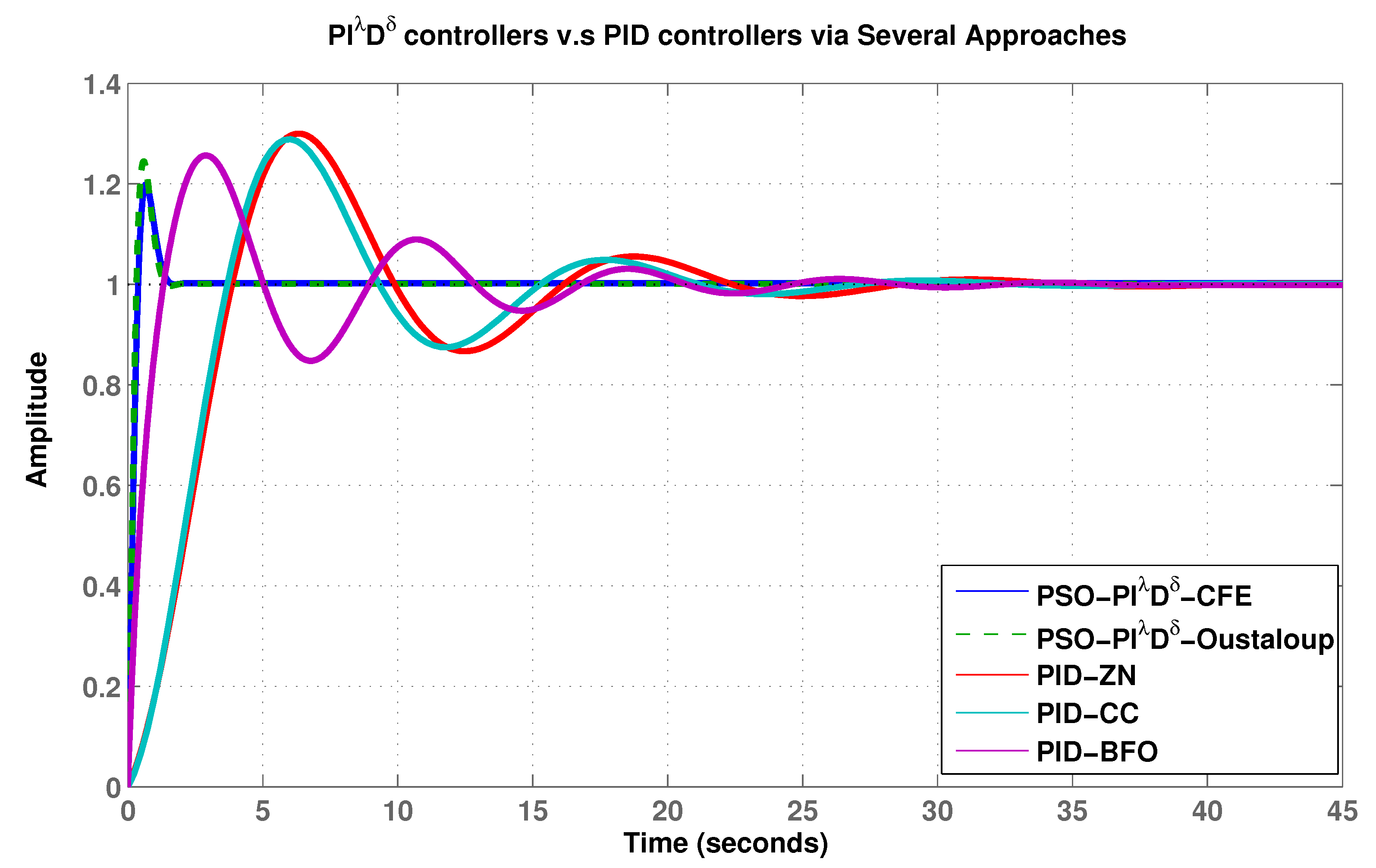
3.1. Tuning Fractional-Order PID of Linear Transfer Motion

In this part, we execute the PSO algorithm to obtain two fractional-order PID controllers, C 1 ( s ) and C 2 ( s ) , to tune the linear transfer motion T 2 ( s ) given in (13). These controllers are given as follows:
  • The P I γ D ρ -PSO-controller via the CFE approach:
C 1 ( s ) = 14.7631 + 0.31 s 0.911 + 51 s 0.867 .
Using the CFE approach turns the two operators, s 0.911 and s 0.8670 , into the following integer-order rational transfer functions:
s 0.911 = 2.4696 e + 2 s 5 + 2.6421 e + 3 s 4 + 5.607 e + 3 s 3 + 2.9951 e + 3 s 2 + 3.3208 e + 2 s + 0.9999 s 5 + 3.32084 e + 2 s 4 + 2.9951 e + 3 s 3 + 5.6074 e + 3 s 2 + 2.6421 e + 3 s + 2.4696 e + 2
and
s 0.867 = 1.4201 e + 2 s 5 + 1.5719 e + 3 s 4 + 3.4354 e + 3 s 3 + 1.8949 e + 3 s 2 + 2.2056 e + 2 s + 1 s 5 + 2.2056 e + 2 s 4 + 1.8949 e + 3 s 3 + 3.4354 e + 3 s 2 + 1.5719 e + 3 s + 1.42014 e + 2 ,
where e here is shorthand for × 10 ( · ) . Therefore, C 1 ( s ) in (14) is transformed into the following form:
C 1 ( s ) = 1.792 e 6 s 10 + 3.978 e 7 s 9 + 3.113 e 8 s 8 + 1.063 e 9 s 7 + 1.792 e 9 s 6 + 1.561 e 9 s 5 + 7.168 e 8 s 4 + 1.702 e 8 s 3 + 1.982 e 7 s 2 + 9.843 e 5 s + 1.302 e 4 247 s 10 + 5.711 e 4 s 9 + 1.056 e 6 s 8 + 7.095 e 6 s 7 + 2.075 e 7 s 6 + 2.92 e 7 s 5 + 2.011 e 7 s 4 + 6.647 e 6 s 3 + 9.508 e 5 s 2 + 4.873 e 4 s + 142 .
This consequently yields the following closed-loop system:
H 1 ( s ) = 2.594 e 7 s 10 + 5.75 e 8 s 9 + 4.505 e 9 s 8 + 1.538 e 10 s 7 + 2.593 e 10 s 6 + 2.259 e 10 s 5 + 1.037 e 10 s 4 + 2.463 e 9 s 3 + 2.868 e 8 s 2 + 1.424 e 7 s + 1.884 e 5 247 s 13 + 7.599 e 4 s 12 + 5.448 e 6 s 11 + 1.2 e 8 s 10 + 1.255 e 9 s 9 + 6.899 e 9 s 8 + 1.992 e 10 s 7 + 3.068 e 10 s 6 + 2.531 e 10 s 5 + 1.118 e 10 s 4 + 2.572 e 9 s 3 + 2.923 e 8 s 2 + 1.427 e 7 s + 1.884 e 5 .
  • The P I γ D ρ -PSO-controller via Oustaloup’s approach:
C 2 ( s ) = 0.17 + 9.88342 s 0.2823 + 61 s 0.976 .
In this case, we use Oustaloup’s approach to approximate the two operators, s 0.2823 and s 0.976 , which are in the following two forms:
s 0.2823 = 3.66 s 5 + 133.8 s 4 + 667.5 s 3 + 514.6 s 2 + 61.35 s + 1 s 5 + 61.35 s 4 + 514.6 s 3 + 667.5 s 2 + 133.8 s + 3.669
and
s 0.976 = 89.54 s 5 + 1724 s 4 + 4538 s 3 + 1847 s 2 + 116.2 s + 1 s 5 + 116.2 s 4 + 1847 s 3 + 4538 s 2 + 1724 s + 89.54 .
Actually, the above two Laplacian operators can convert (19) into the following form:
C 2 ( s ) = 2.005 e 4 s 10 + 1.119 e 6 s 9 + 1.883 e 7 s 8 + 1.123 e 8 s 7 + 2.676 e 8 s 6 + 2.622 e 8 s 5 + 1.216 e 8 s 4 + 2.898 e 7 s 3 + 3.641 e 6 s 2 + 1.93 e 5 s + 3323 3.669 s 10 + 560.1 s 9 + 2.299 e 4 s 8 + 3.419 e 5 s 7 + 1.906 s 6 + 4.218 e 6 s 5 + 3.611 e 6 s 4 + 1.227 e 6 s 3 + 1.564 e 5 s 2 + 7217 s + 89.54 .
Hence, the corresponding closed-loop system is in the following form:
H 2 ( s ) = 2.901 e 5 s 10 + 1.619 e 7 s 9 + 2.725 e 8 s 8 + 1.625 e 9 s 7 + 3.872 e 9 s 6 + 3.795 e 9 s 5 + 1.76 e 9 s 4 + 4.194 e 8 s 3 + 5.268 e 7 s 2 + 2.793 e 6 s + 4.809 e 4 3.669 s 13 + 840.6 s 12 + 6.621 e 4 s 11 + 2.451 e 6 s 10 + 4.674 e 7 s 9 + 4.599 e 8 s 8 + 2.16 e 9 s 7 + 4.613 e 9 s 6 + 4.286 e 9 s 5 + 1.907 e 9 s 4 + 4.373 e 8 s 3 + 5.35 e 7 s 2 + 2.803 e 6 s + 4.81 e 4 .
  • The PID controller via the bacteria-foraging-algorithm (BFA) approach: herein, we implement the BFA to obtain the PID controller. The output form is as follows:
C 3 = 12.7302 + 14.0836 s + 22.4950 s ,
which immediately gives the closed-loop system H 3 ( s ) , which has the form:
H 3 ( s ) = 325.5 s 2 + 184.2 s + 203.8 s 4 + 76.43 s 3 + 435.3 s 2 + 184.3 s + 203.8 .
  • The PID controller via the Ziegler–Nichols (ZN) approach: herein, we implement the ZN algorithm to obtain the PID controller. The output is of the following form:
C 4 ( s ) = 2.5 + 0.582 / s + 4.271 s .
This, consequently, implies the closed-loop system H 4 ( s ) , which is in the following form:
H 4 ( s ) = 61.81 s 2 + 36.18 s + 8.422 s 4 + 0.7306 s 3 + 171.6 s 2 + 36.31 s + 8.422 .
  • The PID controller via the Cohen-Coon (CC) approach: here, we applied the CC algorithm to obtain the PID controller. This controller has the following form:
C 5 ( s ) = 3.02 + 0.472 / s + 2.81 s .
Therefore, the closed-loop system H 5 ( s ) is expected to be as follows:
H 5 ( s ) = 40.66 s 2 + 43.7 s + 6.83 s 4 + 76.43 s 3 + 150.4 s 2 + 43.83 s + 6.83 .
Table 2 presents a numerical comparison between the five methods in which the gain of PID and FOPID is shown based on a certain transfer function of linear motion. Table 3 draws attention to the dynamic results of the closed-loop transfer functions given in H 1 , H 2 , H 3 , H 4 and H 5 , while Figure 2 reflects the advantage and accuracy of the CFE and Oustaloup methods as they show a clear decrease in the amount of overshoot followed by a tendency to quickly stabilize.

3.2. Tuning the Fractional-Order PID Controller for Angular Transfer Motion

Similarly to the previous subsection, we re-execute the PSO algorithm once again, but this time to obtain two other fractional-order PID controllers C 6 ( s ) and C 7 ( s ) . This tunes the angular transfer motion T 1 ( s ) given in (12). These controllers are given as follows:
  • The P I γ D ρ -PSO-controller via the CFE approach:
C 6 ( s ) = 48 + 24.2411 s 0.911 + 51 s 0.7119 .
The two Laplacian operators, s 0.911 and s 0.7119 , can, therefore, be approximated using the CFE approach as follows:
s 0.911 = 2.4696 e + 2 s 5 + 2.6421 e + 3 s 4 + 5.6074 e + 3 s 3 + 2.9951 e + 3 s 2 + 3.3208 e + 2 s + 0.9999 s 5 + 3.32 . 084 e + 2 s 4 + 2.9951 e + 3 s 3 + 5.6074 e + 3 s 2 + 2.6421 e + 3 s + 2.4696 + 2
and
s 0.7119 = 38.7389 s 5 + 4.8518 e + 2 s 4 + 1.1765 e + 3 s 3 + 7.2524 e + 2 s 2 + 99.1305 s + 1 s 5 + 99.1305 s 4 + 7.2524 e + 2 s 3 + 1.1765 e + 3 s 2 + 4.8518 e + 2 s + 38.7389 .
Thus, the P I γ D ρ -controller C 6 ( s ) is of the form:
C 6 ( s ) = 4.998 e 5 s 10 + 1.264 e 7 s 9 + 31.136 e 8 s 8 + 4.583 e 8 s 7 + 9.503 e 8 s 6 + 1.087 e 9 s 5 + 7.179 e 8 s 4 + 2.752 e 8 s 3 + 5.861 e 7 s 2 + 6.048 e 6 s + 2.338 e 5 247 s 10 + 2.712 e 4 s 9 + 4.466 e 5 s 8 + 2.766 e 6 s 7 + 7.592 e 6 s 6 + 1.009 e 7 s 5 + 6.588 e 6 s 4 + 2.062 e 6 s 3 + 2.783 e 5 s 2 + 1.335 e 4 s 38.74 .
This, consequently, implies the closed-loop system H 6 ( s ) , which is in the following form:
H 6 ( s ) = 6.047 e 4 s 10 + 1.53 e 6 s 9 + 1.375 e 7 s 8 + 5.545 e 7 s 7 + 1.15 e 8 s 6 + 1.316 e 8 s 5 + 8.687 e 7 s 4 + 3.33 e 7 s 3 + 7.092 e 6 s 2 + 7.319 e 5 s + 2.829 e 4 247 s 12 + 2.728 e 4 s 11 + 5.239 e 5 s 10 + 4.576 e 6 s 9 + 2.312 e 7 s 8 + 7.07 e 7 s 7 + 1.291 e 8 s 6 + 1.394 e 8 s 5 + 8.95 e 7 s 4 + 3.38278 s 3 + 7.146 e 6 s 2 + 7.341 e 5 s + 2.83 e 4 .
  • The P I γ D ρ -PSO-controller via Oustaloup’s approach:
C 7 ( s ) = 59 + 61.8823 s 0.821 + 61 s 0.7167 .
The two operators, s 0.821 and s 0.7167 , can be approximated using Oustaloup’s approach as follows:
s 0.821 = 43.85 s 5 + 973.9 s 4 + 2957 s 3 + 1388 s 2 + 100.8 s + 1 s 5 + 100.8 s 4 + 1388 s 3 + 2957 s 2 + 973.9 s + 43.85
and
s 0.7167 = 27.13 s 5 + 663.2 s 4 + 2217 s 3 + 1146 s 2 + 91.53 s + 1 s 5 + 91.53 s 4 + 1146 s 3 + 2217 s 2 + 6373.2 s + 27.13 .
This allows (35) to be rewritten in the following form:
C 7 ( s ) = 7.522 e 4 s 10 + 3.692 e 6 s 9 + 5.935 e 7 s 8 + 3.597 e 8 s 7 + 9.902 e 8 s 6 + 1.333 e 9 s 5 + 9.65 e 8 s 4 + 3.478 e 8 s 3 + 5.796 e 7 s 2 + 3.647 e 6 s + 7.528 e 4 43.85 s 10 + 4987 s 9 + 1.424 e 5 s 8 + 1.485 e 6 s 7 + 5.704 e 6 s 6 + 8.803 e 6 s 5 + 5.18 e 6 s 4 + 1.225 e 6 s 3 + 106724 s 2 + 3398 s + 27.13 .
Hence, the closed-loop system is in the following form:
H 7 ( s ) = 9101 s 10 + 4.467 e 5 s 9 + 7.181 e 6 s 8 + 4.352 e 7 s 7 + 1.198 e 8 s 6 + 1.613 e 8 s 5 + 1.168 e 8 s 4 + 4.209 e 7 s 3 + 7.014 e 6 s 2 + 4.413 e 5 s + 9109 43.85 s 12 + 5015 s 11 + 1.545 e 5 s 10 + 2.021 e 6 s 9 + 1.383 e 7 s 8 + 5.61 e 7 s 7 + 1.314 e 8 s 6 + 1.672 e 8 s 5 + 1.185 e 8 s 4 + 4.236 e 7 s 3 + 7.033 e 6 s 2 + 4.418 e 5 s + 9113 .
  • The PID controller via the bacteria foraging algorithm (BFA): in this part, we obtain the following result:
C 8 ( s ) = 8.4629 + 10.5707 s + 13.1024 s .
This leads to the following closed-loop system:
H 8 ( s ) = 1.585 s 2 + 1.024 s + 1.279 s 3 + 2.204 s 2 + 1.188 s + 1.279 .
  • The PID controller via the Ziegler–Nichols (ZN) approach: in this part, we have the following:
C 9 ( s ) = 1.94 + 1.02 s + 0.9922 s .
This, consequently, implies the closed-loop system H 9 ( s ) , which is of the following form:
H 9 ( s ) = 0.1116 s 2 + 0.2347 s + 0.1234 s 3 + 0.7306 s 2 + 0.3983 s + 0.1234 .
  • The PID controller via the Cohen–Coon (CC) approach: herein, we have
C 10 ( s ) = 2.22 + 1.01 s + 0.745 s .
This gives the closed-loop system H 8 ( s ) , which is of the following form:
H 10 ( s ) = 0.09015 s 2 + 0.2686 s + 0.1222 s 3 + 0.7091 s 2 + 0.4322 s + 0.1222 .
Regarding angular movement motion, Table 4 shows the gains of the fractional-order PID controllers for each method, Table 5 shows their dynamic results and, finally, Figure 3 shows the effect of applying the different methods on the fractional-order PID controller and the greater stability of the CFE and Oustaloup methods.

4. Conclusions

In order to obtain the best performance of passenger car movement and stability on and off the roads, along with higher flexibility on straight and angular roads according to changing conditions and safety from sudden obstacles that appear on the roads, different control units have been designed. In particular, different P I γ D ρ -controllers were established based on the application of the PSO algorithm simultaneously with the use of two different approximations of the fractional-order integro-differential Laplacian operators. These approximations are Oustaloup’s approximation and the continued fractional expansion (CFE) approximation. Based on the numerical results gained from several performed comparisons, we conclude that there are significant improvements in the step responses achieved by using P I γ D ρ -controllers over using PID controllers. In particular, in order not to obtain too much overshoot, we can implement the best controller among all of the proposed controllers, which is the P I γ D ρ -controller that was established by executing the PSO algorithm through the CFE approach. On the other hand, in order to obtain the fastest step response and fastest settling time, one may choose the P I γ D ρ -controller, which was established by executing the PSO algorithm through Oustaloup’s approach. In general, the P I γ D ρ -controller provides an autonomous vehicle with more stable results than that of the PID controller.

Author Contributions

Conceptualization, I.M.B. and A.A.A.-N.; Data curation, I.M.B. and S.A.; Formal analysis, I.M.B., O.Y.A. and A.A.A.-N.; Funding acquisition, W.G.A., S.A., S.M. and O.Y.A.; Investigation, S.A.; Methodology, I.M.B. and A.A.A.-N.; Project administration, W.G.A. and S.M.; Resources, S.A., O.Y.A. and S.M.; Software, O.Y.A.; Supervision, S.A. and S.M.; Validation, O.Y.A.; Visualization, S.M.; Writing—original draft, S.A.; Writing—review & editing, S.A. All authors have read and agreed to the published version of the manuscript.

Funding

This research received no external funding.

Data Availability Statement

Not applicable.

Conflicts of Interest

The authors declare no conflict of interest.

References

  1. Ammar, H.H.; Azar, A.T. Robust path tracking of mobile robot using fractional order pid controller. In Advances in Intelligent Systems and Computing, Proceedings of the International Conference on Advanced Machine Learning Technologies and Applications (AMLTA2019), Cairo, Egypt, 28–30 March 2019; Hassanien, A.E., Azar, A.T., Gaber, T., Bhatnagar, R.F., Tolba, M., Eds.; Springer International Publishing: Cham, Switzerland, 2020; pp. 370–381. [Google Scholar]
  2. Ammar, H.H.; Azar, A.T.; Tembi, T.D.; Tony, K.; Sosa, A. Design and implementation of fuzzy PID controller into multi agent smart library system prototype. In Advances in Intelligent Systems and Computing, Proceedings of the International Conference on Advanced Machine Learning Technologies and Applications (AMLTA2018), Cairo, Egypt, 22–24 February 2018; Hassanien, A.E., Tolba, M.F., Elhoseny, M., Mostafa, M., Eds.; Springer International Publishing: Cham, Switzerland, 2018; pp. 127–137. [Google Scholar]
  3. Azar, A.T.; Serrano, F.E. Design and Modeling of Anti Wind up PID Controllers; Springer International Publishing: Cham, Switzerland, 2015; pp. 1–44. [Google Scholar]
  4. Azar, A.T.; Vaidyanathan, S. Handboook of Research on Advanced Intelligent Control Engineering and Automation; IGI Global: New York, NY, USA, 2015. [Google Scholar]
  5. Bimbraw, K. Autonomous cars: Past, present and future a review of the developments in the last century, the present scenario and the expected future of autonomous vehicle technology. In Proceedings of the 2015 12th International Conference on Informatics in Control, Automation and Robotics (ICINCO), Colmar, France, 21–23 July 2015; Volume 1, pp. 191–198. [Google Scholar]
  6. Ogata, K. Modern Control Engineering; Prentice Hall: Upper Saddle River, NJ, USA, 2010. [Google Scholar]
  7. Jeongheon, H.; Skelton, R. An LMI optimization approach for structured linear controllers. In Proceedings of the 42nd IEEE International Conference on Decision and Control, Maui, HI, USA, 9–12 December 2003; pp. 5143–5148. [Google Scholar]
  8. Kalangadan, A.; Priya, N.; Kumar, T.K.S. PI, PID controller design for interval systems using frequency response model matching technique. In Proceedings of the International Conference on Control, Communication and Computing India, ICCC 2015, Trivandrum, India, 19–21 November 2015; pp. 119–124. [Google Scholar]
  9. Ahmmed, T.; Akhter, I.; Karim, S.M.R.; Sabbir Ahamed, F.A. Genetic Algorithm Based PID Parameter Optimization. Am. J. Intell. Syst. 2020, 10, 8–13. [Google Scholar] [CrossRef]
  10. Suksawat, T.; Kaewpradit, P. Comparison of Ziegler-Nichols and Cohen-Coon Tuning Methods: Implementation to Water Level Control Based MATLAB and Arduino. Eng. J. Chiang Mai Univ. 2021, 28, 153–168. [Google Scholar]
  11. Kennedy, J.; Eberhart, R. Particle swarm optimization. In Proceedings of the ICNN’95—International Conference on Neural Networks, Perth, WA, Australia, 27 November–1 December 1995; pp. 1942–1948. [Google Scholar]
  12. Latha, K.; Rajinikanth, V.; Surekha, P.M. PSO-Based PID Controller Design for a Class of Stable and Unstable Systems. ISRN Artif. Intell. 2013, 2013, 543607. [Google Scholar] [CrossRef] [Green Version]
  13. Masrom, M.F.; Ghani, N.M.A.; Tokhi, M.O. Particle swarm optimization and spiral dynamic algorithm-based interval type-2 fuzzy logic control of triple-link inverted pendulum system: A comparative assessment. J. Low Freq. Noise Vib. Act. Control. 2021, 40, 367–382. [Google Scholar] [CrossRef] [Green Version]
  14. Momani, S.; El-Khazali, R.; Batiha, I.M. Tuning PID and PIλDδ controllers using particle swarm optimization algorithm via El-Khazali’s approach. In Proceedings of the 45th International Conference on Application of Mathematics in Engineering and Economics (AMEE’19), Sozopol, Bulgaria, 7–13 June 2019; Volume 2172, p. 050003. [Google Scholar]
  15. Batiha, I.M.; El-Khazali, R.; Ababneh, O.Y.; Ouannas, A.; Batyha, R.M.; Momani, S. Optimal design of PIρDμ-controller for artificial ventilation systems for COVID-19 patients. AIMS Math. 2023, 8, 657–675. [Google Scholar] [CrossRef]
  16. Batiha, I.M.; Njadat, S.A.; Batyha, R.M.; Zraiqat, A.; Dababneh, A.; Momani, S. Design Fractional-order PID Controllers for Single-Joint Robot Arm Model. Int. J. Adv. Soft Comput. Appl. 2022, 14, 96–114. [Google Scholar] [CrossRef]
  17. Momani, S.; Batiha, I.M. Tuning of the Fractional-order PID Controller for some Real-life Industrial Processes Using Particle Swarm Optimization. Prog. Fract. Differ. Appl. 2022, 8, 377–391. [Google Scholar]
  18. Hammad, M.A. Conformable Fractional Martingales and Some Convergence Theorems. Mathematics 2022, 10, 6. [Google Scholar] [CrossRef]
  19. Halilu, B.D.; Anene, E.C.; Omigzegba, E.E.; Maijama’a, L.; Baraza, S.A. Optimization of PID controller gains for identifiedmagnetic levitation plant using bacteria foraging algorithm. Int. J. Eng. Mod. Technol. 2019, 5, 12–18. [Google Scholar]
  20. Munz, M.A.; Halgamuge, S.K.; Alfonso, W.; Caicedo, E.F. Simplifying the bacteria foraging optimization algorithm. In Proceedings of the IEEE Congress on Evolutionary Computation, Barcelona, Spain, 18–23 July 2010; pp. 1–7. [Google Scholar]
  21. Krishna, B.T. Studies on fractional order differentiators and integrators: A survey. Signal Process. 2010, 91, 386–426. [Google Scholar] [CrossRef]
  22. Batyha, R.M. Optimal design of fractional-order PID controllers using bacterial foraging optimization algorithm. Int. J. Adv. Soft Comput. Appl. 2021, 13, 136–149. [Google Scholar]
  23. Azar, A.T.; Ammar, H.H.; Ibrahim, Z.F.; Ibrahim, H.A.; Mohamed, N.A.; Taha, M.A. Implementation of PID Controller with PSO Tuning for Autonomous Vehicle. In Advances in Intelligent Systems and Computing, Proceedings of the International Conference on Advanced Intelligent Systems and Informatics 2019, AISI 2019, Cairo, Egypt, 26–28 October 2019; Hassanien, A., Shaalan, K., Tolba, M., Eds.; Springer: Cham, Switzerland, 2020; Volume 1058. [Google Scholar]
Figure 1. Block diagram of the PSO algorithm running to tune the P I γ D ρ -controller.
Axioms 12 00306 g001
Figure 2. Step responses of H 1 ( s ) , H 2 ( s ) , H 3 ( s ) , H 4 ( s ) and H 5 ( s ) .
Axioms 12 00306 g002
Figure 3. Step responses of H 6 ( s ) , H 7 ( s ) , H 8 ( s ) , H 9 ( s ) and H 10 ( s ) .
Axioms 12 00306 g003
Table 1. Parameters of the PSO algorithm.
ParameterValue
Population size.20
Max. number of iterations.100
Range of K p .(0, 60]
Range of K i .(0, 66]
Range of K d .(0, 61]
Range of γ .(0, 1)
Range of ρ .(0, 1)
Table 2. The gains of PID and fractional-order PID controllers for linear vehicle motion.
Gains/MethodsZNCCBFACFEOustaloup
Proportional gain ( K p ) .2.53.0212.73480.17
Integral gain ( K i ) .0.5820.47214.0824.24119.8834
Differential gain ( K d ) .4.2712.8122.505161
γ 1110.91100.2823
ρ 1110.71190.976
Table 3. Step responses of H 1 ( s ) , H 2 ( s ) , H 3 ( s ) , H 4 ( s ) and H 5 ( s ) .
Step Response H 1 ( s ) H 2 ( s ) H 3 ( s ) H 4 ( s ) H 5 ( s )
Rise time.0.27890.24430.78124.01093.6089
Settling time.5.49355.339713.730831.66920.479
Settling minimum.0.90290.90000.90140.90010.9008
Settling maximum.1.00041.00681.15131.23461.1892
Overshoot.0.04790.705915.134623.469118.9203
Undershoot.00000
Peak.1.00041.00681.15131.23461.1892
Peak time.14.38510.1073.305210.45239.5893
Table 4. The gains of PID and FOPID controllers for vehicle angular motion.
Gains/MethodsZNCCBFACFEOustaloup
Proportional gain ( K p ) .1.942.228.464859
Integral gain ( K i ) .1.021.0110.5724.24119.8834
Differential gain ( K d ) .0.9220.74513.105161
γ 1110.91100.821
ρ 1110.71190.7167
Table 5. Step responses of H 6 ( s ) , H 7 ( s ) , H 8 ( s ) , H 9 ( s ) and H 10 ( s ) .
Step Response H 5 ( s ) H 6 ( s ) H 8 ( s ) H 7 ( s ) H 8 ( s )
Rise time.0.28310.23161.00252.83712.6644
Settling time.1.35391.238519.645026.072820.0318
Settling minimum.0.90560.90530.84780.86690.8747
Settling maximum.1.19891.24471.25661.29991.2888
Overshoot.19.92124.535625.657929.988628.8789
Undershoot.00000
Peak.1.19891.24471.25661.29991.2888
Peak time.0.67480.58632.87776.24796.0252
Disclaimer/Publisher’s Note: The statements, opinions and data contained in all publications are solely those of the individual author(s) and contributor(s) and not of MDPI and/or the editor(s). MDPI and/or the editor(s) disclaim responsibility for any injury to people or property resulting from any ideas, methods, instructions or products referred to in the content.

