Mathematical Models of the Processes of Operation, Renewal and Degradation of a Fleet of Complex Technical Systems with Metrological Support

Abstract

(1) Background: The aim of the study is to develop a set of models for managing a fleet of complex technical systems with metrological support, allowing the simulation and management at all the stages of the life cycle of the complex technical systems, as well as to simulate the functioning of large fleets of complex technical systems, including up to several hundred thousand samples; (2) Methods: The authors use methods of mathematical modeling, methods of the theory of Markov and semi-Markov processes, methods of optimization, methods of reliability theory, and methods of probability theory and mathematical statistics; (3) Results: an interconnected set of mathematical models for managing a fleet of complex technical systems with metrological support was developed and the applied software was developed; (4) Conclusions: The set of models presented in the article allows for the adequate simulation of all the stages of the life cycle of large complex technical systems fleets, including up to several hundreds of thousands of samples, to optimize the functioning processes of a fleet of complex technical systems, to form strategies for fleet development, and to assess the risks associated with false and undetected failures, as well as the risks associated with the degradation of complex technical systems.

1. Introduction

A considerable amount of scientific research is devoted to the problem of modeling complex technical systems (CTS) [1,2,3,4,5,6,7,8,9,10,11,12,13,14,15,16,17,18,19,20,21,22,23,24,25,26,27,28]. We understand complex technical system as stationary or mobile special-purpose objects with measuring instruments (MI) installed on them, which should be metrologically maintained during long-term operation. In the last half of the century, both CTS themselves and their models have undergone a rather rapid evolution process. Starting from models with 3–5 states and going up to models with up to several hundreds and thousands of states. At the same time, the theoretical base and technical capabilities for modeling CTS with several tens of thousands and even hundreds of thousands of states have been created.

On the qualitative side, simple models allowed modeling only of the basic states of the CTS, which describe the operation processes. The models have been evolving toward a more detailed description of the operation processes (taking into account metrological support technologies, false failure states and undetected failure states), the CTS degradation processes (first degradation level, second degradation level and so on) and the CTS updating processes (by purchasing the new CTS samples, by upgrading the existing CTS samples, by developing the newest modern CTS samples). Thus, by now there is a need for models that describe all stages of the CTS life cycle. These models should allow the simulation of large CTS fleets, including up to several hundreds of thousands of STS samples. The models should make it possible to manage the process of development of such CTS fleets, taking into account the range of modern tasks to be solved by means of the CTS and the need to solve promising tasks in the future.

Let us first conduct a retrospective comparative analysis of CTS models, with a separate description of the main characteristics of each model, as well as the assumptions underlying their implementation. Let us describe the strengths and weaknesses of the models. Additionally, we will then formulate the goal of our scientific research and we will provide a statement on the problem that will be investigated in this article.

2. Scientific Literature Review

Professor L.I. Volkov [1] proposed the semi-Markov model of aircraft operation control, which has five states: workable status; periodic verifications of the operational status; recovery after the occurrence of the valid state, false failure state; the hidden failure state; the unworkable state (including the hidden failure state); and the state of periodic verifications with hidden failure.

The classical model developed by Professor E.I. Sychev [2], designed to control the process of operation of the CTS with measuring instruments (MI) installed on them to provide metrological support, in contrast to the model by Professor L.I. Volkov, already has six states. Model [2] describes the operation process more correctly. From the fourth unworkable state (including hidden failure), two states were separately highlighted: the state of undetected failure and detected failure. The model takes into account the characteristic features of the CTS with metrological support.

The model [2] assumes the identity of the recovery of the CTS after both a false failure and a valid failure. In practice, for some types of CTS, after a false failure, repeated control is carried out according to the failed technical parameter, and after a detected failure, the system is restored, for example, by adjusting or replacing the faulty element with a serviceable one. In the model [3] developed by Professor V.I. Mishchenko, which already includes seven states, the above-mentioned features and limitations have been eliminated. The model [3] takes into account the intensity of the CTS operation.

Note that the models described above do not take into account the component of maintenance efficiency, determined by the availability of spare parts and their replenishment strategy.

The further direction for the development of the models for the operation of the CTS is to take into account the possibilities of reserving the MI and the possibilities of replenishment with spare parts and tools. In [4], the model of the process for the functioning of the MI with metrological support for doubly redundant MI is proposed, which allows for the taking into account of the features of the maintenance associated with the possibility of providing spare parts, and taking into account the different strategies for replenishing spare parts, tools and accessories. In the model [4], which takes into account eight states, it is assumed: that the detection of failures by the MI occurs only during verification; there are no errors in determining the technical condition of the MI; and the MI in storage do not fail.

In [5], a new approach has been developed to assess the impact of metrological support on achieving the goals of the CTS operation: a graph with an arbitrary number of states is constructed, the edges of the graph that represent possible state transitions are attributed both probabilistic characteristics of the transitions (values of the distribution functions or simply the transition probabilities) and the costs associated with the corresponding transitions. The following states are selected: serviceable, faulty, emergency and catastrophic. The results from the study, on the influence of the volumes of metrological control for various conditions on the effectiveness of the object for its intended purpose, are presented. As a criterion of efficiency in the various solved tasks, both the readiness coefficient and the technical and economic indicator were used.

It should be noted that all the models analyzed above do not allow modeling and the taking into account of conditions corresponding to the different levels of degradation of the CTS (different levels of deterioration of the metrological reliability characteristics), leading to time and resource costs necessary both for restoring the CTS and bringing it back into working condition. Further development of the CTS operation models takes place in terms of taking into account the aging and degradation processes [6,7,8,9,10,11,12,13,14,15,16,17,18,19,20,21,22,23,24,25,26] of the CTS (or MI installed on them) and reduction of the metrological reliability.

Thus, in [6] the model with four degradation groups is considered, having one workable state and four states corresponding to the different levels of degradation. This model describes the process of operation of the CTS, for which repair is possible with the restoration of the resource in full. In [7], a model with three degradation groups is considered, which allows for the modeling of the processes of operation, renewal and degradation of the CTS fleet. It is assumed that as a result of the repair, the resource of the CTS cannot be fully restored.

The works analyzed in this section form the basis (starting point) for the research presented in the article. This article summarizes the results of the work [5,6,7,8]: a set of models describing the processes of operation, renewal and degradation of the CTS are presented. To describe the operation process, the classical model [2] is used as it is the most adequate for the CTS class considered in the article. To describe the processes of degradation and renewal of the CTS fleet, new additions to the classical model developed by the author are presented (the model of false and undetected failures, the model of degradation and renewal of the fleet, including CTS with full and incomplete restoration of the resource during repair and metrological maintenance).

3. Statement on the Research Problem

It is necessary to develop a set of interrelated mathematical models of CTS fleet management models, allowing for the simulation and management of all stages of the CTS life cycle. The developed set of interrelated models should allow for the simulation of the functioning of large fleets of CTS, including up to several hundreds of thousands of CTS samples. The set of models shall allow for the taking into account of the degradation processes of CTS sample ageing, processes on park development due to the procurement of new samples, the modernization of existing samples and the development of new promising CTS samples. The set of interrelated models should allow for the management of the process of development of such CTS fleets, taking into account a number of modern requirements, and the need to solve promising tasks and problems in the future.

4. Materials and Methods

At first in Section 4.1.1, the results of calculating the readiness coefficient for different failure distribution laws using the classical operation model are presented. The model of false and undetected failures is described in Section 4.1.2. Section 4.1.3 describes and analyzes the models of failure and degradation of the CTS (a fan model, a drift model of the metrological characteristics and two diffusion models). In Section 4.2, the model of operation of the CTS is described, taking into account the degradation processes and the full restoration of the resource, and in Section 4.3, the model of the CTS with incomplete restoration of the resource is described.

4.1. The Classical Model

4.1.1. Construction and Study of the Classical Model for Different Laws on the Distribution of Failures of the Complex Technical System

Let us denote $\left\{E_i,i=1,2,\dots n\right\}$ as a finite set of states in which a specific sample of the CTS can be located. The readiness coefficient of the CTS, the operation process of which is described by the semi-Markov model [2], is calculated by the formula:

$$K_A={\displaystyle \sum _{i=1}^n{\pi }_i{w}_i}/{\displaystyle \sum _{i=1}^n{\pi }_i{\psi }_i},$$

(1)

where ${\pi }_i$ is the relative fraction of the number of steps during which the CTS is in state $E_i$, $w_i$ is the mathematical expectation of the time of operation of the CTS in state $E_i$, and ${\psi }_i$ is the mathematical expectation of the time that the CTS stays in state $E_i$.

At the same time: ${\displaystyle \sum _{i=1}^n{\pi }_i=1}$, ${\psi }_i={\displaystyle \sum _{i=1}^n{P}_{ij}M({\tau }_{ij})={\displaystyle \sum _{i=1}^n{P}_{ij}{\displaystyle \underset{0}{\overset{\infty }{\int }}{\tau }_{ij}dF({\tau }_{ij})}}}$,

$$w_i=\left\{\begin{array}{l}{\psi }_i-{\mathrm{for}}^{} {\mathrm{workable}}^{} {\mathrm{conditions}}^{} {\mathrm{of}}^{} \mathrm{CTS}\hfill \\ 0-{\mathrm{for}}^{} {\mathrm{unworkable}}^{} {\mathrm{conditions}}^{} {\mathrm{of}}^{} \mathrm{CTS}\hfill \end{array}\begin{array}{c}\\ \end{array}\right.,$$

where $P_{ij}^{}$ are the elements of the state transition probability matrix $P^{*}=‖P_{ij}^{*}‖$, $F^{*}({\tau }_{ij}^{})$ is the transition probability distribution function, and $M({\tau }_{ij}^{})$ is the mathematical expectation of the transition time.

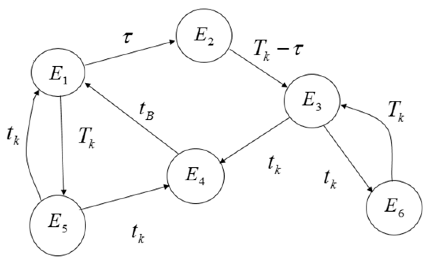
A continuously operating CTS with periodic verification of the technical condition is ready for use at that time $\tau$ if it is operational at that moment and is not under verification or repair. The results of the control are used to make a decision on the possibility of further application of the CTS. If the CTS is recognized as workable, according to the results of the verification, then it is included in the work. If the CTS is found to have failed, then its repair is carried out, as a result of which a complete restoration of its operability occurs. The transition graph is shown in Figure 1.

Possible conditions of the CTS: $E_1$ is workable, $E_2$ is unworkable (failure), $E_3$ is verification of the failed CTS, $E_4$ is recovery, $E_5$ is verification of a workable CTS, and $E_6$ is undetected failure.

The transition probability matrix has the following form:

$$P^{*}=\left(\begin{array}{cccccc}0& F(T_K)& 0& 0& 1-F(T_K)& 0\\ 0& 0& 1& 0& 0& 0\\ 0& 0& 0& 1-\beta & 0& \beta \\ 1& 0& 0& 0& 0& 0\\ 1-\alpha & 0& 0& \alpha & 0& 0\\ 0& 0& 1& 0& 0& 0\end{array}\right),$$

where $F(\tau )$ is the integral function of the distribution of the failure time, $F(T_K)$ is the probability of failure during the time between two verifications, $T_K$ is the time interval between verifications (TIBV) of the technical condition, $\alpha$ is the conditional probability of a false failure, and $\beta$ is the conditional probability of an undetected failure.

We assume that the duration of the control (verification of the technical condition) and the duration of the restoration (repair) are deterministic values equal to $t_K$ and $t_B$, respectively.

The system of equations for finding ${\pi }_i$, $i=1,2,\dots ,6$ has the form:

$$\begin{gathered} {\pi }_1={\pi }_4+(1-\alpha ){\pi }_5,{\pi }_2=F(T_K){\pi }_1,{\pi }_3={\pi }_2+{\pi }_6,{\pi }_4=(1-\beta ){\pi }_3+\alpha {\pi }_5, \\ {\pi }_5=\left[1-F(T_K)\right]{\pi }_1,{\pi }_6=\beta {\pi }_3,{\pi }_1+{\pi }_2+{\pi }_3+{\pi }_4+{\pi }_5+{\pi }_6=1. \end{gathered}$$

The solution of the system has the form:

$$\left\{\begin{array}{l}{\pi }_1=\frac{1}{A}(1-\beta )\hfill \\ {\pi }_2=\frac{1}{A}F(T_K)(1-\beta )\hfill \\ {\pi }_3=\frac{1}{A}F(T_K)\hfill \\ {\pi }_4=\frac{1}{A}\left\{F(T_K)+\alpha (1-F(T_K)\right\}(1-\beta )\hfill \\ {\pi }_5=\frac{1}{A}\left[1-F(T_K)\right](1-\beta )\hfill \\ {\pi }_6=\frac{1}{A}{\beta }^{}F(T_K)\hfill \end{array}\right.,$$

(2)

where $A=2\left[1-\beta +F(T_K)\right]+\alpha \left[1-F(T_K)\right](1-\beta )$.

The values $v_i$, $i=1,2,\dots ,6$ are equal to:

$$\left\{\begin{array}{l}{v}_1={\displaystyle \underset{0}{\overset{T_K}{\int }}\tau dF(\tau )+T_K\left[1-F(T_K)\right]}\hfill \\ v_2=T_{K}F(T_K)-{\displaystyle \underset{0}{\overset{T_K}{\int }}\tau dF(\tau )}\hfill \\ v_3=t_K\hfill \\ v_4=t_B\hfill \\ v_5=t_K\hfill \\ v_6=T_K\hfill \end{array}\right..$$

(3)

Assuming that $w_1=v_1$, $w_2=0$, $w_3=0$, $w_4=0$, $w_5=0$, $w_6=0$, and substituting (2) and (3) into (1), we obtain the formula for calculating the CTS readiness coefficient:

$$K_A=\frac{I+T_{K}B}{BI+T_K\left\{B+{\left[F(T_K)\right]}^2+\frac{\beta F(T_K)}{1-\beta }\right\}+t_k\left[B+\frac{F(T_K)}{1-\beta }\right]+t_B\left[F(T_K)+\alpha B\right]},$$

(4)

where $B=1-F(T_K)$, $I={\displaystyle \underset{0}{\overset{T_K}{\int }}\tau \cdot dF(\tau )}$.

Next, we will conduct a study of the readiness coefficient for various laws on the distribution of the failure time. The failure time of the CTS is considered as a random variable. Analysis of statistical data has shown that the most suitable laws for describing the failure time are the exponential law, Rayleigh’s law, the Weibull distribution and the truncated normal distribution, with the appropriate choice of parameters for these distributions. The statistical function of the distribution of the failures is located inside the “curved band” covering the theoretical distribution functions.

In the case of the exponential distribution law, the expression for the readiness coefficient (4) takes the form:

$$K_{\Gamma }=\frac{1-e^{-\lambda T_K}}{\left(\frac{\lambda T_K}{1-\beta }+e^{-\lambda T_K}\right)\cdot \left(1-e^{-\lambda T_K}\right)+\lambda t_k\left(\frac{(1-e^{-T_K}){\beta }_p}{1-\beta }+1\right)+\lambda t_B\left(1-e^{-\lambda T_K}(1-{\alpha }_p)\right)}.$$

For Rayleigh’s law, the integral $I$ can be calculated numerically or using the standard Laplace function, for Weibull’s law it can be calculated numerically or using the gamma function; and for the truncated normal distribution it can be calculated numerically or using the standard Laplace function.

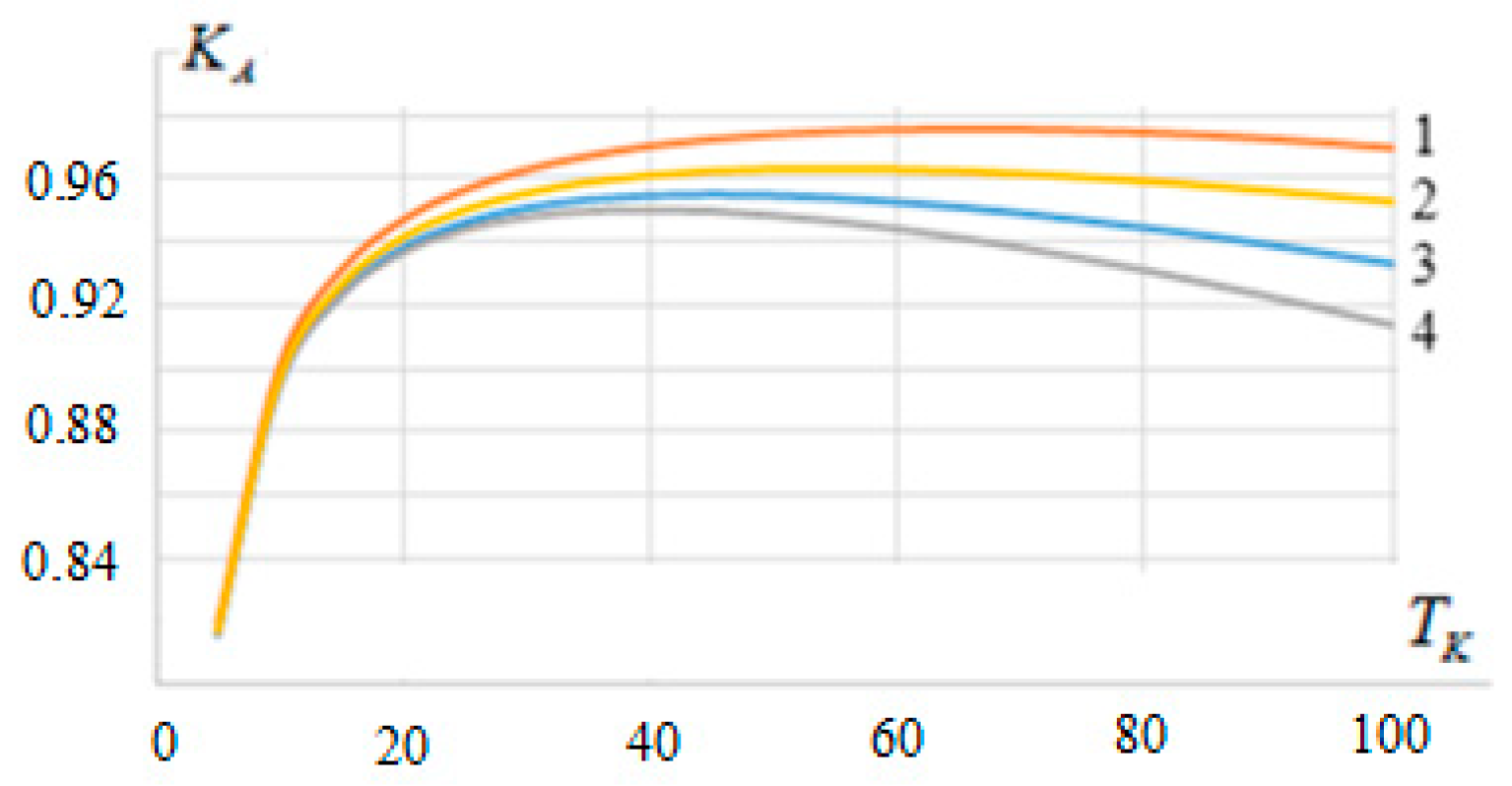
The calculations were carried out using the following values from the initial data: $t_K=1$, $t_B=1$, $\alpha =0.1$, $\beta =0.1$, and $\lambda =0.0025$ for the different values of $T_K$. Figure 2 shows the dependences of the readiness coefficients $K_A$ on the periodicity of the verification $T_K$, for the distribution laws described above. The maximum values of $K_A$ for the Rayleigh, normal, exponential and Weibull laws are equal to: 0.976, 0.963, 0.955, and 0.950, respectively, and reach values equal to 65, 55, 50, and 40. Note that the maximum value of the coefficient for each distribution law is reached at a single point. It can be seen that $\max K_A$ is “practically insensitive” to $T_K$. So, in a fairly wide range of changes to $T_K$, the readiness coefficient takes values close to the maximum. In particular, when changes to $T_K$ take place in the range $25\le T_K\le 60$, the variation of $K_A$ is no more than 2–3%.

The low sensitivity of the maximum value of the readiness coefficient to the periodicity of the technical condition monitoring makes it possible to develop strategies that are “non-strict” and easy to implement in practice, for carrying out checks on the technical condition of the CTS with metrological support.

4.1.2. Development of the Classical Model: The Model of False and Undetected Failures

The probabilities of false and undetected failures [8] for the specific samples of the CTS depend on the corresponding probabilities of false and undetected failures of the individual components of the CTS (1), (2), on the configuration of the CTS using methods on the redundancy of the components, nodes and blocks of the CTS.

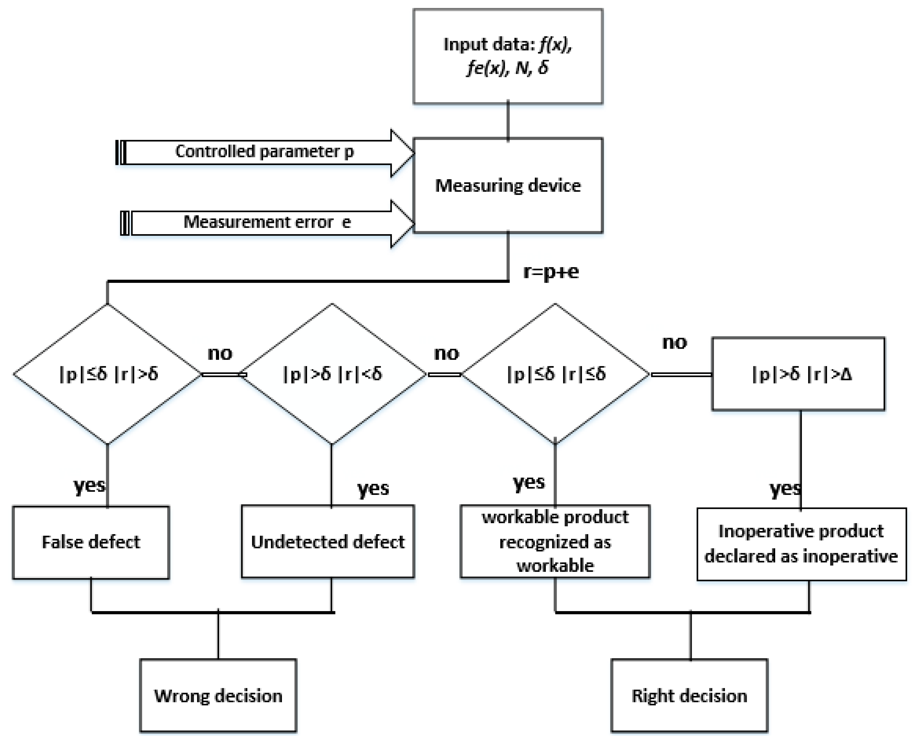
Let $p$ be the actual value of the measured (controlled) parameter and $\epsilon$ be the measurement error. The measurement result is presented in the form $r=p+\epsilon$. The general scheme of the diagnosis and decision-making based on the one-parameter method of tolerance control is shown in Figure 3.

Here $\delta$ is the tolerance for the controlled parameter, and $f(x)$ and $f_e(x)$ are the distribution density functions of the measured parameter and the measurement error, respectively. It can be seen that the probability of making the right decision can be increased (within certain limits) by reducing the total error of the erroneous decision.

The different physical nature and, consequently, the heterogeneous range of the changes in the measured values leads to the need to introduce dimensionless standardized operational parameters for the MI. As a normalizing element, we take the mean square deviation ${\mathsf{\sigma }}_x$ of the measured parameter $x$; $\mathsf{\delta }=\Delta /{\mathsf{\sigma }}_x$ is the relative operational tolerance, where Δ is the technical tolerance; $z={\sigma }_{\epsilon }/{\mathsf{\sigma }}_x$ is the relative parametric measurement error, ${\mathsf{\sigma }}_{\mathsf{\epsilon }}$ is the mean square deviation of the MI error.

The model is based on formulas for the conditional probabilities of false and undetected failures, respectively [8]:

$$\mathsf{\alpha }(\mathsf{\delta },z)=\left\{{\displaystyle \underset{-\mathsf{\delta }}{\overset{\mathsf{\delta }}{\int }}{f}_{cu}(y)\left({\displaystyle \underset{-\infty }{\overset{\frac{-\mathsf{\delta }-y}{z}}{\int }}{f}_o(\mathsf{\tau })d\mathsf{\tau }+{\displaystyle \underset{\frac{\mathsf{\delta }-y}{z}}{\overset{\infty }{\int }}{f}_o(\mathsf{\tau })d\mathsf{\tau }}}\right)dy}\right\}/\left\{{\displaystyle \underset{-\mathsf{\delta }}{\overset{\mathsf{\delta }}{\int }}{f}_{cu}(y)dy}\right\},$$

(5)

$$\beta (\mathsf{\delta },z)=\left\{{\displaystyle \underset{-\infty }{\overset{-\mathsf{\delta }}{\int }}{f}_{cu}(y)\left({\displaystyle \underset{\frac{-\mathsf{\delta }-y}{z}}{\overset{\frac{\mathsf{\delta }-y}{z}}{\int }}{f}_0(\mathsf{\tau })d\mathsf{\tau }}\right)dy+{\displaystyle \underset{\mathsf{\delta }}{\overset{\infty }{\int }}{f}_{cu}(y)\left({\displaystyle \underset{\frac{-\mathsf{\delta }-y}{z}}{\overset{\frac{\mathsf{\delta }-y}{z}}{\int }}{f}_0(\mathsf{\tau })d\mathsf{\tau }}\right)dy}}\right\}/\left\{{\displaystyle \underset{-\infty }{\overset{-\mathsf{\delta }}{\int }}{f}_{cu}(y)dy+{\displaystyle \underset{\mathsf{\delta }}{\overset{\infty }{\int }}{f}_{cu}(y)dy}}\right\},$$

(6)

where $f_0(\tau )$ and $f_{cu}(y)$ are the functions of the distribution densities of the measured value and the MI error, respectively.

For normally distributed measured values and MI errors, Formulas (5) and (6) take the form:

$$\alpha (\mathsf{\delta },z)=\frac{1}{2\pi }\left\{{\displaystyle \underset{-\mathsf{\delta }}{\overset{\mathsf{\delta }}{\int }}\exp \left(-\frac{y^2}{2}\right)\left({\displaystyle \underset{-\infty }{\overset{\frac{-\mathsf{\delta }-y}{z}}{\int }}\exp \left(-\frac{{\mathsf{\tau }}^2}{2}\right)d\tau +{\displaystyle \underset{\frac{\mathsf{\delta }-y}{z}}{\overset{\infty }{\int }}\exp \left(-\frac{{\mathsf{\tau }}^2}{2}\right)d\mathsf{\tau }}}\right)dy}\right\}/P1,$$

(7)

$$\beta (\mathsf{\delta },z)=\frac{1}{2\pi }\left\{{\displaystyle \underset{-\infty }{\overset{-\mathsf{\delta }}{\int }}\exp \left(-\frac{y^2}{2}\right)\left({\displaystyle \underset{\frac{-\mathsf{\delta }-y}{z}}{\overset{\frac{\mathsf{\delta }-y}{z}}{\int }}\exp \left(-\frac{{\mathsf{\tau }}^2}{2}\right)d\mathsf{\tau }}\right)dy+{\displaystyle \underset{\mathsf{\delta }}{\overset{\infty }{\int }}\exp \left(-\frac{y^2}{2}\right)\left({\displaystyle \underset{\frac{-\mathsf{\delta }-y}{z}}{\overset{\frac{\mathsf{\delta }-y}{z}}{\int }}\exp \left(-\frac{{\mathsf{\tau }}^2}{2}\right)d\mathsf{\tau }}\right)dy}}\right\}/P2,$$

(8)

$$P1=\frac{1}{\sqrt{2\pi }}{\displaystyle \underset{-\mathsf{\delta }}{\overset{\mathsf{\delta }}{\int }}\exp \left(-\frac{y^2}{2}\right)dy},P2=\frac{1}{\sqrt{2\pi }}\left\{{\displaystyle \underset{-\infty }{\overset{-\mathsf{\delta }}{\int }}\exp \left(-\frac{y^2}{2}\right)dy+{\displaystyle \underset{\mathsf{\delta }}{\overset{\infty }{\int }}\exp \left(-\frac{y^2}{2}\right)dy}}\right\}$$

For other distribution laws on the measured value and measurement error, the model (5), (6) were investigated in [8].

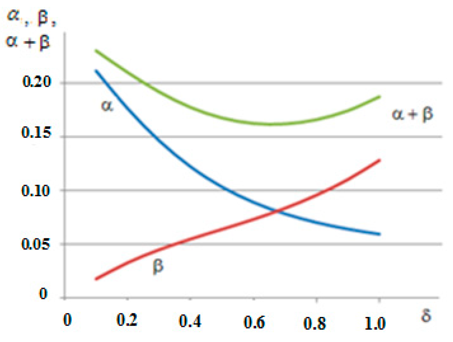
The dependences of the probabilities $\alpha (\delta ,z)$ and $\mathsf{\beta }(\mathsf{\delta },z)$, as well as the probability $\mathsf{\alpha }(\mathsf{\delta },z)+\mathsf{\beta }(\mathsf{\delta },z)$ of an erroneous decision $\delta$ on the tolerance value at $z=0.5$ are shown in Figure 4.

Note also that the error solution function reaches its minimum at some internal point $\delta \in (0{;}^{}1)$, as is the case with the normal distribution of the measured value and the measurement error.

The two-dimensional dependences of the probabilities of false and undetected failures on the magnitude of the dimensionless measurement error $z$ and the dimensionless tolerance for the controlled parameter $\mathsf{\delta }$ are shown in Figure 5a,b.

4.1.3. Development of the Classical Model: Models of Failures and Degradation of the Complex Technical System

All failure models that allow for the taking into account of the degradation processes occurring in the CTS can be conditionally divided into probabilistic, empirical, and probabilistic physical models, that includes among other things, the Markov models of degradation and failures.

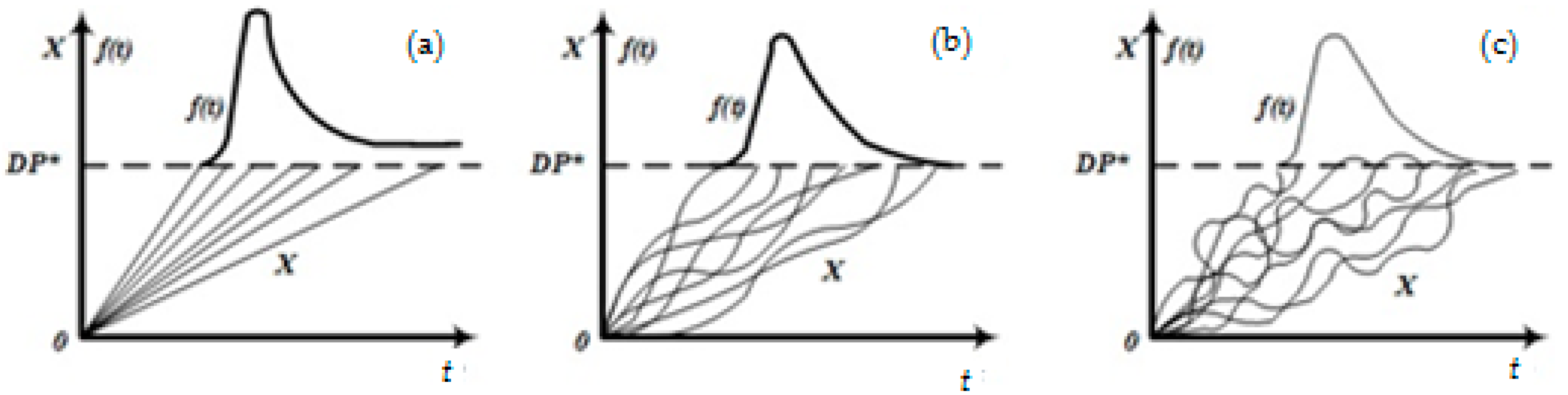
In the fan model [9,10,11], also called a distribution and belonging to the category of probabilistic models, the defining parameter (DP) is represented as a linear function of time, shown in Figure 6a.

Here, $t$ is the operating time for the failure; $X$ is random variable of the DP; DP* is the normalized value of the DP at which the failure occurs; and $f$ is the function of density of the distribution of the operating time for the failure.

The distribution function of the operating time up to a given level DP* is given by the distribution function [9,10,11]:

$$F(t)=\Phi \left(\frac{t-\mu }{vt}\right),$$

(9)

where $\Phi$ is the normalized normal distribution function; $\mu =1/a$ is the parameter of the scale of degradation, $a$ is the mathematical expectation of the rate of change of the DP (the average rate of the degradation process), normalized to the limit value; and $\nu$ is the shape parameter (coefficient of the variation of the degradation process).

The empirical model of the “drift of metrological characteristics” [6,7] is based on the assumption on a linear law of change of the MI zero mark and an exponential law of increasing measurement error:

$$m_0(t)=m_{00}+v_{m}t,\sigma (t)={\sigma }_0+\frac{v_z}{a_z}\left(\exp (a_{z}t)-1\right),$$

(10)

where ${\sigma }_0$ is the value of the initial error, $v_z$ is the average initial velocity of the error increase, $a_z$ is the parameter characterizing the acceleration of the error increase, $m_{00}$ is the initial value of the zero drift (usually assumed to be zero), and $v_m$ is the average velocity of the zero drift.

Let us now consider the Markov models of degradation and failures, widely used in applied problems. In these models, it is assumed that the degradation process can be approximated by a continuous Markov process of the diffusion type [9,10,11] and is described by a stochastic differential equation of the Ito type:

$$dx(t)=A(t)dt+B(t)d\eta (t),$$

(11)

where $x(t)$ is the value of the DP; $A(t)$ and $B(t)$ are deterministic functions characterizing the change in the mean value and variance of the DP (drift coefficient and diffusion coefficient); and $\eta (t)$ is a random variable of the Gaussian type.

The problem of determining the distribution of time before the first failure of the MI, in this case, is reduced to solving the problem of the first achievement of the upper limit of the DP* (see Figure 6b,c). This problem can be solved if the conditional probability density $\omega (t,x)$ of the process transition from one state to another is known.

For a Markov diffusion-type processes, a partial differential equation (the Fokker–Planck–Kolmogorov equation) follows from (11):

$$\frac{\partial \omega (t,x)}{\partial t}+A(t)\frac{\partial \omega (t,x)}{\partial x}-\frac{{\left(B(t)\right)}^2}{2}\frac{{\partial }^2\omega (t,x)}{\partial x^2}=0,$$

(12)

where $A(t)$ and $B(t)$ are the coefficients of the equation depending on the operating conditions of the MI, and the physical and chemical processes occurring in the materials from which the MI is made. To solve (12), it is necessary to set boundary conditions that depend on the type of implementation of a random process, in particular, on their monotonic nature (Figure 6b) or non-monotonic nature (Figure 6c). You also need to set the initial conditions: $t=t_0$, $x=x_0$.

After finding the function $\omega (t_0,x_0;t,x)$, satisfying the given initial conditions, the density function $f(t)$ of the distribution of the time to reach the boundary DP* (the density function of the distribution of the time to failure) can be calculated by the formula [11]:

$$f(t)=-{\displaystyle \underset{-\infty }{\overset{t}{\int }}\frac{\partial \omega (t_0,x_0;t,x)}{\partial t}dx}$$

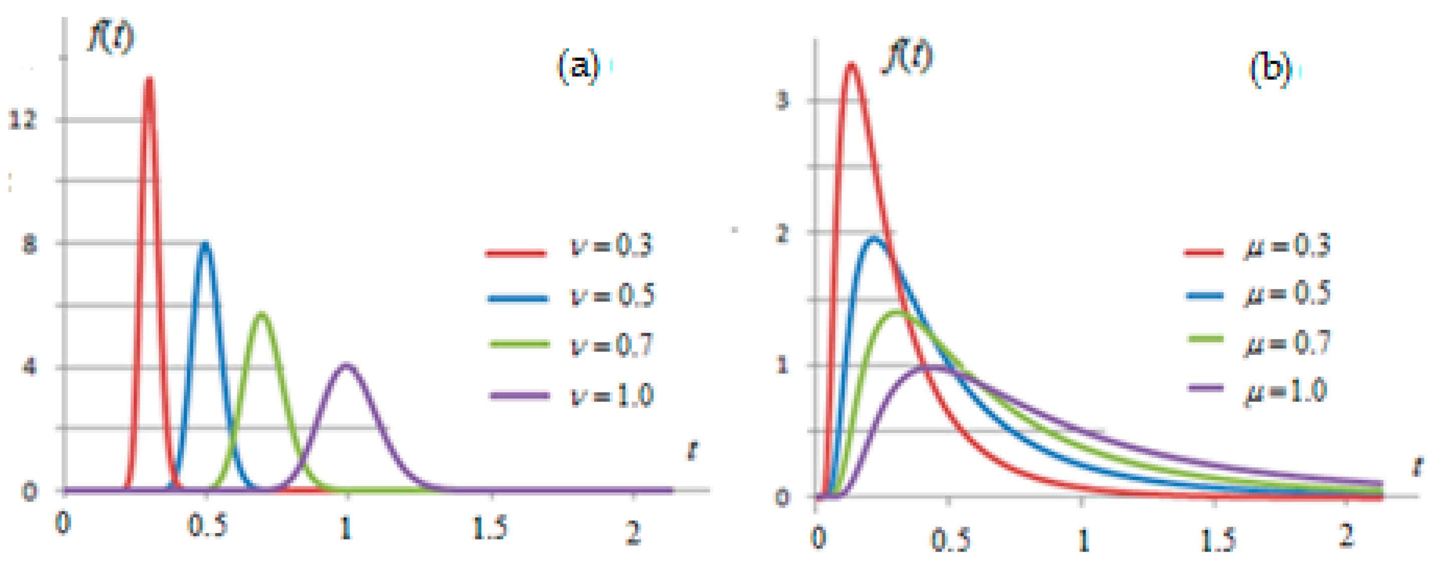
In case of one DP, Equation (12) can be integrated analytically. The distribution function for the diffusion monotone distribution (DM distribution) has the form [11]:

$$F(t)=DM(t;\mu ,\nu )=\Phi \left(\frac{t-\mu }{v\sqrt{\mu t}}\right),$$

(13)

Here, $\mu =1/a$.

The distribution density function $f(t)$ for (13) at $\mu =0.1$ is shown in Figure 7a.

The distribution function for the diffusion non-monotonic distribution (DN distribution) has the form [11]:

$$F(t)=DN(t;\mu ,\nu )=\Phi \left(\frac{t-\mu }{v\sqrt{\mu t}}\right)+\exp \left(\frac{2}{{\nu }^2}\right)\Phi \left(-\frac{t-\mu }{v\sqrt{\mu t}}\right).$$

(14)

The corresponding distribution density functions $f(t)$ for (14) at $\nu =0.8$ are shown in Figure 7b.

The failure rates for DM distribution and DN distribution have the form:

$${\lambda }_{DM}(t)=\frac{(t+\mu )\exp \left(-\frac{{(t-\mu )}^2}{2{\nu }^2\mu t}\right)}{2\nu t\sqrt{2\pi \mu t}\cdot \Phi \left(\frac{\mu -t}{v\sqrt{\mu t}}\right)},{\lambda }_{DN}(t)=\frac{{\left(\nu t\sqrt{2\pi t}\right)}^{-1}\sqrt{\mu }\cdot \exp \left(-\frac{{(t-\mu )}^2}{2{\nu }^2\mu t}\right)}{\Phi \left(\frac{\mu -t}{v\sqrt{\mu t}}\right)-\exp \left(\frac{2}{{\nu }^2}\right)\cdot \Phi \left(-\frac{\mu -t}{v\sqrt{\mu t}}\right)}$$

Thus, distribution density functions $f(t)$, distribution functions $F(t)$, and failure rate functions $\lambda (t)$, are calculated using finite analytical formulas using the standard Laplace function $\Phi (t)$.

In case of several DP distribution densities $f(t)$, distribution functions $F(t)$, and failure rates $\lambda (t)$, can only be calculated numerically.

The process of degradation of the mechanical components of the CTS, due to the irreversibility of the destruction processes (mechanical wear, fatigue straining, etc.), is considered to be a process with monotonous realizations of a random variable. DM distribution is used for CTS nodes containing electromechanical elements (relay and connector contacts, sliding electrical contacts, gears, etc.) [11].

The process of degradation of the CTS, which include integrated circuits and complex electronic devices, also has non-monotonic implementations of a random variable. Therefore, the degradation of such CTS is described by the DN distribution [11].

We will analyze the models of failures and degradation of the CTS. Degradation and failures models differ significantly from a physical point of view. In particular, the fan process assumes that its characteristics are completely determined by the initial state (the quality of the manufacturing samples of the components of the CTS), and do not depend on the mechanical, physical and chemical degradation processes occurring in the circuits and mechanisms of the components of the CTS, under the influence of external conditions and time.

The drift model of metrological characteristics [10], clearly demonstrates the departure of the zero mark of the MI and CTS with the increase in measurement error over time. The model assumes preliminary processing of statistical data in order to determine estimates of the drift parameters.

The Markov models (12), (13) are based on the use of probabilistic characteristics, the operating conditions of the CTS, as well as on the use of the physical and chemical properties of the materials. The advantage of Markov models [12,13] is that they have accurate analytical expressions for all statistical characteristics, including statistical moments. In addition, there are no analytical expressions for the statistical moments of the fan $\alpha$ distribution law. These moments are determined by approximate dependencies, which complicates the use of a fan distribution in practice.

The density distribution function of the DM distribution occupies an intermediate position between the, widely used in practice, normal distribution (which is symmetrical) and the more elongated distribution.

The density curves of the DN distribution have a more significant insensitivity threshold, a more positive kurtosis and are more asymmetric than the DM distribution.

The intensities of the diffusion distributions have finite limits:

$$\underset{t\to \infty }{\lim }{\lambda }_{DM}(t)=\underset{t\to \infty }{\lim }{\lambda }_{DN}(t)=\frac{1}{2\mu {\nu }^2}.$$

Here, are some important properties of diffusion distributions for practical application:

1. Where a random variable $T$ is described by a DM distribution of the form $DM(t;\mu ,\nu )$, then the random variable $x=cT$ ($c=const$) is also described by a DM distribution of the form $DM(t;c\mu ,\nu )$.

2. Where a random variable $T$ is described by a DM distribution of the form $DM(t;\mu ,\nu )$, then the random variable $\theta =\frac{1}{T}$ is also described by a DM distribution of the form $DM\left(t;\frac{1}{\mu },\nu \right)$.

3. Where a random variable $T$ is described by a DN distribution of the form $DN(t;\mu ,\nu )$, then the random variable $x=cT$ ($c=const$) is also described by a DN distribution of the form $DN(t;c\mu ,\nu )$.

4. The sum of $n$ random variables obeying the distribution of the form $DN(t;\mu ,{\nu }_i)$ is described by the DN distribution of the form $DN\left(t;n\mu ,1/\sqrt{{\displaystyle \sum _{i=1}^n{\nu }_i^{-2}}}\right)$.

5. The sum of n random variables obeying a distribution of the form $DN(t;{\mu }_i,\nu )$ is described by a DN distribution of the form $DN\left(t;{\displaystyle \sum _{i=1}^n{\mu }_i^{}},\nu /\sqrt{n}\right)$.

6. The sum of $n$ random variables obeying the DN distribution of the form $DN(t;\mu ,\nu )$ is described by the DN distribution of the form $DN\left(t;n\mu ,\frac{\nu }{\sqrt{n}}\right)$.

The proof of properties 1–6 can be carried out by replacing the variables and definitions of functions (13)–(14).

Some additional properties of diffusion distributions are described in [11].

Analysis of the graphs on the distribution functions shows that distributions (9), (12), (13) have different zones of high reliability. This means that the estimation of small-level quantiles, i.e., the assignment of a gamma-percent resource, significantly depends on the selected type of failure model of the CTS.

Diffusion models can be parameterized quite simply in the presence of statistical information. For example, when parameterizing based on statistical data on the moments of failure $\left\{t_i,(i=1,2,\dots ,N)\right\}$, the estimates of the parameters $\stackrel{⌣}{\mu }$ and $\stackrel{⌣}{\nu }$ calculated using the maximum likelihood method for the DM distribution have the form:

$$\stackrel{⌣}{\mu }=\frac{1}{N}{\displaystyle \sum _{i=1}^N{t}_i},\stackrel{⌣}{\nu }=\sqrt{\stackrel{⌣}{\mu }}\cdot \sqrt{\frac{1}{N}{\displaystyle \sum _{i=1}^N\frac{1}{t_i}}-N{\left({\displaystyle \sum _{i=1}^N{t}_i}\right)}^{-1}},$$

and for DN distributions have the form:

$$\stackrel{⌣}{\mu }=N{\left({\displaystyle \sum _{i=1}^N\frac{1}{t_i}}\right)}^{-1}+\frac{N}{2}{\left({\displaystyle \sum _{i=1}^N{(\stackrel{⌣}{\mu }+t_i)}^{-1}}\right)}^{-1}-\frac{N^2}{4}{\left({\displaystyle \sum _{i=1}^N{(\stackrel{⌣}{\mu }+t_i)}^{-1}}\right)}^{-2}-N{\left({\displaystyle \sum _{i=1}^N\frac{1}{t_i}}\right)}^{-1}\sqrt{\frac{1}{N}{\displaystyle \sum _{i=1}^N{t}_i}-N{\left({\displaystyle \sum _{i=1}^N\frac{1}{t_i}}\right)}^{-1}},$$

$$\stackrel{⌣}{\nu }=\sqrt{\frac{1}{\stackrel{⌣}{\mu }N}{\displaystyle \sum _{i=1}^N{t}_i}+\frac{\stackrel{⌣}{\mu }}{N}{\displaystyle \sum _{i=1}^N\frac{1}{t_i}-2}}$$

Thus, diffusion models are more preferable (adequate), since, unlike the fan distribution and the drift model of metrological characteristics, they can be used to control the degradation and reliability of the CTS, based on the taking into account of the physical patterns implemented through time-dependent variable coefficients $A(t)$ and $B(t)$ in Equation (12). The task of developing models of physical processes for the purpose of constructing coefficients $A(t)$ and $B(t)$ is an independent scientific task and is not considered in this article.

4.2. The Model of Operation of a Complex Technical System Fleet with a Fully Recoverable Resource

The attribution of a set of CTS to one or another degradation group is carried out on the basis of structural and functional analysis of the metrological reliability indicators [2,6,7], which includes the types of failures, the consequences of the failures, as well as determination and analysis of the rational composition of the controlled parameters and an assessment of the required recovery time of the CTS. In this paper, the controlled states of the CTS will be evaluated using the probabilities of a false failure $\alpha$, an undetected failure $\beta$ and the time $t_B$ required for recovery after the failure is detected (the recovery time depends on the “severity” of the malfunction detected during monitoring). At low values of these estimated indicators, we will refer the CTS to the first group of degradation. As the degradation increases (as these indicators increase), we will refer the CTS to the second, third and fourth groups of degradation, respectively. Without going into the details of assigning parameters of criteria for attribution to a particular degradation group, we note that the number of degradation levels is determined by a set of types and types of CTS under consideration, their characteristic features, as well as the specific task being solved.

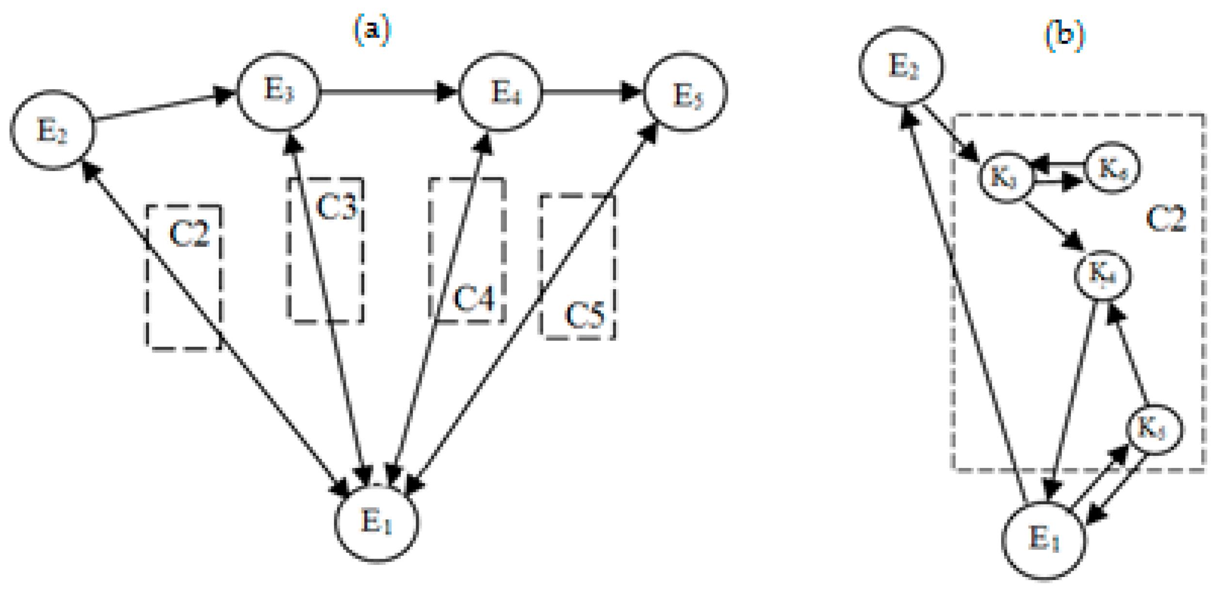
Figure 8a shows a graph with one fully workable state $E_1$ and four states corresponding to different levels of degradation (malfunction): $E_2$, $E_3$, $E_4$ and $E_5$ [6]. Let us distinguish the three parts in the classical model [2]: the initial operational state $E_1$, the failure state $E_2$ and the subgraph corresponding to the control function (highlighted in Figure 8b by rectangle C2). Then, the classical model can be represented as a “serial connection” $E_1$, C2 and $E_2$ [14,15]. The states of the subgraph: $K_3$ is verification of a failed MI, $K_4$ is the restoration of the CTS, $K_5$ is verification of a working MI and $K_6$ is the state of an undetected failure of the CTS. The probabilistic characteristics of the state transition are the same as in the classical model [2].

Note that if the control subgraph is completely removed from the graph in Figure 8b and the probabilistic characteristics are set on the edges of the remaining graph, then a simple model will be obtained that describes the operation of a small gun [6].

Figure 8a uses the notation: E₁ is a fully functional state and four states corresponding to different levels of degradation of the CTS; E₂ is the first group of degradation (functional state with minor deviations of the normalized metrological characteristics); E₃ is the second group of degradation (a state with some deviations of the metrological characteristics, from which it is possible to return to a fully functional state with small resource costs); E₄ is the third group degradation (a state from which it is possible to return to a fully functional state with costs associated with sufficiently resource-intensive maintenance); and E₅ is the fourth “heavier” group of degradation. As the degradation group number increases, returning to the state E₁ becomes more and more resource intensive.

Let us “attach” four metrological control systems, C2, C3, C4 and C5, between the fully functional state $E_1$ and the other four states, similar to the one shown in Figure 8a (“fan connection”). We will use the corresponding upper indices for the probabilistic and deterministic parameters of the model of each subsystem, describing samples of the CTS with different levels of degradation.

Then, the system of equations describing the semi-Markov stationary model will take the form [6]:

$$\left\{\begin{array}{l}{\pi }_1^{(1)}={\pi }_4^{(1)}+(1-{\alpha }_1){\pi }_5^{(1)}+{\pi }_4^{(2)}+(1-{\alpha }_2){\pi }_5^{(2)}+{\pi }_4^{(3)}+(1-{\alpha }_3){\pi }_5^{(3)}+{\pi }_4^{(4)}+(1-{\alpha }_4){\pi }_5^{(4)}\hfill \\ {\pi }_2^{(1)}={\gamma }_1{\pi }_1^{}\hfill \\ {\pi }_3^{(1)}=(1-{\delta }_1){\pi }_2^{(1)}+{\pi }_6^{(1)}\hfill \\ {\pi }_4^{(1)}=(1-{\beta }_1){\pi }_3^{(1)}+{\alpha }_1{\pi }_5^{(1)}\hfill \\ {\pi }_5^{(1)}=\left[1-{\gamma }_1\right]{\pi }_1\hfill \\ {\pi }_6^{(1)}={\beta }_1{\pi }_3^{(1)}\hfill \end{array},\right.$$

$$\left\{\begin{array}{l}{\pi }_2^{(2)}={\gamma }_2{\pi }_1^{}+{\delta }_1{\pi }_2^{(1)}\hfill \\ {\pi }_3^{(2)}=(1-{\delta }_2){\pi }_2^{(2)}+{\pi }_6^{(2)}\hfill \\ {\pi }_4^{(2)}=(1-{\beta }_2){\pi }_3^{(2)}+{\alpha }_2{\pi }_5^{(2)}\hfill \\ {\pi }_5^{(2)}=\left[1-{\gamma }_2\right]{\pi }_1\hfill \\ {\pi }_6^{(2)}={\beta }_2{\pi }_3^{(2)}\hfill \end{array}\right.,\left\{\begin{array}{l}{\pi }_2^{(3)}={\gamma }_3{\pi }_1^{}+{\delta }_2{\pi }_2^{(2)}\hfill \\ {\pi }_3^{(3)}=(1-{\delta }_3){\pi }_2^{(3)}+{\pi }_6^{(3)}\hfill \\ {\pi }_4^{(3)}=(1-{\beta }_3){\pi }_3^{(3)}+{\alpha }_3{\pi }_5^{(3)}\hfill \\ {\pi }_5^{(3)}=\left[1-{\gamma }_3\right]{\pi }_1\hfill \\ {\pi }_6^{(3)}={\beta }_2{\pi }_3^{(3)}\hfill \end{array}\right.,\left\{\begin{array}{l}{\pi }_2^{(4)}={\gamma }_4{\pi }_1^{}+{\delta }_3{\pi }_2^{(3)}\hfill \\ {\pi }_3^{(4)}={\pi }_2^{(4)}+{\pi }_6^{(4)}\hfill \\ {\pi }_4^{(4)}=(1-{\beta }_4){\pi }_3^{(4)}+{\alpha }_4{\pi }_5^{(4)}\hfill \\ {\pi }_5^{(4)}=\left[1-{\gamma }_4\right]{\pi }_1\hfill \\ {\pi }_6^{(4)}={\beta }_4{\pi }_3^{(4)}\hfill \end{array}\right.$$

(15)

Here, ${\alpha }_i$, ($i=2,3,4,5$) is the conditional probability of a false failure, ${\beta }_i$ is the conditional probability of an undetected failure and ${\gamma }_i=F_i(T_K)$${\delta }_j,(j=1,2,3)$ are the probability of a transition from a state of degradation to the next, more severe, state number $j+1$.

Model (15) is a system of 21 equations. The rank of the system is 20. Exclude one of the equations (for example, the last equation of the system (15)) and add a normalization condition, as follows:

$${\pi }_1+{\displaystyle \sum _{i=1}^4{\displaystyle \sum _{j=2}^6{\pi }_j^{(i)}}}=1$$

(16)

Then, the resulting system of linear inhomogeneous Equations (15) and (16) will have a unique solution that can be obtained using standard algorithms and methods for solving the corresponding systems [5,6].

Initial data: the total number of states is 21 and the number of degradation levels is four. As the CTS degrades, the duration of the verification and recovery time increase, and reliability decreases.

As generalized parameters characterizing the distribution of the control volumes by the degradation groups, the duration TIBV $T_K^{(i)}$ for each of the four degradation groups was selected. As a result of the calculations, the dependence of the readiness coefficient on the TIBV was constructed:

$$K_A=K_A(T_K^{(1)},T_K^{(2)},T_K^{(3)},T_K^{(4)}),$$

(17)

and the analysis of the influence of the TIBV of the different degradation groups (i = 1, 2, 3, 4) on the readiness coefficient was carried out. When constructing the dependence (17), the probabilities of false and undetected failures were set as average values for each of the degradation groups, namely: ${\alpha }_4>{\alpha }_3>{\alpha }_2>{\alpha }_1$, ${\beta }_4>{\beta }_3>{\beta }_2>{\beta }_1$.

The calculations have shown that if three arguments out of four are fixed in function (17), for example $T_K^{(2)}=c^{(2)*}$, $T_K^{(3)}=c^{(3)*}$, $T_K^{(4)}=c^{(4)*}$, $c^{(i)*}=const$ then the dependence of function (17) on the remaining variable $T_K^{(1)}$ will have the form shown in Figure 9. If two arguments out of four are fixed in function (17), for example $T_K^{(1)}=c^{(1)*}$ and $T_K^{(2)}=c^{(2)*}$ then the readiness coefficient $K_A$, as functions of two variables, will be convex upwards (Figure 9). The maximum of the readiness coefficient $K_A$ is reached at a single internal point. Here and further, an asterisk in the upper index means that the corresponding value is set and fixed.

The calculations have shown that the maximum value of the readiness coefficient is achieved if the TIBV for the fourth degradation group is about 1.3 times less than for the third group.

The developed model allows us to calculate the optimal duration of the TIBV for the CTS of different degradation groups. If it is impossible to provide optimal TIBV values for some degradation groups in practice, then in (17) “possible” TIBV values should be set for these groups and local optimum TIBV durations for the remaining degradation groups should be calculated.

Note that the model of interaction of the CTS with the MI with a simplified form of technical condition control can be represented as a graph (Figure 8a), if you remove the control subgraphs C2–C5 and set the probabilistic characteristics of the state transitions on the edges of the remaining graph. Such a model, supplemented with a formula for calculating the average total resource costs $SUM=S_{12}{p}_{12}+S_{23}{p}_{23}+S_{34}{p}_{34}+S_{45}{p}_{45}$ (where $S_{12},S_{23},S_{34},S_{45}$ are unit costs and $p_{12},p_{23},p_{34},p_{45}$ are probabilities of the state transitions), was used in [6] when calculating the technical and economic indicators of the metrological support system, when forming programs for the long-term development of the CTS fleet.

The models described in Section 4.1 and 4.2 do not allow modeling processes of CTS fleet renewal, and do not allow for the taking into account of the procurement of new CTS samples, or the modernization of existing CTS samples and the development of promising CTS samples. The model presented in Section 4.3 of the article allows modeling for all stages of the life cycle, including procurement, modernization and development of advanced CTS samples.

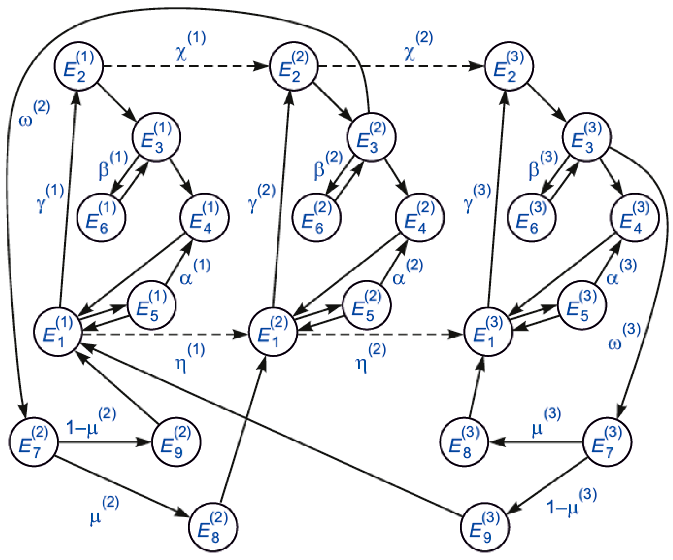
4.3. The Model of Operation of the Complex Technical System Fleet with a Partially Recoverable Resource

Next, we will distribute the CTS into three degradation groups [7]: the first is the start of operation of the CTS, the sample remains operational and the changes are insignificant; the second is where the operation and resource consumption of the CTS sample continue, the changes in characteristics are significant and the rate of change is average; and the third is a long-term operation, where the changes in characteristics are very significant and the rate of change is high. The number of degradation groups is determined by a set of types and the types of CTS under consideration, as well as the specific task being solved.

Figure 10 presents a graph of the operation model of the updated CTS fleet, with three degradation groups and two subgraphs modeling the process of updating the CTS fleet. The upper indices in parentheses indicate the number of the degradation group. Each degradation group will be modeled using the classical model [2], described in Section 4.1.1.

Each of the two subgraphs describing the upgrade process include three states: $E_7^{(l)},l=2,3$ are the in-depth diagnostics of the technical condition; $E_8^{(l)},l=2,3$ is the repair of the CTS; and $E_9^{(l)},l=2,3$ is the purchase (or development and production) of a new similar model of the CTS. The probabilistic parameters of the main state transitions are shown in Figure 10, in Greek letters. Certain shares of the CTS, from the second ω⁽²⁾ and third ω⁽³⁾ degradation groups, in case of failure of the CTS are sent for in-depth diagnostics of the technical condition, in order to determine the feasibility of updating (replacing with a new model of the CTS) or continuing operation after repair. To simplify, some probabilistic characteristics are not indicated in Figure 10, but they can be easily restored, taking into account that the sum of the probabilities of the transitions from each vertex of the graph are equal to one. If one edge comes out of the vertex, then the corresponding transition probability is one, and if two edges come out of the vertex, and the probability of one transition is written on the graph, then the probability of the second transition is equal to the difference of one and the known probability of the first transition.

The model of the management of the CTS fleet is presented structurally in the form of four systems of equations:

$$\left\{\begin{array}{l}{\mathsf{\pi }}_1^{(1)}={\mathsf{\pi }}_4^{(1)}+(1-{\mathsf{\alpha }}^{(1)}){\mathsf{\pi }}_5^{(1)}+{\mathsf{\pi }}_9^{(2)}+{\mathsf{\pi }}_9^{(3)}\hfill \\ {\mathsf{\pi }}_2^{(1)}={\mathsf{\gamma }}^{(1)}{\mathsf{\pi }}_1^{(1)}\hfill \\ {\mathsf{\pi }}_3^{(1)}=(1-{\mathsf{\chi }}^{(1)}){\mathsf{\pi }}_2^{(1)}+{\mathsf{\pi }}_6^{(1)}\hfill \\ {\mathsf{\pi }}_4^{(1)}=(1-{\mathsf{\beta }}^{(1)}){\mathsf{\pi }}_3^{(1)}+{\mathsf{\alpha }}^{(1)}{\mathsf{\pi }}_5^{(1)}\hfill \\ {\mathsf{\pi }}_5^{(1)}=\left[1-{\mathsf{\gamma }}^{(1)}-{\mathsf{\eta }}^{(1)}\right]{\mathsf{\pi }}_1^{(1)}\hfill \\ {\mathsf{\pi }}_6^{(1)}={\mathsf{\beta }}^{(1)}{\mathsf{\pi }}_3^{(1)}\hfill \end{array}\right.,\left\{\begin{array}{l}{\mathsf{\pi }}_1^{(2)}={\mathsf{\pi }}_4^{(2)}+(1-{\mathsf{\alpha }}^{(2)}){\pi }_5^{(2)}+{\mathsf{\eta }}^{(1)}{\mathsf{\pi }}_1^{(1)}+{\mathsf{\pi }}_8^{(2)}\hfill \\ {\mathsf{\pi }}_2^{(2)}={\mathsf{\gamma }}^{(2)}{\mathsf{\pi }}_1^{(2)}+{\mathsf{\chi }}^{(1)}{\mathsf{\pi }}_2^{(1)}\hfill \\ {\mathsf{\pi }}_3^{(2)}=(1-{\mathsf{\chi }}^{(2)}){\mathsf{\pi }}_2^{(2)}+{\mathsf{\pi }}_6^{(2)}\hfill \\ {\mathsf{\pi }}_4^{(2)}=(1-{\mathsf{\beta }}^{(2)}-{\mathsf{\omega }}^{(2)}){\mathsf{\pi }}_3^{(2)}+{\mathsf{\alpha }}^{(2)}{\mathsf{\pi }}_5^{(2)}\hfill \\ {\mathsf{\pi }}_5^{(2)}=\left[1-{\mathsf{\gamma }}^{(2)}-{\mathsf{\eta }}^{(2)}\right]{\mathsf{\pi }}_1^{(2)}\hfill \\ {\mathsf{\pi }}_6^{(2)}={\mathsf{\beta }}^{(2)}{\mathsf{\pi }}_3^{(2)}\hfill \end{array}\right.$$

$$\left\{\begin{array}{l}{\mathsf{\pi }}_1^{(3)}={\mathsf{\pi }}_4^{(3)}+(1-{\mathsf{\alpha }}^{(3)}){\mathsf{\pi }}_5^{(3)}+{\mathsf{\eta }}^{(2)}{\mathsf{\pi }}_1^{(2)}+{\mathsf{\pi }}_8^{(3)}\hfill \\ {\mathsf{\pi }}_2^{(3)}={\mathsf{\gamma }}^{(3)}{\mathsf{\pi }}_1^{(3)}+{\mathsf{\chi }}^{(2)}{\mathsf{\pi }}_2^{(2)}\hfill \\ {\mathsf{\pi }}_3^{(3)}={\mathsf{\pi }}_2^{(3)}+{\mathsf{\pi }}_6^{(3)}\hfill \\ {\mathsf{\pi }}_4^{(3)}=(1-{\mathsf{\beta }}^{(3)}-{\mathsf{\omega }}^{(3)}){\mathsf{\pi }}_3^{(3)}+{\mathsf{\alpha }}^{(3)}{\mathsf{\pi }}_5^{(3)}\hfill \\ {\mathsf{\pi }}_5^{(3)}=\left[1-{\mathsf{\gamma }}^{(3)}\right]{\mathsf{\pi }}_1^{(3)}\hfill \\ {\mathsf{\pi }}_6^{(3)}={\mathsf{\beta }}^{(3)}{\mathsf{\pi }}_3^{(3)}\hfill \end{array}\right.,\left\{\begin{array}{l}{\mathsf{\pi }}_7^{(2)}={\mathsf{\omega }}^{(2)}{\pi }_3^{(2)}\hfill \\ {\mathsf{\pi }}_8^{(2)}={\mu }^{(2)}{\mathsf{\pi }}_3^{(2)}\hfill \\ {\mathsf{\pi }}_7^{(3)}={\mathsf{\omega }}^{(3)}{\mathsf{\pi }}_3^{(3)}\hfill \\ {\mathsf{\pi }}_8^{(2)}={\mathsf{\mu }}^{(3)}{\mathsf{\pi }}_3^{(2)}\hfill \\ {\mathsf{\pi }}_9^{(2)}=\left[1-{\mathsf{\mu }}^{(2)}\right]{\mathsf{\pi }}_7^{(2)}\hfill \\ {\mathsf{\pi }}_9^{(3)}=\left[1-{\mathsf{\mu }}^{(3)}\right]{\mathsf{\pi }}_7^{(3)}\hfill \end{array}\right.$$

(18)

Here ${\mathsf{\pi }}_{\mathrm{i}}^{\left(\mathrm{j}\right)}$ are the stationary probabilities of finding the CTS in the corresponding states; ${\mathsf{\alpha }}^{(j)},j=1,2,3$, ${\mathsf{\beta }}^{(j)},j=1,2,3$ are the conditional probabilities of false and undetected failures, respectively; ${\mathsf{\gamma }}^{(j)}=F_j(T_K)$ is the probability of failure during the time interval $T_K$ between the verifications; $F_j(T)$ is exponential distribution function; and (${\chi }^{(j)},{\eta }^{(j)},j=1{,}^{}2$) are the probabilities of the transitions of the corresponding states from the $j$ degradation group to the next ($j+1$) group. The first three systems (18) describe the processes of the CTS operation for the three degradation groups, and the fourth system (18) describes the process of updating the CTS fleet.

Model (18) is a homogeneous system of 24 linear algebraic equations. The rank of the system is 23. Exclude one of the equations (for example, the last equation of the system (18)) and add a normalization condition instead, as follows:

$${\displaystyle \sum _{i=1}^6{\displaystyle \sum _{j=1}^3{\mathsf{\pi }}_i^{(j)}}}+{\displaystyle \sum _{i=7}^9{\displaystyle \sum _{j=2}^3{\mathsf{\pi }}_i^{(j)}}}=1$$

(19)

Then, the resulting system of linear inhomogeneous algebraic equations (18) will have a unique solution [7].

The readiness coefficient $K_A$ of the fleet of the CTS is calculated by the formula [2]:

$$K_A=\left({\displaystyle \sum _j^{}{\mathsf{\pi }}_1^{(j)}{\mathsf{\psi }}_1^{(j)}}\right)/\left({\displaystyle \sum _{i,j}^{}{\mathsf{\pi }}_i^{(j)}{\mathsf{\psi }}_i^{(j)}}\right)$$

(20)

Here ${\mathsf{\psi }}_i^{(j)}$ is the mathematical expectation of the time (average time) of the CTS being in the corresponding states $E_i^{(j)}$ (assumed to be known). In the numerator (20), summation by index $j$ is performed for all workable states, and in the denominator (20) is the summation by both index $i$ and index $j$ for all states (the index $i$ is responsible for unworkable states).

As parameters characterizing the distribution of the metrological control volumes and the quality of the metrological control by degradation groups, the duration of the TIVB $T_K^{\left(j\right)},j=1,2,3$ for each of the three degradation groups, the relative values of the operational tolerances for the controlled parameters ${\mathsf{\delta }}^{\left(j\right)},j=1,2,3$ and the relative measurement errors $z^{\left(j\right)},j=1,2,3$, were selected.

As a result of the solution for system (18), the dependence of the CTS readiness coefficient for use on the above metrological parameters, organizational, technical and technical parameters is constructed:

$$K_A=K_A(T_K^{(1)},T_K^{(2)},T_K^{(3)},{\alpha }^{(1)},{\alpha }^{(2)},{\alpha }^{(3)},{\beta }^{(1)},{\beta }^{(2)},{\beta }^{(3)},{\mathsf{\omega }}^{(2)},{\mathsf{\omega }}^{(3)}{,\mathsf{\mu }}^{(2)},{\mathsf{\mu }}^{(3)}),$$

(21)

moreover, the functions of the conditional probabilities of false failures and undetected failures depend on the relative operational tolerance and relative measurement errors:

$$\begin{gathered} {\alpha }^{(1)}={\alpha }^{(1)}({\mathsf{\delta }}^{(1)},{\mathrm{z}}^{(1)}),{\alpha }^{(2)}={\alpha }^{(2)}({\mathsf{\delta }}^{(2)},{\mathrm{z}}^{(2)}),{\alpha }^{(3)}={\alpha }^{(3)}({\mathsf{\delta }}^{(3)},{\mathrm{z}}^{(3)}), \\ {\beta }^{(1)}={\beta }^{(1)}({\mathsf{\delta }}^{(1)},{\mathrm{z}}^{(1)}),{\beta }^{(2)}={\beta }^{(2)}({\mathsf{\delta }}^{(2)},{\mathrm{z}}^{(2)}),{\beta }^{(3)}={\beta }^{(3)}({\mathsf{\delta }}^{(3)},{\mathrm{z}}^{(3)}) \end{gathered}$$

that are calculated using Formulas (5)–(8).

In (21), the following parameters are presented: ${\omega }^{(2)}$, ${\omega }^{(3)}$ are the proportion of samples sent for in-depth diagnostics of the CTS samples from the number of samples received for verification; and ${\mu }^{(2)}$, ${\mu }^{(3)}$ are the parameters characterizing the process of updating the CTS fleet (so, for example, in special cases ${\mu }^{(j)}=0$, where all inoperable CTS samples are changed to new ones, and where ${\mu }^{(j)}=1$ they are repaired). The parameters ${\omega }^{(j)}$, ${\mu }^{(j)}$ are conditionally attributed to the organizational and technical categories. The readiness coefficient also depends on other technical parameters, for example ${\eta }^{(1)}$, ${\eta }^{(2)}$, ${\chi }^{(1)}$, ${\chi }^{(2)}$, which characterize the degradation process of the CTS fleet (operational parameters), and the average time ${\mathsf{\psi }}_i^{(j)}$ spent by the CTS sample in various states. These parameters are determined based on the processing of the available statistical information and the relevant criteria for classifying the CTS into different degradation groups.

Note that the parameters ${\mathsf{\psi }}_9^{\left(j\right)}$ (time spent in the state $E_9^{(i)}$) allow you to model both the purchase and development of new samples of CTS. To simulate the procurement of new samples of CTS we have to set ${\mathsf{\psi }}_9^{\left(j\right)}$ sufficiently small, and to simulate the development of new samples, we have to set the CTS at medium and large.

Note that the constructed dependence (21), like (17), is smooth, so its extreme properties can be effectively investigated using standard gradient methods.

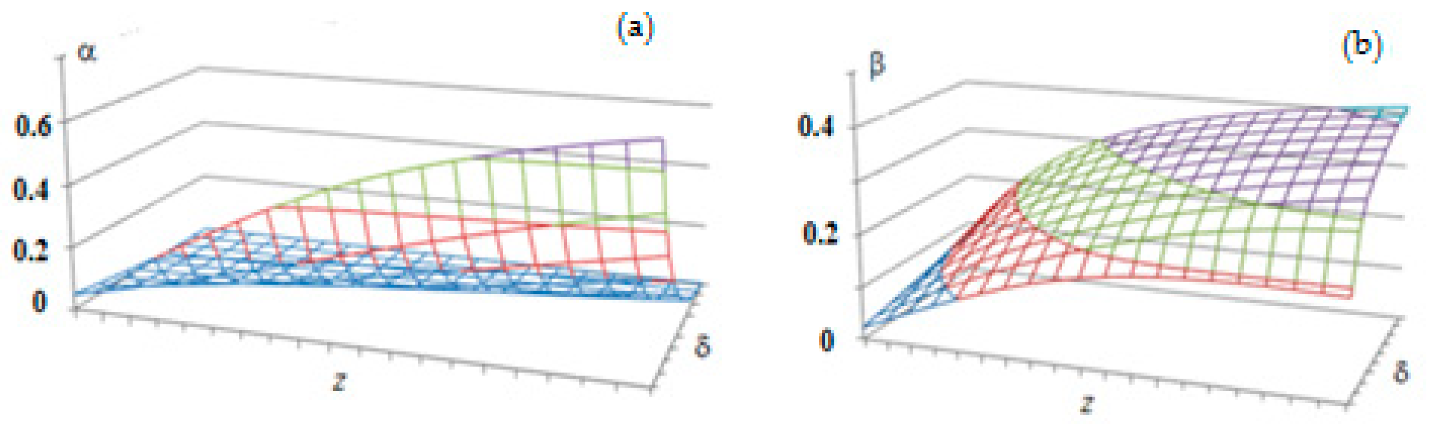
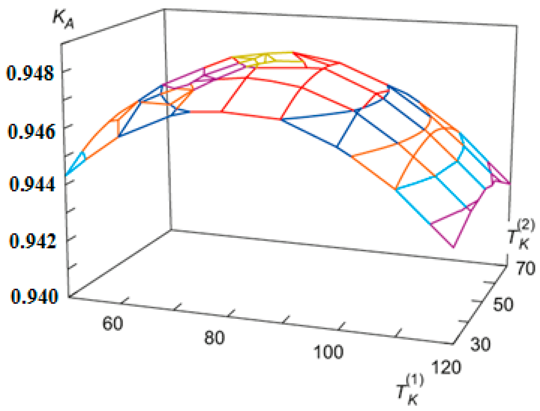
On the basis of solving a series of problems on the extremum of a function of several variables (21), the influence of the TIBV $T_K^{(j)}$ of the CTS from different degradation groups and the relative tolerances on controlled parameters ${\delta }_{}^{(j)}$ on the readiness coefficient are analyzed $K_A$.

Consider the effect of the duration of the TIBV on the readiness coefficient $K_A$. Let us fix all the arguments (21), with the exception of three: $T_K^{\left(i\right)},i=1,2,3$. If we additionally, fix any two arguments $T_K^{(i)}$ out of three, for example $T_K^{\left(2\right)}=C_{T_K}^{\left(2\right)*}$, $T_K^{\left(3\right)}=C_{T_K}^{\left(3\right)*}$, then the dependence of function (21) on the remaining argument $T_K^{(1)}$ will have the form given in [2]: convex upwards with a single maximum.

An asterisk in the upper index means that the corresponding value is set and fixed. If one of the three arguments is fixed in function (21) (for example, $T_K^{\left(3\right)}=C_{T_K}^{\left(3\right)*}$), then the readiness coefficient curve $K_A$, as well as the functions of the other two arguments, $T_K^{(1)}$ and $T_K^{(2)}$, will be convex upwards (Figure 11). The maximum of the readiness coefficient $K_A$ will be reached at a single internal point in the parameter plane, $T_K^{(1)}\times T_K^{(2)}$. The dependences of the readiness coefficient $K_A$ on the frequency of the control for the first and third groups, and for the second and third groups of degradation, have a similar form.

Optimization (21) for three groups of degradation showed that the characteristic ratio of the TIBV durations is 80:45:30, thus, the higher the degradation group, the more often CTS verifications are required.

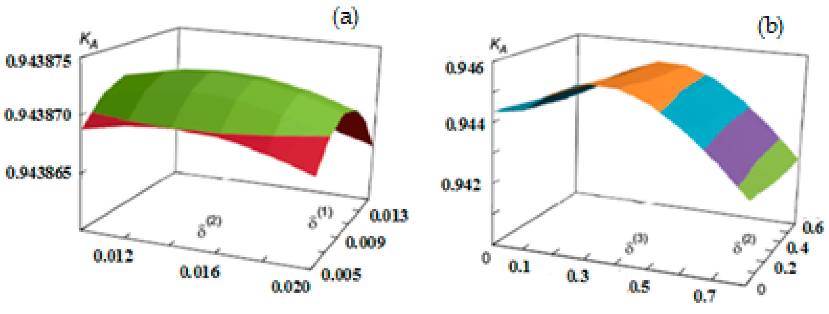
Consider the effect of the relative operating tolerances ${\mathsf{\delta }}^{\left(j\right)},j=1,2,3$ on $K_A$. Similarly to the above, we fix all the arguments (21), with the exception of three ${\mathsf{\delta }}^{\left(j\right)},j=1,2,3$. Then, the dependence of the readiness coefficient $K_A$ on relative operational tolerances is similar to its dependence on the TIBV, $T_K^{\left(i\right)},i=1,2,3$.

The calculations have shown that the general form of dependence $K_A$ on two tolerances, at a fixed value of the third tolerance, has the form of surfaces shown in Figure 12. The surface of the readiness coefficient $K_A$ as a function of two arguments will be convex upwards, where the maximum is reached at a single internal point in the parameter plane, ${\mathsf{\delta }}_{}^{(1)}\times {\mathsf{\delta }}_{}^{(2)}$, ${\mathsf{\delta }}_{}^{(1)}\times {\mathsf{\delta }}_{}^{(3)}$ or ${\mathsf{\delta }}_{}^{(2)}\times {\mathsf{\delta }}_{}^{(3)}$. Optimization of the $K_A$ of three relative tolerances simultaneously showed that their characteristic ratio is 0.07:0.09:0.13, thus, the higher the degradation group, the greater the tolerance.

The study of the joint dependence $K_A$ on the TIBV and tolerances showed that the maximum of the function of six variables is achieved at a single internal point of a set of parameters, $T_K^{(1)}\times T_K^{(2)}\times T_K^{(3)}\times {\mathsf{\delta }}_{}^{(1)}\times {\mathsf{\delta }}_{}^{(2)}\times {\mathsf{\delta }}_{}^{(3)}$. The optimal values of the arguments were: $T_K^{(1)}=81.59$, $T_K^{(2)}=50.46$, $T_K^{(3)}=32.55$, ${\delta }_{}^{(1)}=0.072$, ${\delta }_{}^{(2)}=0.0872$ and ${\delta }_{}^{(3)}=0.128$. At the same time, the optimal values of the probabilities of false and undetected failures were: ${\alpha }_{}^{(1)}=0.227$, ${\alpha }_{}^{(2)}=0.267$, ${\alpha }_{}^{(3)}=0.347$, ${\beta }_{}^{(1)}=0.171$, ${\beta }_{}^{(2)}=0.222$ and ${\beta }_{}^{(3)}=0.323$. The calculations have shown that with an increase in the number of the degradation group, the TIBV decreases, the tolerances for controlled parameters and the probabilities of false and undetected failures increase. The probabilities of false failures slightly exceed the corresponding probabilities of undetected failures for each degradation group.

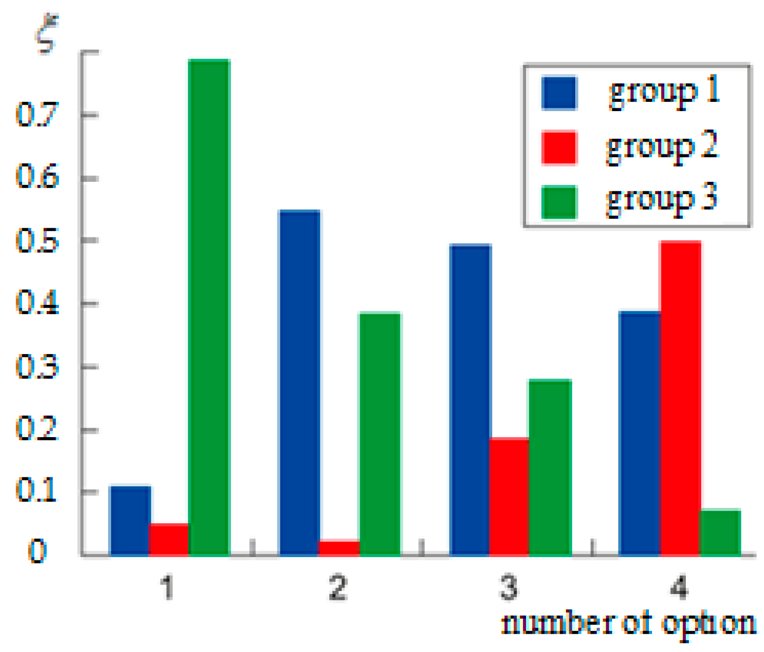
We describe the results of a study on the stationary distribution of the CTS samples in different degradation groups, depending on the rate of degradation processes. The rate of degradation is determined using transition probabilities ${\chi }_{}^{(i)}$, ${\eta }_{}^{(i)}$. The lower the corresponding probability, the slower the degradation processes proceed. Four variants differing in the rate of degradation were investigated: ${\eta }_{}^{(1)}=0.25$, ${\chi }_{}^{(1)}=0.2$, ${\eta }_{}^{(2)}=0.35$, ${\chi }_{}^{(2)}=0.3$ (option 1); ${\eta }_{}^{(1)}=0.025$, ${\chi }_{}^{(1)}=0.02$, ${\eta }_{}^{(2)}=0.35$, ${\chi }_{}^{(2)}=0.3$ (option 2); ${\eta }_{}^{(1)}=0.025$, ${\chi }_{}^{(1)}=0.02$, ${\eta }_{}^{(2)}=0.035$, ${\chi }_{}^{(2)}=0.03$ (option 3); and ${\eta }_{}^{(1)}=0.025$, ${\chi }_{}^{(1)}=0.02$; ${\eta }_{}^{(2)}=0.035$, ${\chi }_{}^{(2)}=0.003$ (option 4). Note that the variants are arranged in order of decreasing degradation rate. The distribution of the proportion of working samples of the CTS by degradation groups at different values of these parameters is shown in Figure 13.

The probability of the CTS staying in the first degradation group for option 2 is about 5.5 times higher compared to option 1. At the same time, the ratio of the probability of being in the third group compared to the probability of being in the first group remains approximately the same.

The probability of the CTS staying in the first degradation group monotonically decreases, and the probability of being in the second group monotonically increases with sequential consideration of options from 2 to 4.

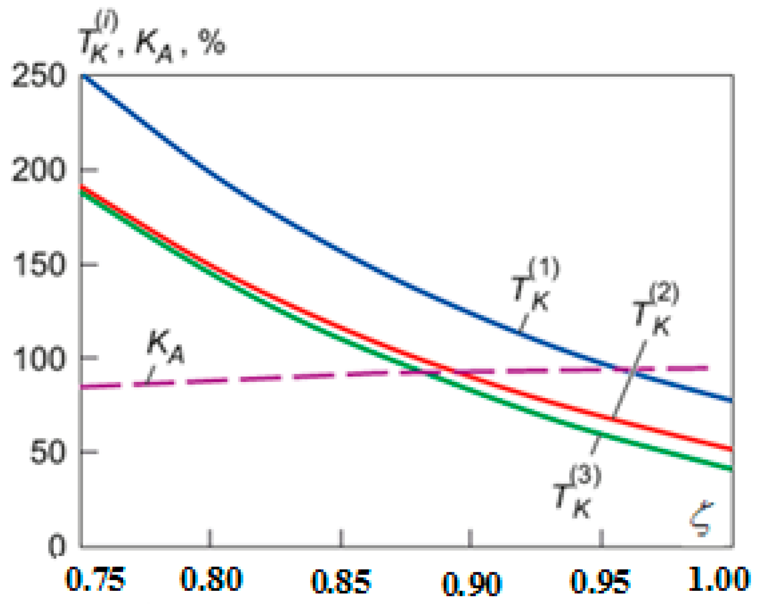
Next, we investigate the dependence $K_A$ on the total production capacity of the metrological units in which the MI and CTS are verified and checked. The production capacity of a metrological unit may be temporarily limited for one reason or another. The specified restriction was set in the form of an inequality, ${\displaystyle \sum _j{\mathsf{\pi }}^{\left(j\right)}{\mathsf{\psi }}^{\left(j\right)}}\le C^{\left(\mathsf{\pi }\right)*}$, where $C^{\left(\mathsf{\pi }\right)*}$ is the conditional production capacity of the metrological unit, and the problem of conditional optimization was solved. In Figure 14 the dependences of the TIBV on the total conditional production capacity $\zeta$ of the metrological units and the readiness coefficient corresponding to these intervals (in percent) are presented.

If the production capacities of the metrological division do not allow for the checking of the required number of CTS, then it is possible to operate a fleet of CTS with increased TIBV. With a decrease in the production capacity of the metrological unit from 100% to 75%, the readiness coefficient $K_A$ decreases from 0.9514 to 0.8402.

5. Results

A set of interrelated mathematical models of the processes of operation, renewal and degradation of a fleet of CTS with metrological support was developed. The basis of the developed set of models consists of:

−

A basic model of the CTS operation;

−

A set of CTS operation models, having different levels of degradation (for different levels of CTS degradation a different number of system states and different variants of system maintenance are used);

−

A model of false failures and undetected failures;

−

A model of CTS fleet renewal, including such renewal methods as the purchase of new CTS samples, the modernization of existing CTS samples and the development of new promising CTS samples;

−

A functional dependence model of the CTS availability factor on a number of technical parameters, organizational and technical parameters, and technological parameters of the CTS belonging to different degradation groups and different methods of CTS stock renewal.

On the basis of the set of interrelated mathematical models presented in the article, the software for modeling the processes of operation, renewal and degradation of the fleet of CTS with metrological support was developed.

6. Discussions

The models developed and implemented as software allow for the parametrical optimization of the processes of CTS fleet functioning for a number of parameters, including metrological parameters, organizational and technical parameters, and technical parameters.

If in practice it is impossible to provide the optimal TIBV values or tolerances for the controlled parameters for some degradation groups, then for these groups the “possible” values of the TIBV and tolerances for the controlled parameters should be established, and the developed models should be used for calculation.

The developed set of models include a model for calculating the probabilities of false failures and undetected failures, for use in cases where the measured parameter and measurement error have a normal distribution law. The set of models developed in the article can also be used for different distribution laws of the measured parameter and measurement error: analytical defined laws, statistical defined laws or analytical and statistical distribution laws.

The constructed functional dependences of the availability factor on metrological, technical, organizational, technical and technological parameters have a smooth character, which makes it possible to effectively investigate the extreme properties of the availability factor using standard gradient methods.

7. Conclusions

Thus, the research goal has been achieved: a set of interrelated models has been developed, which solves the current need for end-to-end modeling of all the main stages of the life cycle of the CTS fleet. The developed set of models makes it possible to adequately simulate large CTS fleets, including those incorporating up to several hundreds of thousands of CTS samples.

The developed set of interrelated models allows:

−

Management of the process of development of CTS fleets;

−

Optimization of the processes of CTS fleet functioning;

−

Identification of problematic issues in the development of CTS fleet and the formation of strategies for CTS fleet development in the presence of various constraints;

−

The solving of the problem of conditional optimization in the presence of constraints on the technological parameters of the CTS fleet development (with constraints on part of the arguments of the availability factor function);

−

Calculation of the technological and technical–economic parameters of the CTS fleet functioning and development;

−

Evaluation of the risks associated with false and undetected failures, as well as the risks associated with CTS degradation;

A set of models is used in the Main Scientific Metrology Center:

−

To classify the designed CTS in order to establish the requirements for their metrological support;

−

When developing plans for medium-term and long-term development of the CTS fleet.

A set of models and software can be used by design organizations involved in the development of modern and advanced CTS with metrological support.

8. Future Works

At present, a set of models continues to develop in the direction of development and replenishment with models of CTS fleet maintenance; namely, models of workplaces for the verification of MI, taking into account the priorities of the MI samples coming for verification [27,28], as well as models of CTS fleet functioning under such modes of functioning as the mode of high readiness for use, the mode of use in extreme conditions, etc.