The Qualitative Analysis of Host–Parasitoid Model with Inclusion of Spatial Refuge Effect

Abstract

The objective of this work was to investigate the dynamics of host–parasitoid model with spatial refuge effect. For this, two discrete host–parasitoid models were considered under spatial refuge effect. Suppose that a constant population of hosts may seek refuge and protection from an attack of parasitoids. We found the parametric factors affecting the existence of the equilibrium points and uniqueness of equilibrium points. A local stability analysis of host–parasitoid models was also carried out. Bifurcation theory was used to observe that the host–parasitoid models undergo Neimark–Sacker bifurcation. The effect of the existence of constant refuge effect on the local stability and bifurcation of models was also explored. Hybrid chaos control methodology was used to control the chaotic behavior of model. In addition, numerical simulations, bifurcation diagrams, and phase portraits of the models are also presented.

1. Introduction

The host–parasitoid model in discrete dynamical systems is a way to describe the population dynamics of a host species and its parasitoid species over discrete-time intervals. This model is based on a set of equations that describe how the populations of the two species change from one time step to the next. The model assumes that the populations of the host and parasitoid species are discrete, meaning they are represented by integers. A model that has secured appreciable recognition from both theoretical and experimental point of view is the host–parasitoid model. The host–parasitoid collaborations are the most accepted topics in mathematical biology as they are necessary to deal with the natural enemy of a pest or insect [1,2,3,4,5,6]. We observe that parasitoids are insect species whose larvae grow as parasites on further insect species. It has been discovered that larvae of parasitoids generally kill and sometimes paralyze its host. However, usually, mature parasitoid individuals are free-living insects. Moreover, parasitoids are characterized, in general, by insects that show one or more larval stages that parasite other arthropods, developing inside them and killing them before the end of their life cycle. Life cycles of parasitoids and their hosts are usually synched, e.g., hosts and parasitoids are univoltine (one generation per year) species. Discrete-time steps corresponding to generations are usually used in such models [7,8,9,10]. Parasitoids commonly include species of wasps, flies, beetles, and worms. On the other hand, a special case is where some preys are fully safe from attack of predators within a progressive or spatial refuge. Spatial refuges can take a variety of forms lying between two extremes, which are given as follows:

(i)

Where the constant ratio of the host populations is safe within refuge.

(ii)

Where the constant number is protected.

The most common among these are the constant proportion refuges. For example, flour moth caterpillars are protected from attack of parasitoids by the ichneumonid (Nemeritis canescen) when they are sufficiently deep in the flour medium to be out of reach of the parasitoid’s ovipositor. In this way, only a proportion of the host’s habitat is searched [11,12,13,14,15]. Before starting our discussion related to the mathematical modeling of host–parasitoid interaction under refuge effects, it is worthwhile to describe the pioneering contribution proposed by Nicholson and Bailey [16]. The mathematical model presented by Nicholson and Bailey is acknowledged as the Nicholson–Bailey (NB) model and is directed by the autonomous planar system of nonlinear difference equations as follows:

$$\begin{array}{l}{H}_{t+1}=r H_t exp\left(-a P_t\right) \\ P_{t+1}=c H_t \left(1-exp\left(-a P_t\right)\right)\end{array}$$

(1)

where $H_t$ and $P_t$ are state variables representing population concentrations of host and parasitoid at some instant $t$, respectively. Moreover, $r$ and $c$ are growth rates of host and parasitoid, respectively, and $a$ denotes the searching efficiency of parasitoids. Further investigation reveals that the NB model has trivial and interior (positive) fixed points. Moreover, a unique positive fixed equilibrium point occurs when $r>1$ and is always unstable, which contradicts the fact that the NB model is a noble descriptive of regular host–parasitoid interactions because most of these interactions are stable and do not possess any oscillatory behavior. Various attempts were made by numerous mathematicians and ecologists to formulate appropriate modifications to the classical NB model. One of these modifications is to introduce the refuge effect on the classical NB model. For this, we study two modifications proposed by Hassell in [17]:

Firstly, we consider a constant population of hosts, keeping in view the NB model, to examine the spatial refuge effect. A fraction of host specie $\alpha$ is accessible to the parasitoid specie in every single generation. Consequently, $\left(1-\alpha \right)$ is the population within spatial refuge. This is represented by the following model.

$$\begin{array}{l}{H}_{t+1}=r\left(1-\alpha \right) H_t+r\alpha H_t exp\left(-a P_t\right)\\ P_{t+1}=\alpha H_t \left(1-exp\left(-a P_t\right)\right) \end{array}$$

(2)

Relative proportions lead to stability under refuges but large areas of parameter space remain for unstable equilibrium (too few hosts within the refuge) or no equilibrium at all (too many hosts within the refuge).

Secondly, consider constant number refuge, where $H_0$ hosts are always protected, and we obtain:

$$\begin{array}{l}{H}_{t+1}=r{H}_0+r\left(H_t-H_0\right)exp\left(-a P_t\right)\\ P_{t+1}=\left(H_t-H_0\right) \left(1-exp\left(-a P_t\right)\right) \end{array}$$

(3)

The spatial refuge can play an important role in the dynamics of the model, potentially leading to the persistence of the host population even in the presence of high parasitoid attack rates.

The main contribution of this article is to explore the dynamics of systems (2) and (3). It would be beneficial first to clarify certain fundamental concepts and mathematical outcomes pertaining to our primary inquiry, prior to delving into an all-encompassing examination of the qualitative behaviors exhibited by these systems. Since systems (2) and (3) are planar discrete-time models governed by autonomous nonlinear systems of difference equations, therefore we start with the dynamical behavior of the general planar systems. The key investigations of the manuscript are synopsized in the following discussion.

2. Stability Analysis around Equilibria

In order to obtain the equilibrium points of the system (2), we transform the system as follows.

$$\begin{array}{l}{x}_{n+1}=r\left(1-p\right)x_n+rp{x}_n{e}^{-a{y}_n},\\ y_{n+1}=p{x}_n\left(1-e^{-a{y}_n}\right). \end{array} , 0<p<1.$$

Consider map:

$$\left(\begin{array}{c}x\\ y\end{array}\right)\to \left(\begin{array}{c}r\left(1-p\right)x+rpx{e}^{-ay}\\ px\left(1-e^{-ay}\right)\end{array}\right)$$

Here we introduce,

$$f\left(x,y\right)=r\left(1-p\right)x+rpx{e}^{-ay}$$

$$g\left(x,y\right)=px\left(1-e^{-ay}\right)$$

The equilibria $O\left(0,0\right)$ and $\Omega \left(x^{\star }, y^{\star }\right)$ are obtained, where $x^{\star }=\frac{1}{a}\frac{\ln \frac{rp}{1-r\left(1-p\right)}}{r-1}, y^{\star }=\frac{1}{a}\ln \frac{rp}{1-r\left(1-p\right)}, 1<r<\frac{1}{1-p}$, $p\in \left(0,1\right)$. To demonstrate the stability (local) analysis of a biologically suitable equilibrium, the following lemma is the best interpretation [18,19].

Lemma 1.

Let $\mathit{F}\left(\mathit{\lambda }\right)={\mathit{\lambda }}^{\mathbf{2}}-Trace\left(\mathit{J}\right) \mathit{\lambda }+Determinant\left(J\right).$ This is called the characteristic equation of variational matrix $\mathit{J}$ and ${\mathit{\lambda }}_{\mathbf{1}}$ and ${\mathit{\lambda }}_{\mathbf{2}}$ are the eigenvalues of this equation. Now, a unique positive equilibrium point is termed as a sink if the absolute values of ${\mathit{\lambda }}_{\mathbf{1}}$ and${\mathit{\lambda }}_{\mathbf{2}}$ is one. Consequently, a sink is always a local asymptotic stable equilibrium point. When $|{\mathit{\lambda }}_{\mathbf{1}}| > \mathbf{1}$ along with $|{\mathit{\lambda }}_{\mathbf{2}}| >\mathbf{1}$, the equilibrium point is known as a repeller; thus, we always have a source which is unstable. When $\left|{\mathit{\lambda }}_{\mathbf{1}}\right|<\mathbf{1}$ and $\left|{\mathit{\lambda }}_{\mathbf{2}}\right|>\mathbf{1}$ or $\left|{\mathit{\lambda }}_{\mathbf{1}}\right|>\mathbf{1}$ and $\left|{\mathit{\lambda }}_{\mathbf{2}}\right|<\mathbf{1}$, then the equilibrium point is called a saddle and it is always unstable. When the absolute value of either of ${\mathit{\lambda }}_{\mathbf{1}}$ and ${\mathit{\lambda }}_{\mathbf{2}}$ is one, then we get a non-hyperbolic equilibrium point.

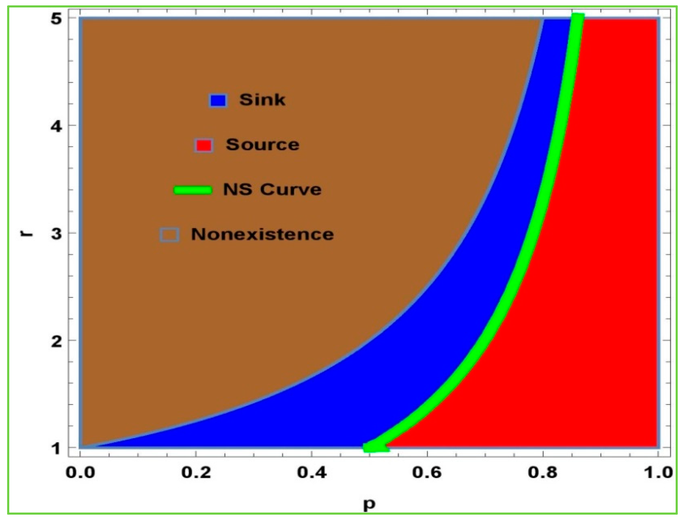
Taking into account the positivity and existence of model (2) at $\Omega \left(x^{\star }, y^{\star }\right)$, one can take $r>1$. In Figure 1, the blue region shows the sink, and the red region shows the source. Moreover, the yellow region shows the Hopf bifurcation. The nonexistence of the model (2) is represented by the white area. Thus, the Jacobian matrix at $\Omega \left(x^{\star }, y^{\star }\right)$ is:

$$J\left(x^{\star }, y^{\star }\right)=\left(\begin{array}{cc}1& \frac{r\left(-1+r-pr\right)\ln \left(\frac{pr}{1+\left(-1+p\right)r}\right)}{-1+r}\\ \frac{-1+r}{r}& \frac{\left(1+\left(-1+p\right)r\right)\ln \left(\frac{pr}{1+\left(-1+p\right)r}\right)}{-1+r}\end{array}\right)$$

and the characteristic polynomial is given as:

$$F\left(\lambda \right)={\lambda }^2-\left(1+\frac{\left(1+\left(-1+p\right)r\right)\ln \left(\frac{pr}{1+\left(-1+p\right)r}\right)}{-1+r}\right)\lambda +\frac{r\left(1+\left(-1+p\right)r\right)\ln \left(\frac{pr}{1+\left(-1+p\right)r}\right)}{-1+r}.$$

By simple calculations, we obtain:

$$F\left(1\right)=\left(1+\left(-1+p\right)r\right)\ln \left[\frac{pr}{1+\left(-1+p\right)r}\right]>0$$

$$F\left(-1\right)=2+\frac{\left(1+r\right)\left(1+\left(-1+p\right)r\right)\ln \left[\frac{pr}{1+\left(-1+p\right)r}\right]}{-1+r}$$

and

$$F\left(0\right)=\frac{r\left(1+\left(p-1\right)r\right)\ln \left(\frac{pr}{1+\left(p-1\right)r}\right)}{r-1}.$$

Now, suppose ${\lambda }_1,{\lambda }_1$ be two roots of the system of Equations (2), then the positive equilibrium point is given by $\Omega \left(x^{\star }, y^{\star }\right)=\left(\frac{1}{a}\frac{\ln \frac{rp}{1-r\left(1-p\right)}}{r-1}, \frac{1}{a}\ln \frac{rp}{1-r\left(1-p\right)}\right).$According to the lemma 1, system (2) has the following conditions related to the stability analysis.

• The equilibrium point $\Omega \left(x^{\star }, y^{\star }\right)$ is a sink, if and only if $F\left(-1\right)>0$ and $F\left(0\right)<1$.
• The equilibrium point $\Omega \left(x^{\star }, y^{\star }\right)$ is a source, if and only if $F\left(-1\right)>0$ and $F\left(0\right)>1$.
• The equilibrium point $\Omega \left(x^{\star }, y^{\star }\right)$ is a saddle point, if and only if $F\left(-1\right)<0$.

Now, we consider the dynamics of model (3) by replacing $H$ and $P$ with $x$ and $y$. It is clear that system (3) has two equilibrium points, the trivial equilibrium point (0, 0) and the unique positive equilibrium point $\left(x^{\star }, y^{\star }\right)=\left(x_0+\frac{y^{\star }}{1-e^{-a{y}^{\star }}},\frac{1}{a}\ln \left|\frac{r\left(x^{\star }-x_0\right)}{x^{\star }-r{x}_0}\right| \right)$, with $r>1,$and $r{x}_0<x^{\star }.$

The Jacobian matrix computed at $\left(0, 0\right)$ is:

$$J\left(0, 0\right)=\left(\begin{array}{ll}r& ar{x}_0\\ 0& -a{x}_0\end{array}\right).$$

Clearly, $\left(0, 0\right)$ is a sink if and only if $0<r<1$ and a saddle if $r>1$.

The Jacobian matrix at the interior steady state $\left(x^{\star }, y^{\star }\right)$ is calculated as:

$$J \left(x^{\star }, y^{\star }\right)=\left(\begin{array}{cc}\frac{x^{\star }-r{x}_0}{x^{\star }-x_0}& -\frac{a{e}^{a{y}^{\star }}\left(x^{\star }-r{x}_0\right)y^{\star }}{\left(e^{a{y}^{\star }}-1\right)\left(x^{\star }-x_0\right)}\\ \frac{\left(r-1\right)x}{r\left(x^{\star }-x_0\right)}& \frac{a\left(1+\frac{1}{e^{a{y}^{\star }}-1}\right)\left(x^{\star }-r{x}_0\right)y^{\star }}{r\left(x^{\star }-x_0\right)}\end{array}\right)$$

and the characteristic polynomial is given by:

$$F\left(\lambda \right)={\lambda }^2-\left(\frac{\left(x^{\star }-r{x}_0\right)\left(e^{a{y}^{\star }}\left(r+ay\right)-r\right)}{\left(e^{a{y}^{\star }}-1\right)r\left(x^{\star }-x_0\right)}\right)\lambda +\frac{a{e}^{a{y}^{\star }}\left(x^{\star }-r{x}_0\right)y^{\star }}{\left(e^{a{y}^{\star }}-1\right)\left(x^{\star }-x_0\right)}.$$

By simple calculations, we obtain:

$$\{\begin{array}{l}F\left(-1\right)=\frac{r\left(x_0+r{x}_0-2x^{\star }\right)-e^{a{y}^{\star }}\left(r\left(x_0+r{x}_0-2x^{\star }\right)+a\left(1+r\right)\left(r{x}_0-x^{\star }\right)y^{\star }\right)}{\left(e^{a{y}^{\star }}-1\right)r\left(x^{\star }-x_0\right)}\\ F\left(1\right)=\frac{\left(r-1\right)\left(e^{a{y}^{\star }}\left(r{x}_0+a\left(x^{\star }-r{x}_0\right)y^{\star }\right)-r{x}_0\right)}{\left(e^{a{y}^{\star }}-1\right)r\left(x^{\star }-x_0\right)}>0\\ F\left(0\right)=\frac{a{e}^{a{y}^{\star }}\left(x^{\star }-r{x}_0\right)y^{\star }}{\left(e^{a{y}^{\star }}-1\right)\left(x^{\star }-x_0\right)}.\end{array}$$

From the above mathematical computations, we deduced the following results:

• The unique steady-state $\left(x^{\star }, y^{\star }\right)$ is locally asymptotically stable if and only if:

  $$\frac{a\left(1+r\right)\left(r{x}_0-x^{\star }\right)y^{\star }}{r\left(x_0+r{x}_0-2x^{\star }\right)}<e^{-a{y}^{\star }}-1 \mathrm{and} \frac{a\left(x^{\star }-r{x}_0\right)y^{\star }}{\left(x^{\star }-x_0\right)}<1-e^{-a{y}^{\star }} .$$
• The unique steady-state $\left(x^{\star }, y^{\star }\right)$ is unstable if and only if:

  $$1+\frac{a\left(1+r\right)\left(r{x}_0-x^{\star }\right)y^{\star }}{r\left(x_0+r{x}_0-2x^{\star }\right)}<e^{-a{y}^{\star }} \mathrm{and} \frac{a\left(x^{\star }-r{x}_0\right)y^{\star }}{\left(x^{\star }-x_0\right)}>\frac{e^{a{y}^{\star }}-1}{e^{a{y}^{\star }}} .$$
• The unique steady-state $\left(x^{\star }, y^{\star }\right)$ is saddle if and only if:

  $$e^{-a{y}^{\star }}-1<\frac{a\left(1+r\right)\left(r{x}_0-x^{\star }\right)y^{\star }}{r\left(x_0+r{x}_0-2x^{\star }\right)}.$$
• The eigenvalues of the characteristic polynomial are complex conjugate with magnitude 1, if and only if:

  $$\left|\frac{\left(x^{\star }-r{x}_0\right)\left(e^{a{y}^{\star }}\left(r+ay\right)-r\right)}{\left(e^{a{y}^{\star }}-1\right)r\left(x^{\star }-x_0\right)}\right|<2,$$

  $$r=\frac{e^{-a{y}^{\star }}\left(x^{\star }-x_0+e^{a{y}^{\star }}\left(x_0+x^{\star }\left(a{y}^{\star }-1\right)\right)\right)}{a{x}_0{y}^{\star }}.$$

3. Neimark–Sacker Bifurcation in Model (2)

Now, we study the presence and trajectory of the Neimark–Sacker bifurcation for the unique positive equilibrium point $\Omega \left(x^{\star }, y^{\star }\right)$ of model (2). We must find sufficient conditions for the Neimark–Sacker bifurcation. The interior unique positive equilibrium point $\Omega \left(x^{\star }, y^{\star }\right)$ should be non-hyperbolic for the existence of Neimark–Sacker bifurcation, such that the variational matrix calculated at this point has two complex conjugate eigenvalues with an absolute value equal to one. Discrete-time models corresponding to population can also be investigated it the same way [20,21,22]. The conditions that determine the limitations for the existence of the Neimark-Sacker bifurcation are as follows:

$$F\left(0\right)=\frac{r\left(1+\left(-1+p\right)r\right)\ln \left[\frac{pr}{1+\left(-1+p\right)r}\right]}{-1+r}=1,$$

or

$$\ln \left[\frac{pr}{1+\left(-1+p\right)r}\right]=\frac{\left(-1+r\right)}{r\left(1+\left(-1+p\right)r\right)}$$

and

$$\left|\left(1+\frac{\left(1+\left(-1+p\right)r\right)\ln [\frac{pr}{1+\left(-1+p\right)r}]}{-1+r}\right)\right|<2.$$

Suppose that ${\Omega }_{NS}=\left\{\left(a,r,p\right)Є{ℝ}^3:r\equiv r_0,\left|A\right|<2\right\}$, then there is change of parameters in a small neighborhood of ${\Omega }_{NS}$, where ${\Omega }_{NS}$ produces the Neimark–Sacker bifurcation for the positive equilibrium point of system (2). The following two-dimensional map expresses the system of Equation (2) as:

$$\tilde{r}\left(\begin{array}{c}X\\ Y\end{array}\right)\to \left(\begin{array}{c}r\left(1-p\right)X+rpX{e}^{-aY}\\ pX\left(1-e^{-aY}\right)\end{array}\right).$$

Let $\tilde{r}$ indicate the bifurcating parameter, and then the perturbed mapping of the above system is as follows:

$$\left(\begin{array}{c}X\\ Y\end{array}\right)\to \left(\begin{array}{c}R\left(\left(1-p\right)X+pX{e}^{-aY}\right)\\ pX\left(1-e^{-aY}\right)\end{array}\right)$$

where $R=r_1+\tilde{r}$ and the small perturbation parameter is denoted by $\left|\tilde{r} \right|<<1.$ Where $x=X-\frac{1}{a}\frac{\ln \frac{rp}{1-r\left(1-p\right)}}{r-1}$ and $y=Y-\frac{1}{a}\ln \frac{rp}{1-r\left(1-p\right)}$. Then from above map, we have

$$\left(\begin{array}{c}X\\ Y\end{array}\right)\to \left(\begin{array}{cc}{m}_{11}& m_{12}\\ m_{21}& m_{22}\end{array}\right)\left(\begin{array}{c}x\\ y\end{array}\right)+\left(\begin{array}{c}{f}_1\left(x,y\right)\\ f_2\left(x,y\right)\end{array}\right),$$

where

$$f_1\left(x,y\right)=m_{13}{x}^2+m_{14}xy+m_{15}{x}^{2}y+O\left({\left(\left|x\right|+\left|y\right|\right)}^4\right),$$

$$f_2\left(x,y\right)=m_{23}{x}^2+m_{24}xy+m_{25}{x}^{2}y+O\left({\left(\left|x\right|+\left|y\right|\right)}^4\right),$$

$$m_{11}=1-\frac{1}{R}+\frac{\ln \left[\frac{pR}{1+\left(-1+p\right)R}\right]}{a}; m_{12}=\frac{e^{-a}\left(-1+\left(1+\left(-1+e^a\right)p\right)R\right)\ln \left[\frac{pR}{1+\left(-1+p\right)r}\right]}{a\left(-1+r\right)} ;$$

$$m_{14}=p\left(1+\frac{e^{-a}\left(-1+r-pR\right)}{pR}\right)\left(1+\frac{R\ln \left[\frac{pR}{1+\left(-1+p\right)R}\right]}{a\left(-1+R\right)}\right); m_{21}=1-\frac{1}{R}+\frac{\ln \left[\frac{pR}{1+\left(-1+p\right)R}\right]}{a};$$

$$m_{22}=\frac{e^{-a}\left(-1+\left(1+\left(-1+e^a\right)p\right)R\right)\ln \left[\frac{pR}{1+\left(-1+p\right)R}\right]}{a\left(-1+R\right)}; m_{24}=p\left(1+\frac{e^{-a}\left(-1+R-pR\right)}{pR}\right)\left(1+\frac{R\ln \left[\frac{pR}{1+\left(-1+p\right)R}\right]}{a\left(-1+R\right)}\right);$$

$$m_{25}=p\left(1+\frac{e^{-a}\left(-1+R-pR\right)}{pR}\right)2+\frac{R\ln \left[\frac{pR}{1+\left(-1+p\right)R}\right]}{a\left(-1+R\right)}.$$

The characteristic equation for the Jacobian matrix at equilibrium point (0, 0) is

$${\lambda }^2-A\left(\tilde{r}\right)\lambda +B\left(\tilde{r}\right)=0.$$

Since $\left(a,r,p\right)Є{\Omega }_{NS}$. Hence, the complex conjugate roots can be written as

$${\lambda }_1=\frac{A\left(\tilde{r}\right)-i\sqrt{4B\left(\tilde{r}\right)-{\left(A\left(\tilde{r}\right)\right)}^2}}{2}, {\lambda }_2=\frac{A\left(\tilde{r}\right)+i\sqrt{4B\left(\tilde{r}\right)-{\left(A\left(\tilde{r}\right)\right)}^2}}{2}.$$

where

$$A\left(\tilde{r}\right)=1+\frac{\left(1+\left(-1+p\right)R\right)\ln \left[\frac{pR}{1+\left(-1+p\right)R}\right]}{-1+R}$$

and

$$B\left(\tilde{r}\right)=\frac{R\left(1+\left(p-1\right)R\right)\ln \left[\frac{pR}{1+\left(p-1\right)R}\right]}{R-1}.$$

Thus,

$$\left|{\lambda }_1\right|=\left|{\lambda }_2\right|=\sqrt{\frac{R\left(1+\left(p-1\right)R\right)\ln \left[\frac{pR}{1+\left(p-1\right)R}\right]}{R-1}}.$$

Now, to obtain the non-degeneracy conditions, we observe that

$${\left(\frac{d\left|{\lambda }_1\right|}{d\tilde{r}}\right)}_{\tilde{r}=0}={\left(\frac{d\left|{\lambda }_2\right|}{d\tilde{r}}\right)}_{\tilde{r}=0}\ne 0.$$

Moreover, we have $-2<A\left(0\right)<2$ because $\left(\alpha ,\beta ,r_1\right)\in {\Omega }_{NS}$. Now, consider that

$$A\left(0\right)=1+\frac{\left(1+\left(-1+p\right)r_1\right)\ln \left[\frac{p{r}_1}{1+\left(-1+p\right)r_1}\right]}{-1+r_1}.$$

Hence, we observe that $A\left(0\right)\ne 0$ and $A\left(0\right)\ne -1$, that is consider $A\left(0\right)\ne \pm 2,0,-1.$

$$\begin{array}{c}1+\frac{\left(1+\left(-1+p\right)r_1\right)\ln \left[\frac{p{r}_1}{1+\left(-1+p\right)r_1}\right]}{-1+r_1}\ne -1\\ 1+\frac{\left(1+\left(-1+p\right)r_1\right)\ln \left[\frac{p{r}_1}{1+\left(-1+p\right)r_1}\right]}{-1+r_1}\ne 0.\end{array}\}$$

(4)

Moreover, $B\left(0\right)=\frac{r\left(1+\left(-1+p\right)r_1\right)\ln \left[\frac{p{r}_1}{1+\left(-1+p\right)r_1}\right]}{-1+r_1}.$

Make sure that $A\left(0\right)\ne \pm 2, 0,-1$, and as a result we have ${\lambda }_1{}^m$,${\lambda }_2{}^m\ne 1,2,3,4$ when $\tilde{r}=0$. Henceforth, the roots of the system cannot exist within the intersection of the circle with a unit radius with the synchronized axes if $\tilde{r}=0$. To obtain the normal form when $\tilde{r}=0$, we assume that $k=\frac{A\left(0\right)}{2}$ at $\omega =\frac{\sqrt{4B\left(0\right)-A{\left(0\right)}^2}}{2}.$ Thus,

$$k=\frac{1}{2}\left[1+\frac{\left(1+\left(-1+p\right)r_1\right)\ln \left(\frac{p{r}_1}{1+\left(-1+p\right)r_1}\right)}{r_1-1}\right]$$

and

$$\omega =\frac{\sqrt{4\frac{r\left(1+\left(-1+p\right)r_1\right)\ln \left[\frac{p{r}_1}{1+\left(-1+p\right)r_1}\right]}{-1+r_1}-{\left(1+\frac{\left(1+\left(-1+p\right)r_1\right)\ln \left[\frac{p{r}_1}{1+\left(-1+p\right)r_1}\right]}{-1+r_1}\right)}^2}}{2}.$$

Furthermore, considering the following transformation:

$$\left(\begin{array}{c}x\\ y\end{array}\right)\to \left(\begin{array}{cc}{m}_{12}& 0\\ k-m_{11}& -\omega \end{array}\right)\left(\begin{array}{c}u\\ \nu \end{array}\right).$$

Under this transformation, our system can be written as:

$$\left(\begin{array}{c}x\\ y\end{array}\right)\to \left(\begin{array}{cc}k& -\omega \\ \omega & k\end{array}\right)\left(\begin{array}{c}u\\ \nu \end{array}\right)+\left(\begin{array}{c}\widetilde{f_1}\left(x,y\right)\\ \widetilde{f_2}\left(x,y\right)\end{array}\right).$$

$$\widetilde{f_1}\left(x,y\right)=\frac{m_{13}}{m_{12}}{x}^2+\frac{m_{14}}{m_{12}}xy+\frac{m_{15}}{m_{12}}{y}^2+O\left({\left(\left|u\right|+\left|v\right|\right)}^4\right)$$

$$\widetilde{f_2}\left(x,y\right)=\left(\frac{\left(k-m_{11}\right)m_{13}}{m_{12}\omega }-\frac{m_{23}}{\omega }\right)x^2+\left(\frac{\left(k-m_{11}\right)m_{14}}{m_{12}\omega }-\frac{m_{24}}{\omega }\right)xy+\left(\frac{\left(k-m_{11}\right)m_{15}}{m_{12}\omega }-\frac{m_{25}}{\omega }\right)y^2+O\left({\left(\left|u\right|+\left|v\right|\right)}^4\right).$$

$$x=m_{12}u \mathrm{and} y=\left(k-m_{11}\right)u-\omega v.$$

Then consider a real number as follow:

$$L_1={\left(\left[-Re\left(\frac{(1-2{\lambda }_{1){\lambda }_2{}^2}}{1-{\lambda }_1}{\tau }_{20}{\tau }_{11}\right)-\frac{1}{2}{\left|{\tau }_{11}\right|}^2-{\left|{\tau }_{02}\right|}^2+Re\left({\lambda }_2{\tau }_{21}\right)\right]\right)}_{\tilde{r}=0}.$$

where

$${\tau }_{20}=\frac{1}{8}\left[{\widetilde{f_1}}_{uu}-{\widetilde{f_1}}_{vv}+2{\widetilde{f_2}}_{uv}+i\left({\widetilde{f_2}}_{uu}-{\widetilde{f_2}}_{vv}-2{\widetilde{f_1}}_{uv}\right)\right],$$

$${\tau }_{11}=\frac{1}{4}\left[{\widetilde{f_1}}_{uu}+{\widetilde{f_1}}_{vv}+i\left({\widetilde{f_2}}_{uu}-{\widetilde{f_2}}_{vv}\right)\right],$$

$${\tau }_{02}=\frac{1}{8}\left[{\widetilde{f_1}}_{uu}-{\widetilde{f_1}}_{vv}-2{\widetilde{f_2}}_{uv}+i\left({\widetilde{f_2}}_{uu}-{\widetilde{f_2}}_{vv}+2{\widetilde{f_1}}_{uv}\right)\right],$$

$${\tau }_{21}=\frac{1}{16}\left[{\widetilde{f_1}}_{uuu}+{\widetilde{f_1}}_{uvv}+{\widetilde{f_2}}_{uuv}+{\widetilde{f_2}}_{vvv}+i\left({\widetilde{f_2}}_{uuu}+{\widetilde{f_2}}_{uvv}-{\widetilde{f_1}}_{uuv}-{\widetilde{f_1}}_{vvv}\right)\right].$$

After conducting the aforementioned detailed investigation, we have the following precise result:

Theorem 1.

Assume that (1) holds and $L_1\ne 0,$ then system (2) undergoes the Neimark–Sacker bifurcation at the unique positive equilibrium point $\Omega \left(x^{\star }, y^{\star }\right)$, when the parameter $r$ varies in a small neighborhood of $r_1.$ Furthermore, if $L_1<0,$ then an attracting invariant closed curve bifurcates from the equilibrium point for $r_1<r,$ and if $L_1>0,$ then a repelling invariant closed curve bifurcates from the equilibrium point for $r_1>r.$

4. Neimark–Sacker Bifurcation in Model (3)

The two-dimensional map for model (3) is defined as:

$$\tilde{r}\left(\begin{array}{c}X\\ Y\end{array}\right)\to \left(\begin{array}{c}R(X_0+\left(X-X_0\right)e^{-aY}\\ \left(X-X_0\right)\left(1-e^{-aY}\right)\end{array}\right).$$

Let $\tilde{r}$ represent the bifurcation parameter where $\left|\tilde{r}\right|\ll 1$, and then corresponding perturbed mapping of above system is stated as follows:

$$\left(\begin{array}{c}X\\ Y\end{array}\right)\to \left(\begin{array}{c}R\left(X_0+\left(X-X_0\right)e^{-aY}\right)\\ \left(X-X_0\right)\left(1-e^{-aY}\right)\end{array}\right),$$

where $R=r_2+\tilde{r}$ and the small perturbation parameter is denoted by $\left|\tilde{r} \right|<<1.$ Then afterwards, consider the transformations x = X − ${\rm Y}$ and y = Y − $\xi$, the above map implies that

$$\left(\begin{array}{c}X\\ Y\end{array}\right)\to \left(\begin{array}{cc}{a}_{11}& a_{12}\\ a_{21}& a_{22}\end{array}\right)\left(\begin{array}{c}x\\ y\end{array}\right)+\left(\begin{array}{c}{g}_1\left(x,y\right)\\ g_2\left(x,y\right)\end{array}\right),$$

where

$$g_1\left(x,y\right)=a_{13}{x}^2+a_{14}xy+a_{15}{x}^{2}y+O\left({\left(\left|x\right|+\left|y\right|\right)}^4\right),$$

$$g_2\left(x,y\right)=a_{23}{x}^2+a_{24}xy+a_{15}{x}^{2}y+O\left({\left(\left|x\right|+\left|y\right|\right)}^4\right).$$

$$a_{11}=R, a_{12}=-a{e}^{-aY}, a_{21}=1-e^{-aY}, a_{22}=a{e}^{-aY}\left(X-X_0\right), a_{24}=a{e}^{-aY}.$$

The characteristic equation for the Jacobian matrix at the equilibrium point (0, 0) is

$${\sigma }^2-A\left(\tilde{r}\right)\sigma +B\left(\tilde{r}\right)=0.$$

Since $\left(a,r,p\right)\in {\Omega }_{NS}$. Hence, the complex conjugate roots can be written as

$${\sigma }_{1,2}=\frac{A\left(\tilde{r}\right)\pm i\sqrt{4B\left(\tilde{r}\right)-{\left(A\left(\tilde{r}\right)\right)}^2}}{2}.$$

where

$$A\left(\tilde{r}\right)=e^{-ay}\left(R+a\left(x-x_0\right)\right)$$

$$B\left(\tilde{r}\right)=a{e}^{-ay}R\left(x-x_0\right).$$

Thus, $\left|{\sigma }_1\right|=\left|{\sigma }_2\right|=\sqrt{a{e}^{-ay}R\left(x-x_0\right)}.$ Now, for obtaining the non-degeneracy conditions, we have

$${\left(\frac{d\left|{\sigma }_1\right|}{dr}\right)}_{\tilde{r}=0}={\left(\frac{d\left|{\sigma }_2\right|}{dr}\right)}_{\tilde{r}=0}=4r_{2}a{e}^{-ay}\left(x-x_0\right)\ne 0.$$

Moreover, we have $-2<A\left(0\right)<2$ because $\left(\alpha ,\beta ,r_2\right)\in {\Omega }_{NS}$. Also, $A\left(0\right)=a{e}^{-ay}\left(x-x_0\right).$ Now, suppose that $A\left(0\right)\ne 0,-1$ that is,

$$\begin{array}{c}A\left(0\right)=e^{-ay}\left(r_2+a\left(x-x_0\right)\right)\ne 0 \\ A\left(0\right)=e^{-ay}\left(r_2+a\left(x-x_0\right)\right)\ne -1.\end{array}\}$$

(5)

To obtain the normal form at $\tilde{r}=0$, we assume that $k=\frac{A\left(0\right)}{2}$ at $\omega =\frac{\sqrt{4B\left(0\right)-A{\left(0\right)}^2}}{2},$ where

$$k=\frac{e^{-ay}\left(r_2+a\left(x-x_0\right)\right)}{2} \mathrm{and} \omega =\frac{\sqrt{4a{e}^{-ay}{r}_2\left(x-x_0\right)-{(e^{-ay}\left(r_2+a\left(x-x_0\right)\right))}^2}}{2}.$$

Furthermore, we consider the following transformation:

$$\left(\begin{array}{c}x\\ y\end{array}\right)\to \left(\begin{array}{cc}{a}_{12}& 0\\ k-a_{11}& -\omega \end{array}\right)\left(\begin{array}{c}u\\ \nu \end{array}\right).$$

Under this transformation, our system can be written as

$$\left(\begin{array}{c}x\\ y\end{array}\right)\to \left(\begin{array}{cc}k& -\omega \\ \omega & k\end{array}\right)\left(\begin{array}{c}u\\ \nu \end{array}\right)+\left(\begin{array}{c}\widetilde{f_3}\left(x,y\right)\\ \widetilde{f_4}\left(x,y\right)\end{array}\right).$$

where

$$\widetilde{f_3}\left(x,y\right)=\frac{a_{13}}{a_{12}}{x}^2+\frac{a_{14}}{a_{12}}xy+\frac{a_{15}}{a_{12}}{y}^2+O\left({\left(\left|u\right|+\left|v\right|\right)}^4\right).$$

$$\widetilde{f_4}\left(x,y\right)=\left(\frac{a_{13}}{a_{12}\omega }-\frac{a_{23}}{\omega }\right)x^2+\left(\frac{\left(k-a_{11}\right)a_{14}}{a_{12}\omega }-\frac{a_{24}}{\omega }\right)xy+\left(\frac{\left(k-a_{11}\right)a_{15}}{m_{12}\omega }-\frac{a_{25}}{\omega }\right)y^2+O\left({\left(\left|u\right|+\left|v\right|\right)}^4\right).$$

$x=a_{12}u$ and $y=\left(k-a_{11}\right)u-\omega v.$ Now, we consider a real number as follows:

$$L_2={\left(\left[-Re\left(\frac{(1-2{\sigma }_{1){\sigma }_2{}^2}}{1-{\sigma }_1}{\xi }_{20}{\xi }_{11}\right)-\frac{1}{2}{\left|{\xi }_{11}\right|}^2-{\left|{\xi }_{02}\right|}^2+Re\left({\sigma }_2{\xi }_{21}\right)\right]\right)}_{\tilde{r}=0}.$$

where

$${\xi }_{20}=\frac{1}{8}\left[{\widetilde{f_3}}_{uu}-{\widetilde{f_3}}_{vv}+2{\widetilde{f_4}}_{uv}+i\left({\widetilde{f_4}}_{uu}-{\widetilde{f_4}}_{vv}-2{\widetilde{f_3}}_{uv}\right)\right],$$

$${\xi }_{11}=\frac{1}{4}\left[{\widetilde{f_3}}_{uu}+{\widetilde{f_3}}_{vv}+i\left({\widetilde{f_4}}_{uu}-{\widetilde{f_4}}_{vv}\right)\right],$$

$${\xi }_{02}=\frac{1}{8}\left[{\widetilde{f_3}}_{uu}-{\widetilde{f_3}}_{vv}-2{\widetilde{f_4}}_{uv}+i\left({\widetilde{f_4}}_{uu}-{\widetilde{f_4}}_{vv}+2{\widetilde{f_3}}_{uv}\right)\right],$$

$${\xi }_{21}=\frac{1}{16}\left[{\widetilde{f_3}}_{uuu}+{\widetilde{f_3}}_{uvv}+{\widetilde{f_4}}_{uuv}+{\widetilde{f_4}}_{vvv}+i\left({\widetilde{f_4}}_{uuu}+{\widetilde{f_4}}_{uvv}-{\widetilde{f_3}}_{uuv}-{\widetilde{f_3}}_{vvv}\right)\right].$$

After conducting the detailed investigation described above, we have obtained the following precise result:

Theorem 2.

Assume that map (5) holds and $L_2\ne 0,$ then system (3) undergoes the Neimark–Sacker bifurcation at the unique positive equilibrium point $\left(X^{*}, Y^{*}\right)$, when the parameter $r$ varies in a small neighborhood of $r_2.$ Furthermore, if $L_2<0,$ then an attracting invariant closed curve bifurcates from the equilibrium point for $r_2<r,$ and if $L_2>0,$ then a repelling invariant closed curve bifurcates from the equilibrium point for $r_2>r.$

5. Chaos Control

For population models, an important feature considered is controlling chaos and bifurcation. Often, we observe that discrete-time models show more complex behavior than continuous models. Chaos control techniques are used to escape population from unpredictable situations. Here, we use the hybrid control feedback methodology to reduce chaos arising because of bifurcation. We use this technique to reduce chaos emerging because of the Neimark–Sacker bifurcation. As we know that system (2) experiences the Neimark–Sacker bifurcation at the equilibrium point $\Omega \left(x^{\star }, y^{\star }\right)$, then a controlled system corresponding to this system can be expressed as [23,24,25,26]:

$$\begin{array}{c}{x}_{n+1}=\alpha \left[r\left(1-p\right)x_n+rp{x}_n{e}^{-a{y}_n}\right]+\left(1-\alpha \right)x_n,\\ y_{n+1}=\alpha \left[p{x}_n\left(1-e^{-a{y}_n}\right)\right]+\left(1-\alpha \right)y_n. \end{array}$$

(6)

where $\alpha \in \left(0,1\right)$. Here, the growth rate is increased by $\alpha$ in both populations, the host and parasite, where as $\left(1-\alpha \right)$ is a harvesting term which is introduced in a correction to the equations. Moreover, the controlled tactic of system (5) is the fusion of both the feedback control and parameter perturbation. Furthermore, by appropriate selection of the controlled parameter $\alpha$, the Neimark–Sacker bifurcation for the equilibrium point $\Omega \left(x^{\star }, y^{\star }\right)$ of the controlled system (5) could be postponed or excluded entirely. Now, the variational matrix of controlled system (5) calculated at equilibrium point $\Omega \left(x^{\star }, y^{\star }\right)$ is expressed as:

$$\left(\begin{array}{cc}1& \frac{r\left(-1+r-pr\right)\alpha \ln \left(\frac{pr}{1+\left(-1+p\right)r}\right)}{-1+r}\\ \frac{\left(-1+r\right)\alpha }{r}& 1-\alpha +\frac{\left(1+\left(-1+p\right)r\right)\alpha \ln \left(\frac{pr}{1+\left(-1+p\right)r}\right)}{-1+r}\end{array}\right).$$

Furthermore, the characteristic equation of the Jacobian matrix of the controlled system is

$$\begin{gathered} \mathrm{P}\left(\lambda \right)={\lambda }^2-\left[2-\alpha +\frac{\left(1+\left(-1+p\right)r\right)\alpha \ln \left(\frac{pr}{1+\left(-1+p\right)r}\right)}{-1+r}\right]\lambda +1-\alpha \\ +\frac{\left(1+\left(-1+p\right)r\right)\alpha \left(1+\left(-1+r\right)\alpha \right)\ln \left(\frac{pr}{1+\left(-1+p\right)r}\right)}{-1+r}. \end{gathered}$$

The condition for equilibrium point of the controlled system to be locally asymptotically stable is

$$\begin{gathered} \left|2-\alpha +\frac{\left(1+\left(-1+p\right)r\right)\alpha \ln \left(\frac{pr}{1+\left(-1+p\right)r}\right)}{-1+r}\right| \\ <2-\alpha +\frac{\left(1+\left(-1+p\right)r\right)\alpha \left(1+\left(-1+r\right)\alpha \right)\ln \left(\frac{pr}{1+\left(-1+p\right)r}\right)}{-1+r}<2. \end{gathered}$$

As we know that system (1) experiences the Neimark–Sacker bifurcation at a unique equilibrium point, then a controlled system corresponding to this system can be expressed as:

$$\begin{array}{c}{x}_{n+1}=\alpha \left(r{x}_0+r\left(x_n-x_0\right)exp\left(-a y_n\right)\right)+\left(1-\alpha \right)x_n\\ y_{n+1}=\alpha (\left(x_n-x_0\right) \left(1-exp\left(-a y_n\right)\right)+\left(1-\alpha \right)y_n \end{array}$$

where $\alpha \in \left(0, 1\right)$. Moreover, the controlled strategy of the above controlled system is coma bination of both the feedback control and the parameter perturbation. Furthermore, by an appropriate option for the controlled parameter $\alpha ,$ the Neimark–Sacker bifurcation for the equilibrium point $\left(x^{*},y^{*}\right)$ of controlled system can be postponed or excluded totally. The variational matrix of the controlled system calculated at equilibrium point is:

$$\left(\begin{array}{cc}1+\left(-1+e^{-ay}r\right)\alpha & a{e}^{-ay}r\alpha \left(-x+x_0\right)\\ \alpha -e^{-ay}\alpha & 1+\alpha \left(-1+a{e}^{-ay}\left(x-x_0\right)\right)\end{array}\right).$$

Additionally, the characteristic equation associated with variational matrix of the controlled system is as follow:

$$\begin{gathered} \mathrm{P}\left(\lambda \right)={\lambda }^2-\left(2+\alpha \left(-2+e^{-ay}\left(r+ax-a{x}_0\right)\right)\right)\lambda +{\left(-1+\alpha \right)}^2 \\ \hspace{1em}+e^{-ay}\alpha \left(-a\left(-1+\alpha \right)\left(x-x_0\right)+r\left(1+\alpha \left(-1+ax-a{x}_0\right)\right)\right). \end{gathered}$$

For the controlled system, the criteria for equilibrium point to be locally asymptotically stable are the following:

$$\begin{gathered} \left|2+\alpha \left(e^{-ay}\left(r+ax-a{x}_0\right)-2\right)\right|<1+{\left(\alpha -1\right)}^2-e^{-ay}\alpha \left(a\left(\alpha -1\right)\left(x-x_0\right)+ \\ r\left(1+\alpha \left(ax-a{x}_0-1\right)\right)\right)<2. \end{gathered}$$

6. Numerical Simulations

Here, we discuss the qualitative and complex dynamical behavior of models (2) and (3) with numerical simulations by introducing some examples. In this section, we elaborate our mathematical and theoretical study with the help of numerical simulations by selecting particular parameter values.

Example 1.

Let us consider system (2). Assume that $a=0.4$, $p=0.85$ and $\left(x_0,y_0\right)=\left(8.12, 6.36\right)$. Then, the system (2) experiences Neimark-Sacker bifurcation when the bifurcation parameter $r\approx 4.614946371656745$.

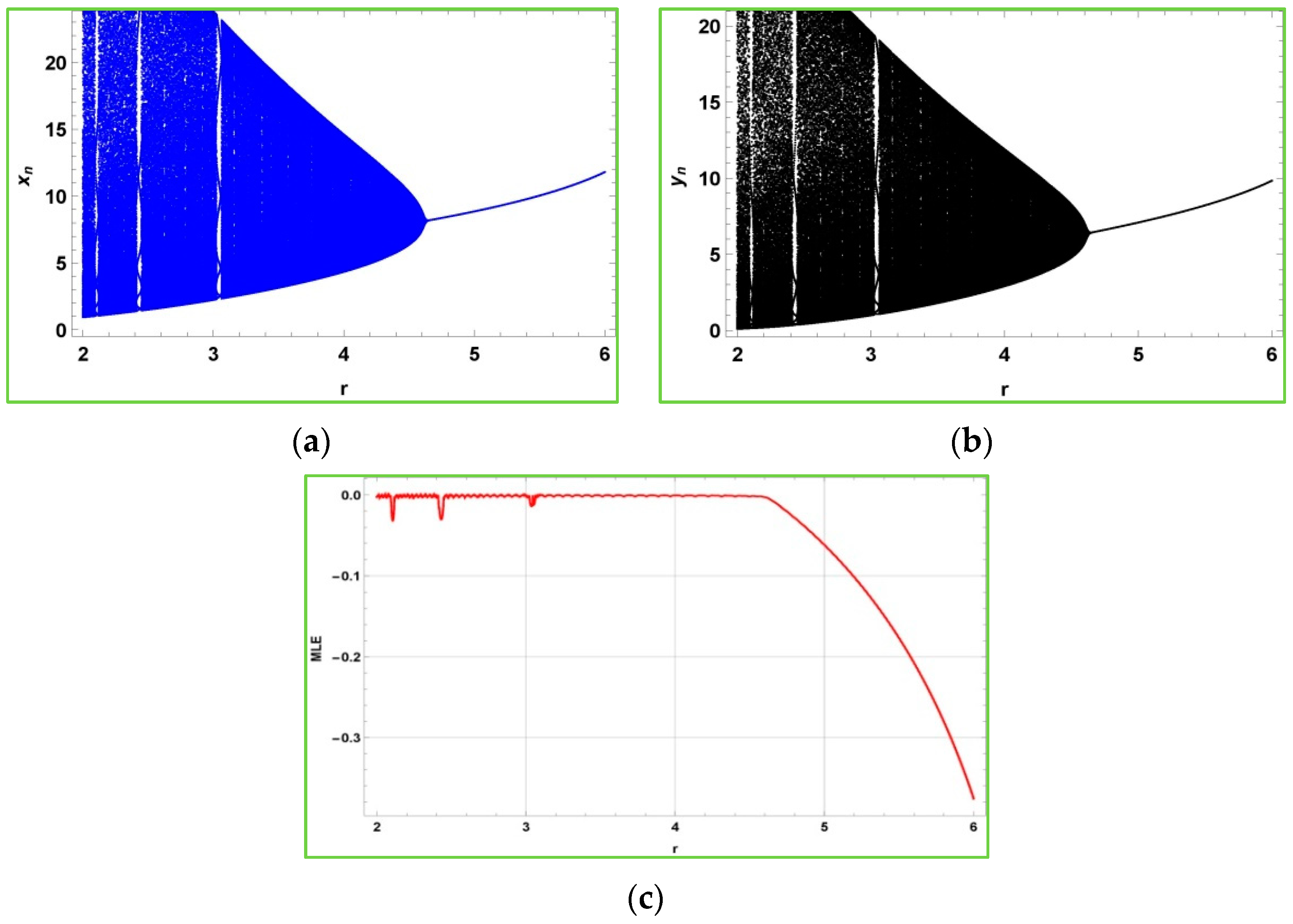
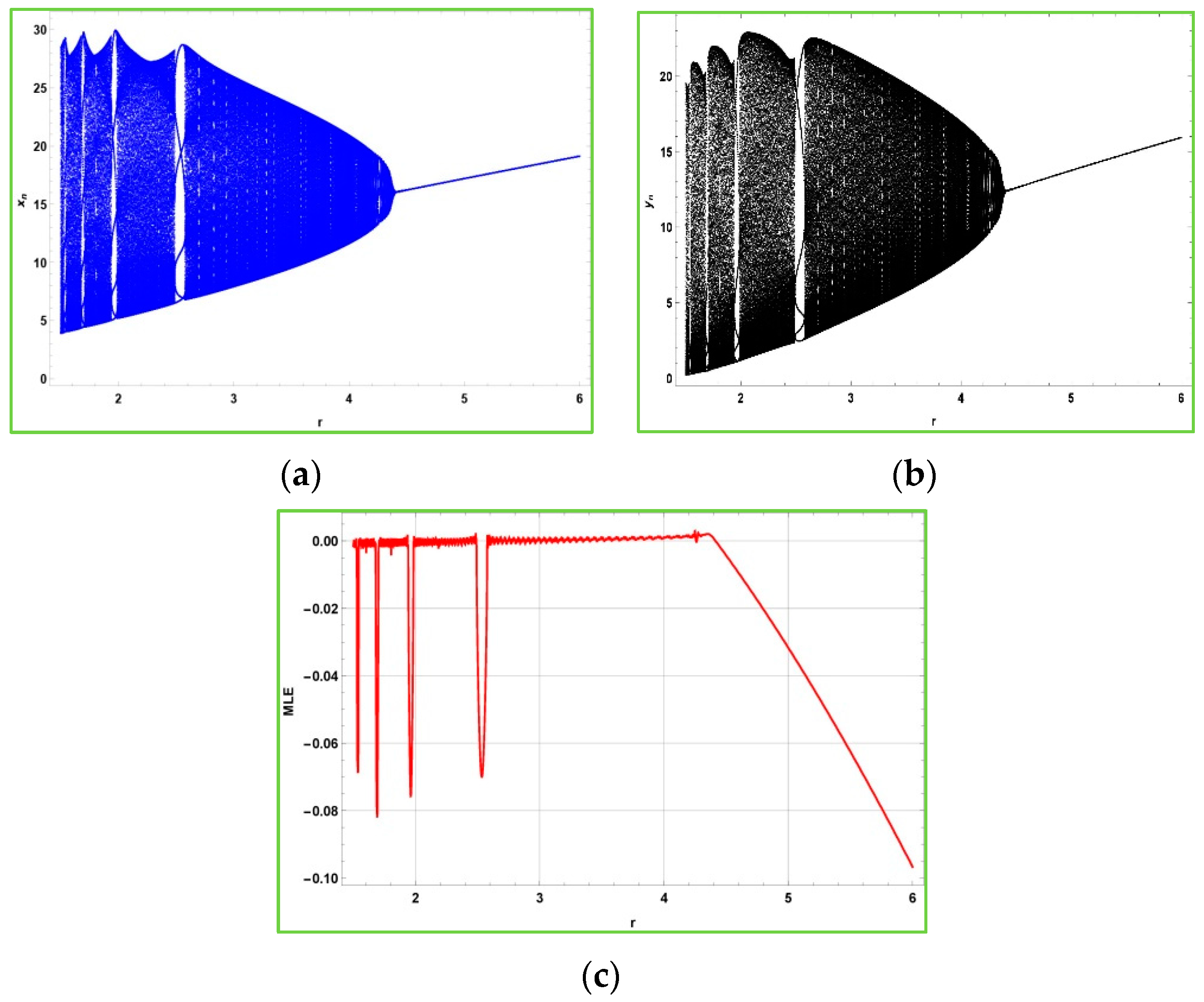
Furthermore, $\left(a,p,r\right)=\left(0.4,0.85, 4.614946371656745\right)$ system (2) has unique positive steady-state which is represented by $\left(x^{*},y^{*}\right)=\left(8.12326, 6.3630567\right)$. For the parametric values $\left(a,p,r\right)=\left(0.4,0.85, 4.614946371656745\right)$ the characteristic polynomial becomes

$$P\left(\lambda \right)={\lambda }^2-1.2166872417286627\lambda +1.$$

Then, the roots of $P\left(\lambda \right)=0$, are ${\lambda }_1=0.608343620864331-0.7936737610338864\mathrm{i}$ and ${\lambda }_1=0.6083436208643314+0.7936737610338864\mathrm{i}$ with $\left|{\lambda }_1\right|=\left|{\lambda }_2\right|=1.$ Therefore, $\left(a,p,r\right)=\left(0.4,0.85, 4.614946371656745\right)\in {\Omega }_{NS}$, then the corresponding bifurcation diagram for model (2) can be shown in the following figures:

Figure 2 shows that after the bifurcation point $r=4.614946371656745$, the populations described in the model (2) experience quasiperiodic behavior due to emergence of Neimark–Sacker bifurcation. Furthermore, $\left(4.614946371656745, 6\right]$ is the non-chaotic region for the model (2), and $\left[2, 4.614946371656745\right]$ is its chaotic region. From Figure 2c, it is obvious to observe that the maximum Lyapunov exponents are almost about zero due to the quasiperiodic behavior.

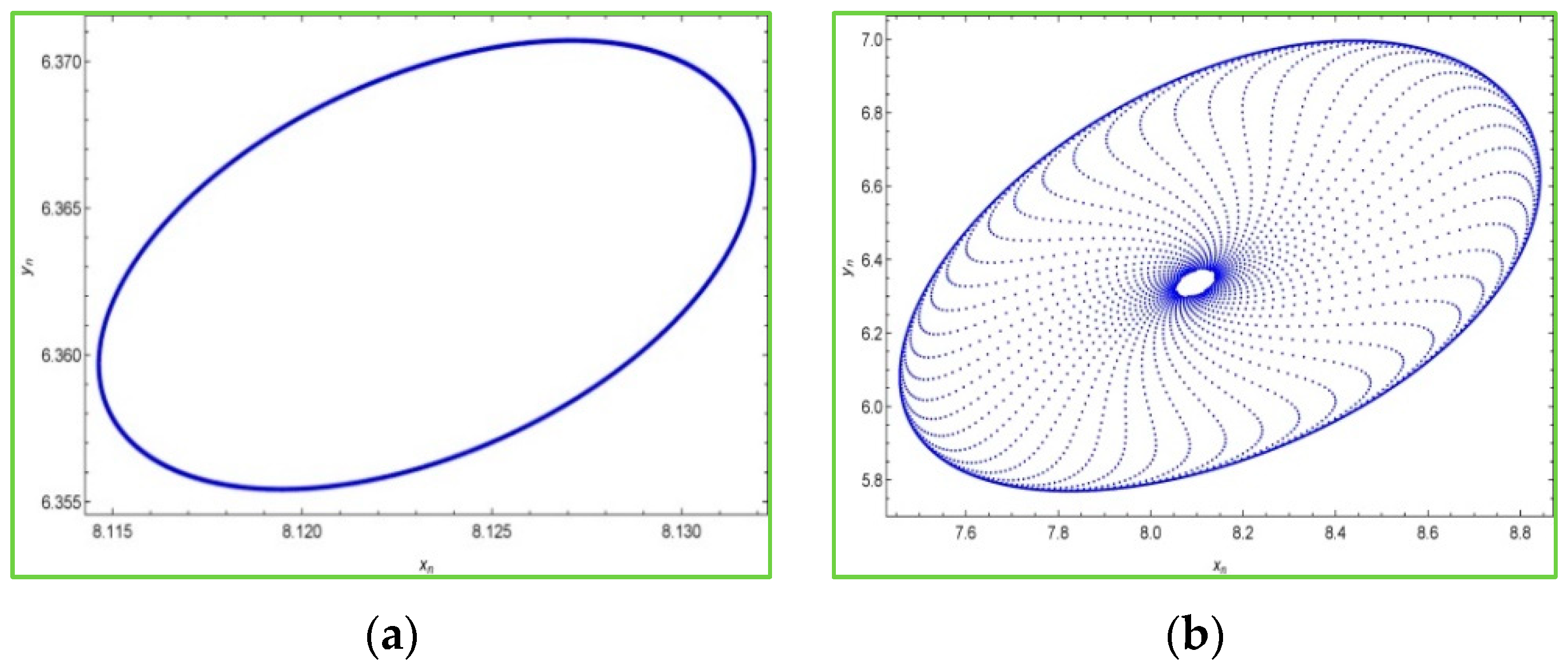
Moreover, it is interesting to see phase portraits of the system (2) for various values of the bifurcation parameter in the chaotic region. For this, we keep fixed $a=0.4$, $p=0.85$ and the initial conditions $\left(x_0,y_0\right)=\left(8.12, 6.36\right)$, and choosing some values of $r$ in the chaotic region, then the phase portraits of the system (2) are portrayed in Figure 3 as follows:

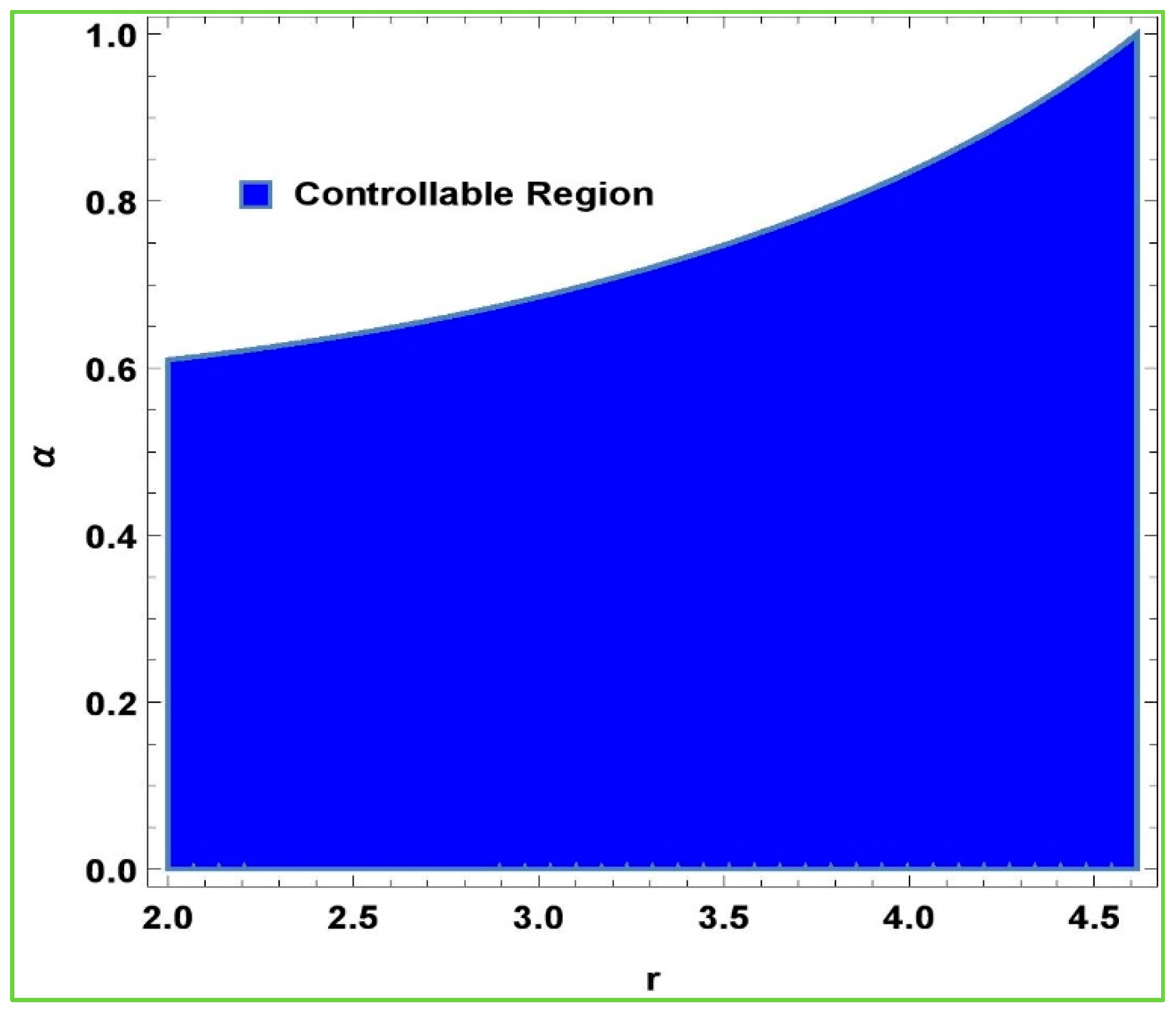
Next, we want to observe the effectiveness of the hybrid control method in the chaotic region due to the emergence of the Hopf bifurcation in the model (2). For this, we choose two fixed parameters, that is, $a=0.4$, $p=0.85$, and keep on varying the other two parameters in the approximate intervals. For this, it is suitable to choose the whole chaotic region $\left[2, 4.614946371656745\right]$ for the bifurcation parameter $r$ and the whole allowable unit interval $\left[0, 1\right]$ for the control parameter $\alpha$. The stability region (controllability region) of system (6) can be shown by Figure 4, which shows the effectiveness of hybrid chaos control methodology:

Example 2.

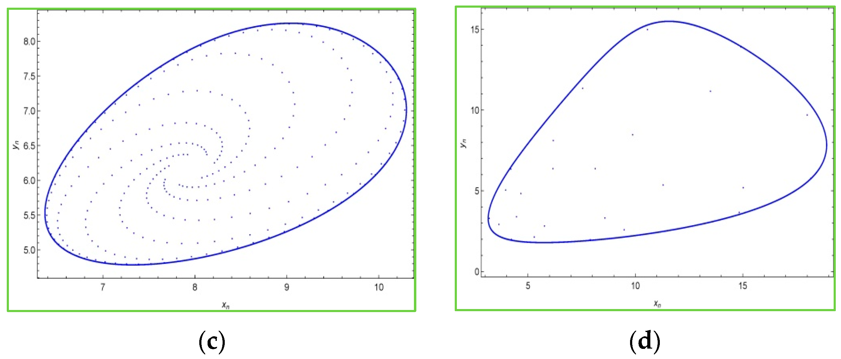
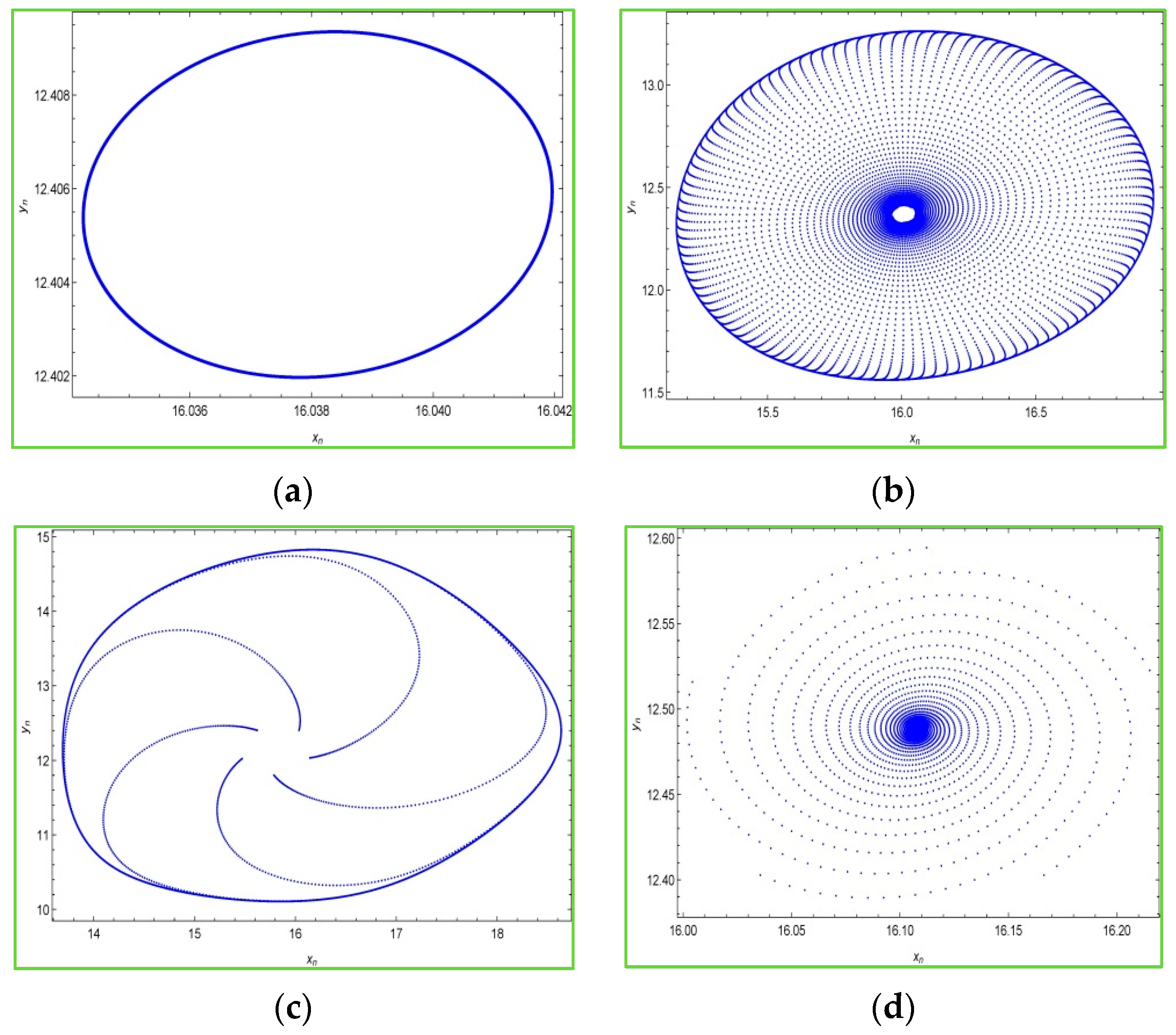
Let $a=0.2$, $H_0=2.5$, $r\in \left[1.5, 6\right]$ and $\left(x_0,y_0\right)=\left(16.035, 12.402\right)$, then system (3) undergoes the Neimark–Sacker bifurcation when $r\approx 4.41524$. The bifurcation diagrams for model (3) can be shown in Figure 5:

The Figure 5 shows that at $r=4.41524$ and $\left(x_0,y_0\right)=\left(16.0356, 12.4027\right),$ model (3) experiences the Neimark–Sacker bifurcation. Furthermore, at $\left(a,H_0,r\right)=\left(0.2, 2.5, 4.41524\right)$ a unique positive equilibrium point exists. The phase portraits of model (3) for $a=0.2$, $H_0=2.5$ and $r\in \left[1.5,6\right]$ are depicted in Figure 6a–d as:

7. Conclusions

The spatial refuge can have important implications for the population dynamics of host–parasitoid systems. The presence of a refuge can increase the survival of the host population, reduce the parasitoid attack rate, lead to increased competition among parasitoids, and make the system more complex and difficult to predict. Therefore, it is important to consider the effects of spatial structure when modeling or studying host–parasitoid systems.

In this manuscript, two host–parasitoid models are discussed. Both the models are modifications of the Nicholson–Bailey model proposed by Bailey et al., in [16]. One of these modifications is to introduce the refuge effect on the classical NB model. For this, we study the two modifications proposed by Hassell. At first, some qualitative features of host–parasitoid models are discussed. These features include the existence of equilibrium points, the stability of equilibria, and the numerical simulations. Moreover, the mathematical results of [2, 3] have been reviewed. They investigated the outcomes of the existence of refuge on the local stability and bifurcation of the models on the three different host–parasitoid models with the spatial refuge effect. The Taylor series method has been used in proposed model (2). It is also proved that model (3) undergoes the Neimark–Sacker bifurcation around the interior equilibrium point. Moreover, it is observed that both proposed models undergo the Neimark–Sacker bifurcation, and the maximum Lyapunov exponents also show that the models experience the Neimark–Sacker bifurcation. In addition to this, the hybrid chaos control methodology is used to control the chaotic behavior of the proposed models. Numerical simulations are provided for further explanation.

References

- Agarwal, T. Bifurcation analysis of a host-parasitoid model with the beddington-deangelis functional response. Glob. J. Math. Anal. 2014, 2, 565–569. [Google Scholar] [CrossRef]
- Bešo, E.; Mujic, N.; Kalabušić, S.; Pilav, E. Neimark–Sacker bifurcation and stability of a certain class of host-parasitoid models with host refuge effect. Int. J. Bifurc. Chaos 2020, 29, 1950169. [Google Scholar] [CrossRef]
- Bešo, E.; Mujic, T.; Kalabušić, S.; Pilav, E. Stability of a certain class of a host-parasitoid model with a spatial refuge effect. J. Biol. Dyn. 2020, 14, 1–31. [Google Scholar] [CrossRef]
- Wu, D.; Zhao, H. Global qualitative analysis of a discrete host-parasitoid model with refuge and strong Allee effects. Math. Methods Appl. Sci. 2018, 41, 2039–2062. [Google Scholar] [CrossRef]
- Din, Q.; Hussain, M. Controlling chaos and Neimark-Sacker bifurcation in a host-parasitoid model. Asian J. Control. 2019, 21, 1202–1215. [Google Scholar] [CrossRef]
- Din, Q.; Saeed, U. Bifurcation analysis and chaos control in a host-parasitoid model. Math. Methods Appl. Sci. 2017, 40, 5391–5406. [Google Scholar] [CrossRef]
- Kapçak, S.; Ufuktepe, U.; Elaydi, S. Stability and invariant manifolds of a generalized Beddington host-parasitoid model. J. Biol. Dyn. 2013, 7, 233–253. [Google Scholar] [CrossRef] [PubMed]
- Livadiotis, G.; Assas, L.; Dennis, B.; Elaydi, S.; Kwessi, E. A discrete-time host–parasitoid model with at Allee effect. J. Biol. Dyn. 2014, 9, 34–51. [Google Scholar] [CrossRef]
- Liu, X.; Chu, Y.; Liu, Y. Bifurcation and chaos in a host-parasitoid model with a lower bound for the host. Adv. Differ. Equ. 2018, 2018, 1–15. [Google Scholar] [CrossRef]
- Ma, X.; Din, Q.; Rafaqat, M.; Javaid, N.; Feng, Y. A Density-dependent host-parasitoid Model with stability, bifurcation and chaos control. Mathematics 2020, 8, 536. [Google Scholar] [CrossRef]
- Schreiber, S.J. Host-parasitoid dynamics of a generalized Thompson model. J. Math. Biol. 2006, 52, 719–732. [Google Scholar] [CrossRef] [PubMed]
- Sebastian, E.; Victor, P. Stability analysis of a host-parasitoid model with logistic growth using Allee effect. Appl. Math. Sci. 2015, 9, 3265–3273. [Google Scholar] [CrossRef]
- Wiggins, S. Introduction to Applied Nonlinear Dynamical Systems and Chaos; Springer: New York, NY, USA, 2003. [Google Scholar]
- Yuan, L.G.; Yang, Q.G. Bifurcation, invariant curve and hybrid control in a discrete-time predator-prey system. Appl. Math. Model. 2015, 39, 2345–2362. [Google Scholar] [CrossRef]
- Luo, X.S.; Chen, G.R.; Wang, B.H.; Fang, J.Q. Hybrid control of period-doubling bifurcation and chaos in discrete nonlinear dynamical systems. Chaos Solitons Fractals 2003, 18, 775–783. [Google Scholar] [CrossRef]
- Bailey, V.A.; Nicholson, J. The balance of animal populations. Proc. Zool. Soc. Lond 1935, 105, 551–598. [Google Scholar] [CrossRef]
- Hassell, M.P. The Dynamics of Arthropod Predator-Prey Systems; Pritnceton Univeristy Press: Princeton, NJ, USA, 1978. [Google Scholar]
- Jury, E.I. Inners and Stability of Dynamic Systems; Research supported by the National Science Foundation; Wiley-Interscience: New York, NY, USA, 1974; Volume 316. [Google Scholar]
- Liu, X.; Xiao, D. Complex dynamic behaviors of a discrete-time predator-prey system. Chaos Solitons Fractals 2007, 32, 80–94. [Google Scholar] [CrossRef]
- Shabbir, M.S.; Din, Q.; Alabdan, R.; Tassaddiq, A.; Ahmad, K. Dynamical complexity in a class of novel discrete-time predator-prey interaction with cannibalism. IEEE Access 2020, 8, 100226–100240. [Google Scholar] [CrossRef]
- Taylor, A.D. Parasitiod competition and the dynamics of host-parasitoid models. Am. Nat. 1988, 132, 417–436. [Google Scholar] [CrossRef]
- Tang, S.Y.; Chen, L.S. Chaos in functional response host-parasitoid ecosystem models. Chaos Solitons Fractals 2002, 13, 875–884. [Google Scholar] [CrossRef]
- Xu, C.L.; Boyce, M.S. Dynamic complexities in a mutual interference host-parasitoid model. Chaos Solitons Fractals 2005, 24, 175–182. [Google Scholar] [CrossRef]
- Jamieson, W.T. On the global behaviour of May’s host-parasitoid model. J. Differ. Equ. Appl. 2019, 25, 583–596. [Google Scholar] [CrossRef]
- Tassaddiq, A.; Shabbir, M.S.; Din, Q. Discretization, bifurcation and control for a class of predator-prey interaction. Fractal Fract. 2022, 6, 31. [Google Scholar] [CrossRef]
- Kaitala, V.; Ylikarjula, J.; Heino, M. Dynamic complexities in host-parasitoid interaction. J. Theor. Biol. 1999, 197, 331–341. [Google Scholar] [CrossRef] [PubMed]