Article

Dynamical Properties of Discrete-Time HTLV-I and HIV-1 within-Host Coinfection Model

by
Ahmed M. Elaiw
*,
Abdulaziz K. Aljahdali
and
Aatef D. Hobiny
Department of Mathematics, Faculty of Science, King Abdulaziz University, Jeddah 21589, Saudi Arabia
*
Author to whom correspondence should be addressed.
Axioms 2023, 12(2), 201; https://doi.org/10.3390/axioms12020201
Submission received: 20 December 2022 / Revised: 30 January 2023 / Accepted: 9 February 2023 / Published: 14 February 2023
(This article belongs to the Special Issue Control Theory and Its Application in Mathematical Biology)

Abstract

:
Infection with human immunodeficiency virus type 1 (HIV-1) or human T-lymphotropic virus type I (HTLV-I) or both can lead to mortality. CD4+T cells are the target for both HTLV-I and HIV-1. In addition, HIV-1 can infect macrophages. CD4+T cells and macrophages play important roles in the immune system response. This article develops and analyzes a discrete-time HTLV-I and HIV-1 co-infection model. The model depicts the within-host interaction of six compartments: uninfected CD4+T cells, HIV-1-infected CD4+T cells, uninfected macrophages, HIV-1-infected macrophages, free HIV-1 particles and HTLV-I-infected CD4+T cells. The discrete-time model is obtained by discretizing the continuous-time model via the nonstandard finite difference (NSFD) approach. We show that NSFD preserves the positivity and boundedness of the model’s solutions. We deduce four threshold parameters that control the existence and stability of the four equilibria of the model. The Lyapunov method is used to examine the global stability of all equilibria. The analytical findings are supported via numerical simulation. The model can be useful when one seeks to design optimal treatment schedules using optimal control theory.

1. Introduction

Mathematical models of within-host viral infection have enhanced our understanding of the dynamical interactions between viruses, target cells and immune cells. The analytical and numerical investigations of these models can be used to (i) estimate the key biological parameters, such as the half-lives of the virus and infected cell, and the daily viral production; (ii) estimate different antiviral drug efficacies; (iii) evaluate the intensity of the immune system responses; (iv) predict disease progression over long terms [1]. Many scientists and researchers were interested in formulating and studying mathematical models of the within-host dynamics of different viruses that attack humans, such as human immunodeficiency virus type 1 (HIV-1) [2,3,4,5,6,7,8,9,10,11,12,13,14], human T-lymphotropic virus type I (HTLV-I) [15,16,17,18,19,20], hepatitis B virus (HBV) [21], hepatitis C virus (HCV), [22], influenza [23], dengue virus [24], Chikungunya virus [25], ebola virus [26] and recently severe acute respiratory syndrome coronavirus 2 (SARS-CoV-2) [27,28,29].
HIV-1 is a retrovirus that attacks the fundamental component of the immune system, CD 4 + T cells. Infection with this virus causes a breakdown in the immune system, exposing the human body to opportunistic diseases. The disease caused by HIV-1 is the acquired immunodeficiency syndrome (AIDS). The two main immune responses against the viral infection are cytotoxic T lymphocyte (CTL) immune response and antibody immune response. CTLs attack and kill the viral infected cells. Antibodies produced by B cells are responsible for neutralizing viruses. The basic HIV-1 dynamics model presented in [2] includes three compartments: uninfected CD4 + T cells (x), HIV-1-infected CD4 + T cells (y) and free HIV-1 particles (v) as:
d x d t = ξ CD 4 + T cells production γ x death ω x v HIV - 1 infectious transmission ,
d y d t = ω x v HIV - 1 infectious transmission α y death ,
d v d t = β α y generation of HIV - 1 θ v death .
Many mathematical models were formulated as an extension of the basic HIV-1 model (1)–(3) to take into account many biological factors such as time delay [5,6], drug therapies [6,7], CTL immunity [2], antibody immunity [8], reaction-diffusion [9], stochastic effects [10] and latent HIV-1 reservoirs [4].
It was found in [4] that HIV-1 can infect macrophages in addition to CD4 + T cells. Mathematical HIV-1 models that include macrophages as a second target for HIV-1 are more reasonable and accurate. The HIV-1 infection model with two categories of target cells was presented in [7,11] as:
d x d t = ξ 1 CD 4 + T cells production γ 1 x death ω 1 x v HIV - 1 infectious transmission , d y d t = ω 1 x v HIV - 1 infectious transmission α 1 y death , d w d t = ξ 2 macrophages production γ 2 w death ω 2 w v HIV - 1 infectious transmission , d z d t = ω 2 w v HIV - 1 infectious transmission α 2 z death , d v d t = β 1 α 1 y + β 2 α 2 z generation of HIV - 1 θ v death ,
where w and z are the concentrations of uninfected macrophages and HIV-1-infected macrophages, respectively. This model was extended in several directions by including optimal treatment schedules [12,13], CTL immunity [14], antibody immunity [30], time delay [30], latent infection [3] and stochastic effects [14].
HTLV-I is a retrovirus that infects the CD 4 + T cells. HTLV-I-associated myelopathy/tropical spastic paraparesis (HAM/TSP) and adult T-cell leukemia (ATL) diseases are the cause of HTLV-I infection. A mathematical HTLV-I infection model without considering the CTL is given as [16]:
d x d t = ξ 1 CD 4 + T cells production γ 1 x death ω 3 x u HTLV - I infectious transmission , d u d t = ω 3 x u HTLV - I infectious transmission δ u death ,
where u represents the concentration of HTLV-I-infected CD4 + T cells.
HTLV-I infection models with CTL immune response were addressed in [15,16,17,18]. HTLV-I infection models have been incorporated with intracellular delay in [19,20], and with immune response delay in [18,19]. Reaction–diffusion HTLV-I infection models were investigated in [17].
Both HTLV-I and HIV-1 can be transmitted from an infected individual to healthy individuals through blood transfusions, sexual relationships, organ transplantation and infected sharp objects. HTLV-I and HIV-1 co-infection models were developed and analyzed in [31,32]. In these papers, the presence of macrophages in the HIV-1 dynamics as a second target was not considered. This shortcoming was addressed by modeling the HTLV-I and HIV-1 co-infection as follows [33]:
d x d t = ξ 1 CD 4 + T cells production γ 1 x death ω 1 x v HIV - 1 infectious transmission ω 3 x u HTLV - I infectious transmission ,
d y d t = ω 1 x v HIV - 1 infectious transmission α 1 y death ,
d w d t = ξ 2 macrophages production γ 2 w death ω 2 w v HIV - 1 infectious transmission ,
d z d t = ω 2 w v HIV - 1 infectious transmission α 2 z death ,
d v d t = β 1 α 1 y + β 2 α 2 z generation of HIV - 1 θ v death ,
d u d t = ω 3 x u HTLV - I infectious transmission δ u death .
The analytical solutions for the above-mentioned continuous-time models are unknown due to their nonlinearity. Therefore, numerical discretization is usually used to solve such models. In addition, the real measurements from viral infected individuals are usually taken at discrete-time instants. For these reasons, studying the resulting discrete-time models is important. One important question arises: how can we choose a suitable discretization scheme such that the basic and global properties of solutions of the corresponding continuous-time models can be efficiently maintained? Standard numerical methods for solving nonlinear differential equations such as Euler, Runge–Kutta and others suffer from numerical instability and bias when large step sizes are used in the numerical simulation [34]. In this case, these methods can give non-physical solutions and can produce “false” or “spurious” fixed points, which are not fixed points of the original continuous-time model [35,36]. Based on carefully designed rules, Mickens [37,38] introduced a non-standard finite difference (NSFD) scheme, which has been successfully used in the study of different biological models in epidemiology [35,36,39] and virology [40,41,42]. These models are described by different types of differential equations: ordinary differential equations (ODEs), partial differential equations (PDEs) and fractional differential equations (FDEs). The main advantage of the NSFD method is that the essential qualitative features of the mathematical model such as equilibria, positivity (or nonnegativity), boundedness and global behaviors of solutions are preserved independently of the selected step-size [40]. The NSFD method was applied to discretize continuous-time HIV-1 infection models within a host in [43,44,45,46,47]. In [44], a discrete-time HIV-1 model with the cure rate and Beddington–DeAngelis incidence was studied. Local stability of equilibria was established. Elaiw and Alshaikh [47] studied the global stability of two discrete-time HIV-1 models by including three types of HIV-1-infected cells: latently, long-lived chronically and short-lived. Liu and Zhu [45] developed an HIV-1 infection model with CTL immunity, time delay and diffusion. The system was given by PDEs, and it was discretized via the NSFD method. The global stability of the model’s equilibria was proven via the Lyapunov method.
We noted that the discrete-time version of the within-host HTLV-I single-infection model and the HTLV-I/HIV-1 co-infection model were not studied before. The aim of the present article is to discretize the HIV-1 and HTLV-I co-infection model (4)–(9) using the NSFD method. We first establish the positivity and ultimate boundedness of the discrete-time model’s solutions and then calculate all equilibria and deduce their existence conditions. We examine the global stability of the four equilibria using the Lyapunov approach. We present some numerical simulations to clarify the theoretical results.

2. Discrete-Time HTLV-I and HIV-1 Co-Infection Model

Applying the NSFD approach to system (4)–(9), we get
x n + 1 x n Ω ( h ) = ξ 1 γ 1 x n + 1 ω 1 x n + 1 v n ω 3 x n + 1 u n ,
y n + 1 y n Ω ( h ) = ω 1 x n + 1 v n α 1 y n + 1 ,
w n + 1 w n Ω ( h ) = ξ 2 γ 2 w n + 1 ω 2 w n + 1 v n ,
z n + 1 z n Ω ( h ) = ω 2 w n + 1 v n α 2 z n + 1 ,
v n + 1 v n Ω ( h ) = β 1 α 1 y n + 1 + β 2 α 2 z n + 1 θ v n + 1 ,
u n + 1 u n Ω ( h ) = ω 3 x n + 1 u n δ u n + 1 ,
where h > 0 is the time step and ( x n , , y n , w n , z n , v n , u n ) are the approximations of the solution ( x ( t n ) , y ( t n ) , w ( t n ) , z ( t n ) , v ( t n ) , u ( t n ) ) of the system (4)–(9) at the discrete time point t n = n h , n N = { 0 , 1 , 2 , } . The denominator function Ω ( h ) is selected such that Ω ( h ) = h + O ( h 2 ) . We consider the following form of Ω ( h ) [48]:
Ω ( h ) = 1 e γ 1 h γ 1 .
The initial conditions of system (10)–(15) are
( x 0 , y 0 , w 0 , z 0 , v 0 , u 0 ) R + 6 = { ( x , y , w , z , v , u ) x > 0 , y > 0 , w > 0 , z > 0 , v > 0 , u > 0 } .
The discrete-time HTLV-I and HIV-1 co-infection model (10)–(15) may be useful to develop several viral co-infection models such as SARS-CoV-2 and co-infection with other respiratory viruses.

3. Preliminaries

Let σ = min { γ 1 , α 1 , δ , γ 2 , α 2 } and ξ 12 = ξ 1 + ξ 2 and define the sets
Γ = ( x , y , w , z , u , v ) R + 6 : x ξ 1 γ 1 , w ξ 2 γ 2 , x + y + w + z + u ξ 12 σ , v ( β 1 α 1 + β 2 α 2 ) ξ 12 θ σ , Υ = ( x , 0 , w , 0 , 0 , 0 ) R + 6 : x 0 , w 0 .
Lemma 1.
Any solution ( x , y , w , z , v , u ) of models (10)–(15) with initial conditions (17) is positive and ultimately bounded.
Proof. 
Equations (10)–(15) imply that
x n + 1 = Ω ( h ) ξ 1 + x n 1 + Ω ( h ) ( γ 1 + ω 1 v n + ω 3 u n ) ,
y n + 1 = Ω ( h ) ω 1 x n + 1 v n + y n 1 + Ω ( h ) α 1 ,
w n + 1 = Ω ( h ) ξ 2 + w n 1 + Ω ( h ) ( γ 2 + ω 2 v n ) ,
z n + 1 = Ω ( h ) ω 2 w n + 1 v n + z n 1 + Ω ( h ) α 2 , v n + 1 = Ω ( h ) ( β 1 α 1 y n + 1 + β 2 α 2 z n + 1 ) + v n 1 + Ω ( h ) θ ,
u n + 1 = u n + Ω ( h ) ω 3 x n + 1 u n 1 + Ω ( h ) δ .
Since all parameters of models (4)–(9) are positive and the initial values are also positive, then by induction we obtain x n > 0 , y n > 0 , w n > 0 , z n > 0 , v n > 0 and u n > 0 for all n N .
From Equations (10) and (12), we have
x n + 1 x n Ω ( h ) ξ 1 γ 1 x n + 1 x n + 1 x n 1 + γ 1 Ω ( h ) + ξ 1 Ω ( h ) 1 + γ 1 Ω ( h ) w n + 1 w n Ω ( h ) ξ 2 γ 2 w n + 1 w n + 1 w n 1 + γ 2 Ω ( h ) + ξ 2 Ω ( h ) 1 + γ 2 Ω ( h ) .
By Lemma 2.2 in [49] we get
x n 1 1 + Ω ( h ) γ 1 n x 0 + ξ 1 γ 1 1 1 1 + Ω ( h ) γ 1 n , w n 1 1 + Ω ( h ) γ 2 n w 0 + ξ 2 γ 2 1 1 1 + Ω ( h ) γ 2 n .
Consequently, lim sup n x n ξ 1 γ 1 and lim sup n w n ξ 2 γ 2 . We define the following sequence M n :
M n = x n + y n + w n + z n + u n .
Hence
M n + 1 M n = ( x n + 1 x n ) + ( y n + 1 y n ) + ( w n + 1 w n ) + ( z n + 1 z n ) + ( u n + 1 u n ) = Ω ( h ) ξ 1 γ 1 x n + 1 ω 1 x n + 1 v n ω 3 x n + 1 u n + ω 1 x n + 1 v n + α 1 y n + 1 + ξ 2 γ 2 w n + 1 ω 2 w n + 1 v n + ω 2 w n + 1 v n α 2 z n + 1 + ω 3 x n + 1 u n δ u n + 1 = Ω ( h ) ξ 1 γ 1 x n + 1 α 1 y n + 1 + ξ 2 γ 2 w n + 1 α 2 z n + 1 δ u n + 1 Ω ( h ) ξ 12 Ω ( h ) σ [ x n + 1 + y n + 1 + w n + 1 + z n + 1 + u n + 1 ] = Ω ( h ) ξ 12 Ω ( h ) σ M n + 1 ,
and
M n + 1 M n 1 + Ω ( h ) σ + Ω ( h ) ξ 12 1 + Ω ( h ) σ .
It follows that
M n 1 1 + Ω ( h ) σ n M 0 + ξ 12 σ 1 1 1 + Ω ( h ) σ n .
Consequently, lim sup n M n ξ 12 σ . We have
v n + 1 v n = Ω ( h ) β 1 α 1 y n + 1 + β 2 α 2 z n + 1 θ v n + 1 Ω ( h ) β 1 α 1 ξ 12 σ + β 2 α 2 ξ 12 σ θ v n + 1 .
Hence,
v n + 1 v n 1 + Ω ( h ) θ + Ω ( h ) ( β 1 α 1 + β 2 α 2 ) ξ 12 ( 1 + Ω ( h ) θ ) σ .
By induction, we get
v n 1 1 + Ω ( h ) θ n v 0 + ( β 1 α 1 + β 2 α 2 ) ξ 12 θ σ 1 1 1 + Ω ( h ) θ n .
Consequently, lim sup n v n ( β 1 α 1 + β 2 α 2 ) ξ 12 θ σ . Therefore ( x n , y n , w n , z n , v n , u n ) converge to Γ as n .

4. Equilibria

Here, we calculate the model’s equilibria and deduce their existence conditions.
Lemma 2.
Models (10)–(15) have four equilibria determined by four threshold parameters R j > 0 , j = 0 , 1 , 2 , 3 :
(1) Infection-free equilibrium E Q 0 = ( x 0 , 0 , w 0 , 0 , 0 , 0 ) , which always exists.
(2) Chronic HIV-1 single-infection equilibrium E Q 1 = ( x ^ , y ^ , w ^ , z ^ , v ^ , 0 ) exists when R 0 = R 01 + R 02 > 1 .
(3) Chronic HTLV-I single-infection equilibrium E Q 2 = ( x ˜ , 0 , w ˜ , 0 , 0 , u ˜ ) exists when R 1 > 1 .
(4) Chronic HTLV-I/HIV-1 co-infection equilibrium E Q 3 = ( x ¯ , y ¯ , w ¯ , z ¯ , v ¯ , u ¯ ) exists when R 1 R 01 > 1 ,   R 2 > 1 and R 3 > 1 .
Proof. 
Any equilibrium E Q = ( x , y , w , z , v , u ) satisfies
0 = ξ 1 γ 1 x ω 1 x v ω 3 x u ,
0 = ω 1 x v α 1 y ,
0 = ξ 2 γ 2 w ω 2 w v ,
0 = ω 2 w v α 2 z ,
0 = β 1 α 1 y + β 2 α 2 w θ v ,
0 = ω 3 x u δ u .
From Equation (28), we get two options: u = 0 and x = δ ω 3 . First, we consider u = 0 ; then, from Equations (24) and (26), we get
y = ω 1 x v α 1 and z = ω 2 w v α 2 .
Now, substituting in Equation (27), we get
( β 1 ω 1 x + β 2 ω 2 w θ ) v = 0 .
There are two solutions to Equation (30): v = 0 and β 1 α 1 x + β 2 α 2 w θ . When v = 0 , we get y = 0 and z = 0 , which gives infection-free equilibrium E Q 0 = ( x 0 , 0 , w 0 , 0 , 0 , 0 ) , where
x 0 = ξ 1 γ 1 and w 0 = ξ 2 γ 2 .
When v 0 and β 1 ω 1 x + β 2 ω 2 w θ = 0 , then from Equations (23) and (25), we get
β 1 ω 1 ξ 1 γ 1 + ω 1 v + β 2 ω 2 ξ 2 γ 2 + ω 2 v θ = 0 .
We define a function H as
H ( v ) = β 1 ω 1 ξ 1 γ 1 + ω 1 v + β 2 ω 2 ξ 2 γ 2 + ω 2 v θ = 0 .
Then,
H ( 0 ) = β 1 ω 1 ξ 1 γ 1 + β 2 ω 2 ξ 2 γ 2 θ = θ β 1 ω 1 ξ 1 γ 1 θ + β 2 ω 2 ξ 2 γ 2 θ 1 = θ ( R 0 1 ) ,
where
R 0 = R 01 + R 02 , R 01 = β 1 ω 1 ξ 1 γ 1 θ and R 02 = β 2 ω 2 ξ 2 γ 2 θ .
Thus H ( 0 ) > 0 , when R 0 > 1 . The parameter R 0 represents the basic HIV-1 single-infection reproductive number.
lim v H ( v ) = θ .
Further,
H ( v ) = β 1 ξ 1 ω 1 2 ( γ 1 + ω 1 v ) 2 + β 2 ξ 2 ω 2 2 ( γ 2 + ω 2 v ) 2 < 0 .
Hence, H is a strictly decreasing function of v, and thus there exists a unique v ^ ( 0 , ) such that H ( v ^ ) = 0 . It follows that
x ^ = ξ 1 γ 1 + ω 1 v ^ > 0 and w ^ = ξ 2 γ 2 + ω 2 v ^ > 0 .
Then, Equation (29) gives
y ^ = ω 1 x ^ v ^ α 1 > 0 and z ^ = ω 2 w ^ v ^ α 2 > 0 .
Here, v ^ satisfies the following quadratic equation:
A v ^ 2 + B v ^ + C = 0 ,
with
A = θ ω 1 ω 2 ,
B = θ γ 1 ω 2 + θ γ 2 ω 1 ω 1 ω 2 ( β 1 ξ 1 + β 2 ξ 2 ) ,
C = θ γ 1 γ 2 β 1 γ 2 ω 1 ξ 1 β 2 γ 1 ω 2 ξ 2 = θ γ 1 γ 2 1 β 1 ω 1 ξ 1 γ 1 θ β 2 ω 2 ξ 2 γ 2 θ = θ γ 1 γ 2 ( R 0 1 ) .
Obviously, C < 0 when R 0 > 1 . Equation (31) has a positive root as
v ^ = B + B 2 4 A C 2 A > 0 .
Hence, the chronic HIV-1 single-infection equilibrium E Q 1 = ( x ^ , y ^ , w ^ , z ^ , v ^ , 0 ) exists when R 0 > 1 .
Now consider x ˜ = δ ω 3 and u 0 . Solving Equations (23)–(27), we obtain two equilibria: the chronic HTLV-I single-infection equilibrium E Q 2 = ( x ˜ , 0 . w ˜ , 0 , 0 , u ˜ ) , where
x ˜ = δ ω 3 , w ˜ = ξ 2 γ 2 = w 0 , u ˜ = γ 1 ω 3 ( R 1 1 ) ,
where
R 1 = ω 3 ξ 1 γ 2 δ .
Parameter R 1 is the basic HTLV-I single-infection reproductive number. Consequently, E Q 2 exists when R 1 > 1 . The other equilibrium is the chronic HTLV-I/HIV-1 co-infection equilibrium E Q 3 = ( x ¯ , y ¯ , w ¯ , z ¯ , v ¯ , u ¯ ) , where
x ¯ = δ ω 3 = x ˜ , y ¯ = γ 2 ω 1 δ α 1 ω 2 ω 3 ( R 2 1 ) , v ¯ = γ 2 ω 2 ( R 2 1 ) , w ¯ = w 0 R 2 , z ¯ = w 0 R 2 ( R 2 1 ) = ξ 2 α 2 R 02 R 02 + R 01 R 1 1 , u ¯ = γ 2 ω 1 ω 2 ω 3 ( R 2 1 ) ( R 3 1 ) ,
and
R 2 = ξ 2 β 2 ω 2 ω 3 γ 2 β 1 ω 1 δ R 1 R 01 1 , R 3 = γ 1 ω 2 γ 2 ω 1 R 1 1 R 2 1 .
We can see that, E Q 3 exists when R 1 R 01 > 1 , R 2 > 1 and R 3 > 1 . □

5. Global Stability

In this section, we demonstrate the global asymptotic stability of all equilibria by establishing appropriate Lyapunov functions. Define a function G ( x ) 0 as G ( x ) = x 1 ln x . We have
ln x x 1 .
Theorem 1.
If R 0 1 and R 1 1 , then E Q 0 = ( x 0 , 0 , w 0 , 0 , 0 , 0 ) is globally asymptotically stable (GAS) in Γ.
Proof. 
Define a discrete Lyapunov function Λ n ( x n , y n , w n , z n , v n , u n ) as
Λ n = 1 Ω ( h ) x 0 G x n x 0 + y n + β 2 w 0 β 1 G w n w 0 + β 2 β 1 z n + 1 β 1 ( 1 + Ω ( h ) θ ) v n + ( 1 + Ω ( h ) δ ) u n .
Clearly, Λ n > 0 for all x n > 0 , y n > 0 , w n > 0 , z n > 0 , v n > 0 , u n > 0 . In addition, Λ n ( x 0 , 0 , w 0 , 0 , 0 , 0 ) = 0 . Evaluating the difference Δ Λ n = Λ n + 1 Λ n as
Δ Λ n = Λ n + 1 Λ n = 1 Ω ( h ) x 0 G x n + 1 x 0 + y n + 1 + β 2 w 0 β 1 G w n + 1 w 0 + β 2 β 1 z n + 1 + 1 β 1 ( 1 + Ω ( h ) θ ) v n + 1 + ( 1 + Ω ( h ) δ ) u n + 1 x 0 G x n x 0 y n β 2 w 0 β 1 G w n w 0 β 2 β 1 z n 1 β 1 ( 1 + Ω ( h ) θ ) v n ( 1 + Ω ( h ) δ ) u n = 1 Ω ( h ) x 0 x n + 1 x n x 0 + ln x n x n + 1 + y n + 1 y n + β 2 w 0 β 1 w n + 1 w n w 0 + ln w n w n + 1 + β 2 β 1 z n + 1 z n + 1 β 1 ( 1 + Ω ( h ) θ ) v n + 1 v n + ( 1 + Ω ( h ) δ ) u n + 1 u n .
Using inequality (33), we obtain
Δ Λ n 1 Ω ( h ) x n + 1 x n + x 0 x n x n + 1 1 + y n + 1 y n + β 2 β 1 w n + 1 w n + w 0 w n w n + 1 1 + β 2 β 1 z n + 1 z n + 1 β 1 ( 1 + Ω ( h ) θ ) v n + 1 v n + ( 1 + Ω ( h ) δ ) u n + 1 u n = 1 Ω ( h ) 1 x 0 x n + 1 x n + 1 x n + y n + 1 y n + β 2 β 1 1 w 0 w n + 1 w n + 1 w n + β 2 β 1 z n + 1 z n + 1 β 1 ( 1 + Ω ( h ) θ ) v n + 1 v n + ( 1 + Ω ( h ) δ ) u n + 1 u n .
From Equations (10)–(15), we have
Δ Λ n 1 x 0 x n + 1 ξ 1 γ 1 x n + 1 ω 1 x n + 1 v n ω 3 x n + 1 u n + ω 1 x n + 1 v n α 1 y n + 1 + β 2 β 1 1 w 0 w n + 1 ξ 2 γ 2 w n + 1 ω 2 w n + 1 v n + β 2 β 1 ω 2 w n + 1 v n α 2 z n + 1 + 1 β 1 β 1 α 1 y n + 1 + β 2 α 2 z n + 1 θ v n + 1 + θ β 1 v n + 1 v n + ω 3 x n + 1 u n δ u n + 1 + δ u n + 1 u n = 1 x 0 x n + 1 ξ 1 γ 1 x n + 1 + β 2 β 1 1 w 0 w n + 1 ( ξ 2 γ 2 w n + 1 ) + β 2 β 1 ω 2 w 0 + ω 1 x 0 θ β 1 v n + ( ω 3 x 0 δ ) u n .
We have
ξ 1 = γ 1 x 0 , ξ 2 = γ 2 w 0 ,
then, we obtain
Δ Λ n 1 x 0 x n + 1 ( γ 1 x 0 γ 1 x n + 1 ) + β 2 β 1 1 w 0 w n + 1 ( γ 2 w 0 γ 2 w n + 1 ) + β 2 β 1 ω 2 w 0 + ω 1 x 0 θ β 1 v n + ( ω 3 x 0 δ ) u n = γ 1 x n + 1 x 0 2 x n + 1 γ 2 β 2 β 1 ( w n + 1 w 0 ) 2 w n + 1 + θ β 1 ω 1 β 1 ξ 1 θ γ 1 + ω 2 β 2 ξ 2 θ γ 2 1 v n + δ ω 3 ξ 1 δ γ 1 1 u n = γ 1 x n + 1 x 0 2 x n + 1 γ 2 β 2 β 1 ( w n + 1 w 0 ) 2 w n + 1 + θ β 1 ( R 0 1 ) v n + δ ( R 1 1 ) u n .
Since R 0 1 and R 1 1 , then Λ n is monotonically decreasing. Clearly, Λ n 0 , and hence there is a limit lim n Λ n 0 , and thus lim n Δ Λ n = 0 , which gives lim n x n = x 0 , lim n w n = w 0 , lim n ( R 0 1 ) v n = 0 and lim n ( R 1 1 ) u n = 0 . We consider four cases:
(i) R 0 = 1 and R 1 = 1 , and then from Equation (12),
0 = ξ 2 γ 2 w 0 ω 2 w 0 lim n v n lim n v n = 0 .
In addition, from Equations (10) and (14),
0 = ξ 1 γ 1 x 0 ω 1 x 0 lim n v n ω 3 x 0 lim n u n lim n u n = 0 ,
0 = β 1 α 1 lim n y n + 1 + β 2 α 2 lim n z n + 1 θ lim n v n + 1 lim n y n = lim n z n = 0
(ii) R 0 = 1 , R 1 < 1 and lim n u n = 0 . Equations (34) and (36) yield lim n v n = lim n y n = lim n z n = 0 .
(iii) R 0 < 1 , R 1 = 1 and lim n v n = 0 . Equations (35) and (36) give lim n u n = lim n y n = lim n z n = 0 .
(iv) R 0 < 1 , R 1 < 1 and lim n v n = lim n u n = 0 . From Equation (36), we get lim n y n = lim n z n = 0 .
Consequently, if R 0 1 and R 1 1 , then lim n x n = x 0 , lim n w n = w 0 and lim n y n = lim n z n = lim n v n = lim n u n = 0 . This shows that E Q 0 is GAS. □
The result of Theorem 1 shows that if there exist control parameters (e.g., drug therapies) that make R 0 1 and R 1 1 , then both HTLV-I and HIV-1 will be removed from the body regardless of the initial states.
Theorem 2.
If R 0 > 1 and R 1 1 , then E Q 1 GAS in Γ \ Υ .
Proof. 
Define
Θ n = 1 Ω ( h ) x ^ G x n x ^ + y ^ G y n y ^ + β 2 w ^ β 1 G w n w ^ + β 2 z ^ β 1 G z n z ^ + v ^ β 1 ( 1 + Ω ( h ) θ ) G v n v ^ + ( 1 + Ω ( h ) δ ) u n .
Clearly Θ n > 0 for all x n > 0 , y n > 0 , w n > 0 , z n > 0 ,   v n > 0 and u n > 0 . In addition Θ n ( x ^ , y ^ , w ^ , z ^ , v ^ , 0 ) = 0 . Computing the difference Δ Θ n = Θ n + 1 Θ n as:
Δ Θ n = 1 Ω ( h ) x ^ G x n + 1 x ^ + y ^ G y n + 1 y ^ + β 2 w ^ β 1 G w n + 1 w ^ + β 2 z ^ β 1 G z n + 1 z ^ + v ^ β 1 ( 1 + Ω ( h ) θ ) G v n + 1 v ^ + ( 1 + Ω ( h ) δ ) u n + 1 x ^ G x n x ^ y ^ G y n y ^ β 2 w ^ β 1 G w n w ^ β 2 z ^ β 1 G z n z ^ v ^ β 1 ( 1 + Ω ( h ) θ ) G v n v ^ ( 1 + Ω ( h ) δ ) u n = 1 Ω ( h ) x ^ x n + 1 x ^ x n x ^ + ln x n x n + 1 + y ^ y n + 1 y ^ y n y ^ + ln y n y n + 1 + β 2 β 1 w ^ w n + 1 w ^ w n w ^ + ln w n w n + 1 + β 2 β 1 z ^ z n + 1 z ^ z n z ^ + ln z n z n + 1 + 1 β 1 ( 1 + Ω ( h ) θ ) v ^ v n + 1 v ^ v n v ^ + ln v n v n + 1 + ( 1 + Ω ( h ) δ ) u n + 1 u n .
Using inequality (33), we have
Δ Θ n 1 Ω ( h ) x n + 1 x n + x ^ x n x n + 1 1 + y n + 1 y n + y ^ y n y n + 1 1 + β 2 β 1 w n + 1 w n + w ^ w n w n + 1 1 + β 2 β 1 z n + 1 z n + z ^ z n z n + 1 1 + 1 β 1 v n + 1 v n + v ^ v n v n + 1 1 + ( 1 + Ω ( h ) δ ) u n + 1 u n + θ β 1 v n + 1 v n + v ^ ln v n v n + 1 = 1 Ω ( h ) 1 x ^ x n + 1 x n + 1 x n + 1 y ^ y n + 1 y n + 1 y n + β 2 β 1 1 w ^ w n + 1 w n + 1 w n + β 2 β 1 1 z ^ z n + 1 z n + 1 z n + 1 β 1 1 v ^ v n + 1 v n + 1 v n + ( 1 + Ω ( h ) δ ) u n + 1 u n + θ v n + 1 β 1 θ β 1 v n + θ v ^ β 1 ln v n v n + 1 .
From Equations (10)–(15), we have
Δ Θ n 1 x ^ x n + 1 ( ξ 1 γ 1 x n + 1 ω 1 x n + 1 v n ω 3 x n + 1 u n ) + 1 y ^ y n + 1 ( ω 1 x n + 1 v n α 1 y n + 1 ) + β 2 β 1 1 w ^ w n + 1 ( ξ 2 γ 2 w n + 1 ω 2 w n + 1 v n ) + β 2 β 1 1 z ^ z n + 1 ( ω 2 w n + 1 v n α 2 z n + 1 ) + 1 β 1 1 v ^ v n + 1 ( β 1 α 1 y n + 1 + β 2 α 2 z n + 1 θ v n + 1 ) + θ v n + 1 β 1 θ v n β 1 + θ β 1 v ^ ln v n v n + 1 + ( ω 3 x n + 1 u n δ u n + 1 ) + δ ( u n + 1 u n ) = 1 x ^ x n + 1 ( ξ 1 γ 1 x n + 1 ) + ω 1 x ^ v n + ω 3 x ^ u n ω 1 x n + 1 v n y ^ y n + 1 + α 1 y ^ + β 2 β 1 1 w ^ w n + 1 ( ξ 2 γ 2 w n + 1 ) + β 2 ω 2 β 1 v n w ^ β 2 ω 2 β 1 w n + 1 v n z ^ z n + 1 + β 2 α 2 z ^ β 1 α 1 y n + 1 v ^ v n + 1 β 2 α 2 β 1 z n + 1 v ^ v n + 1 θ v n + 1 β 1 + θ v ^ β 1 + θ v n + 1 β 1 θ v n β 1 + θ v ^ β 1 ln v n v n + 1 δ u n = 1 x ^ x n + 1 ( ξ 1 γ 1 x n + 1 ) + ω 3 x ^ u ^ u n u ^ ω 1 x ^ v ^ y ^ x n + 1 v n y n + 1 x ^ v ^ + α 1 y ^ + β 2 β 1 1 w ^ w n + 1 ( ξ 2 γ 2 w n + 1 ) β 2 β 1 ω 2 w ^ v ^ z ^ w n + 1 v n z n + 1 w ^ v ^ + β 2 β 1 α 2 z ^ α 1 y ^ v ^ y n + 1 v n + 1 y ^ β 2 β 1 α 2 z ^ v ^ z n + 1 v n + 1 z ^ + θ v ^ β 1 + θ v ^ β 1 ln v n v n + 1 δ u ^ u n u ^ + ω 1 x ^ + β 2 ω 2 w ^ β 1 θ β 1 v n .
Utilizing the following conditions for E Q 1 :
ω 1 x ^ v ^ = α 1 y ^ , ξ 1 = γ 1 x ^ + α 1 y ^ , ω 2 w ^ v ^ = α 2 z ^ , ξ 2 = γ 2 w ^ + α 2 z ^ , θ v ^ = β 1 α 1 y ^ + β 2 α 2 z ^ ,
we get
ω 1 x ^ + β 2 ω 2 w ^ β 1 θ β 1 v n = ω 1 β 1 x ^ + β 2 ω 2 w ^ θ β 1 v n = 0
and
Δ Θ n 1 x ^ x n + 1 ( γ 1 x ^ + α 1 y ^ γ 1 x n + 1 ) + ω 3 x ^ u n α 1 y ^ x n + 1 v n y ^ x ^ v ^ y n + 1 + α 1 y ^ + β 2 β 1 1 w ^ w n + 1 ( γ 2 w ^ + α 2 z ^ γ 2 w n + 1 ) β 2 β 1 α 2 z ^ w n + 1 v n z ^ w ^ v ^ z n + 1 + β 2 α 2 β 1 z ^ α 1 y ^ y n + 1 v ^ v n + 1 y ^ β 2 α 2 β 1 z ^ z n + 1 v ^ v n + 1 z ^ + α 1 y ^ + β 2 α 2 β 1 z ^ + α 1 y ^ ln v n v n + 1 + β 2 α 2 β 1 z ^ ln v n v n + 1 δ u n = 1 x ^ x n + 1 ( γ 1 x ^ γ 1 x n + 1 ) + α 1 y ^ α 1 x ^ y ^ x n + 1 + ω 3 u n x ^ u ^ u ^ α 1 y ^ x n + 1 v n y ^ y n + 1 x ^ v ^ + α 1 y ^ + β 2 β 1 1 w ^ w n + 1 ( γ 2 w ^ γ 2 w n + 1 ) + β 2 α 2 β 1 z ^ β 2 α 2 β 1 w ^ z ^ w n + 1 β 2 α 2 β 1 z ^ w n + 1 v n z ^ z n + 1 w ^ v ^ + β 2 α 2 β 1 z ^ α 1 v ^ y n + 1 y ^ v n + 1 y ^ β 2 α 2 β 1 v ^ z n + 1 z ^ v n + 1 z ^ + α 1 y ^ + β 2 α 2 β 1 z ^ + α 1 y ^ ln v n v n + 1 + β 2 α 2 β 1 z ^ ln v n v n + 1 δ u n = γ 1 ( x n + 1 x ^ ) 2 x n + 1 β 2 γ 2 β 1 ( w n + 1 w ^ ) 2 w n + 1 + α 1 y ^ 3 x ^ x n + 1 y ^ x n + 1 v n y n + 1 x ^ v ^ v ^ y n + 1 v n + 1 y ^ + ln v n v n + 1 + β 2 α 2 β 1 z ^ 3 w ^ w n + 1 z ^ w n + 1 v n z n + 1 w ^ v ^ v ^ z n + 1 v n + 1 z ^ + ln v n v n + 1 + ω 3 x ^ δ u n .
Using the following equalities:
ln v n v n + 1 = ln x ^ x n + 1 + ln y ^ x n + 1 v n x ^ y n + 1 v ^ + ln v ^ y n + 1 v n + 1 y ^ ,
ln v n v n + 1 = ln w ^ w n + 1 + ln z ^ w n + 1 v n z n + 1 w ^ v ^ + ln v ^ z n + 1 v n + 1 z ^ .
We get
Δ Θ n γ 1 ( x n + 1 x ^ ) 2 x n + 1 β 2 γ 2 β 1 ( w n + 1 w ^ ) 2 w n + 1 α 1 y ^ G x ^ x n + 1 + G y ^ x n + 1 v n y n + 1 x ^ v ^ + G v ^ y n + 1 v n + 1 y ^ β 2 α 2 β 1 z ^ G w ^ w n + 1 + G z ^ w n + 1 v n z n + 1 w ^ v ^ + G v ^ z n + 1 v n + 1 z ^ + ω 3 ξ 1 γ 1 + ω 1 v ^ δ u n .
Since R 0 > 1 , then v ^ > 0 . Therefore, we obtain
Δ Θ n γ 1 ( x n + 1 x ^ ) 2 x n + 1 β 2 γ 2 β 1 ( w n + 1 w ^ ) 2 w n + 1 α 1 y ^ G x ^ x n + 1 + G y ^ x n + 1 v n y n + 1 x ^ v ^ + G v ^ y n + 1 v n + 1 y ^ β 2 α 2 β 1 z ^ G w ^ w n + 1 + G z ^ w n + 1 v n z n + 1 w ^ v ^ + G v ^ z n + 1 v n + 1 z ^ + ω 3 ξ 1 γ 1 δ u n = γ 1 ( x n + 1 x ^ ) 2 x n + 1 β 2 γ 2 β 1 ( w n + 1 w ^ ) 2 w n + 1 α 1 y ^ G x ^ x n + 1 + G y ^ x n + 1 v n y n + 1 x ^ v ^ + G v ^ y n + 1 v n + 1 y ^ β 2 β 1 α 2 z ^ G w ^ w n + 1 + G z ^ w n + 1 v n z n + 1 w ^ v ^ + G v ^ z n + 1 v n + 1 z ^ + δ R 1 1 u n .
Since R 0 > 1 and if R 1 1 , then Θ n is monotonically decreasing. We have Θ n 0 , and then there is a limit lim n Θ n 0 and hence lim n Δ Θ n = 0 , which gives lim n x n = x ^ , lim n y n = y ^ , lim n w n = w ^ , lim n v n = v ^ , lim n z n = z ^ and lim n R 1 1 u n = 0 . Now, we address two cases:
(i) R 1 = 1 , and then from Equation (10), we obtain
0 = ξ 1 γ 1 x ^ ω 1 x ^ v ^ ω 3 x ^ lim n u n lim n u n = 0 .
(ii) R 1 < 1 and then lim n u n = 0 .
Hence, E Q 1 is GAS. □
Theorem 2 suggests that if the model’s parameters are adjusted such that R 0 > 1 and R 1 1 , then the HTLV-I will be extinct and the patient will have chronic HIV-1 single-infection.
Theorem 3.
if R 1 > 1 and R 02 + R 01 R 1 1 , then E Q 2 ( x ˜ , 0 , w ˜ , 0 , 0 , u ˜ ) is GAS in Γ \ Υ .
Proof. 
Consider a function Φ n as:
Φ n = 1 Ω ( h ) x ˜ G x n x ˜ + y n + β 2 w ˜ β 1 G w n w ˜ + β 2 β 1 z n + 1 β 1 ( 1 + θ Ω ( h ) ) v n + u ˜ ( 1 + δ Ω ( h ) ) G u n u ˜ .
Computing the difference Δ Φ n = Φ n + 1 Φ n as:
Δ Φ n = 1 Ω ( h ) x ˜ G x n + 1 x ˜ + y n + 1 + β 2 w ˜ β 1 G w n + 1 w ˜ + β 2 β 1 z n + 1 + 1 β 1 ( 1 + θ Ω ( h ) ) v n + 1 + u ˜ ( 1 + δ Ω ( h ) ) G u n + 1 u ˜ x ˜ G x n x ˜ y n β 2 w ˜ β 1 G w n w ˜ β 2 β 1 z n 1 β 1 ( 1 + θ Ω ( h ) ) v n u ˜ ( 1 + δ Ω ( h ) ) G u n u ˜ = 1 Ω ( h ) x ˜ x n + 1 x ˜ x n x ˜ + ln x n x n + 1 + y n + 1 y n + β 2 w ˜ β 1 w n + 1 w ˜ w n w ˜ + ln w n w n + 1 + β 2 β 1 z n + 1 z n + 1 β 1 ( 1 + θ Ω ( h ) ) v n + 1 v n + u ˜ u n + 1 u ˜ u n u ˜ + ln u n u n + 1 + δ u ˜ G u n + 1 u ˜ G u n u ˜ .
Using inequality (33) we get
Δ Φ n 1 Ω ( h ) x ˜ x n + 1 x n x ˜ + x n x n + 1 1 + y n + 1 y n + β 2 w ˜ β 1 w n + 1 w n w ˜ + w n w n + 1 1 + β 2 β 1 z n + 1 z n + 1 β 1 ( 1 + θ Ω ( h ) ) v n + 1 v n + u ˜ u n + 1 u n u ˜ + u n u n + 1 1 + δ u ˜ G u n + 1 u ˜ G u n u ˜ = 1 Ω ( h ) 1 x ˜ x n + 1 ( x n + 1 x n ) + y n + 1 y n + β 2 β 1 1 w ˜ w n + 1 ( w n + 1 w n ) + β 2 β 1 z n + 1 z n + 1 β 1 ( 1 + θ Ω ( h ) ) v n + 1 v n + 1 u ˜ u n + 1 ( u n + 1 u n ) + δ u ˜ u n + 1 u ˜ u n u ˜ + ln u n u n + 1 .
From Equations (10)–(15) we have
Δ Φ n 1 x ˜ x n + 1 ( ξ 1 γ 1 x n + 1 ω 1 x n + 1 v n ω 3 x n + 1 u n ) + ω 1 x n + 1 v n α 1 y n + 1 + β 2 β 1 1 w ˜ w n + 1 ( ξ 2 γ 2 w n + 1 ω 2 w n + 1 v n ) + β 2 β 1 ω 2 w n + 1 v n α 2 z n + 1 + 1 β 1 β 1 α 1 y n + 1 + β 2 α 2 z n + 1 θ v n + 1 + θ β 1 v n + 1 v n + 1 u ˜ u n + 1 ω 3 x n + 1 u n δ u n + 1 + δ u ˜ u n + 1 u ˜ u n u ˜ + ln u n u n + 1 = 1 x ˜ x n + 1 ( ξ 1 γ 1 x n + 1 ) + β 2 β 1 1 w ˜ w n + 1 ( ξ 2 γ 2 w n + 1 ) + ω 1 x ˜ v n + ω 3 x ˜ u n + β 2 β 1 ω 2 w ˜ v n θ β 1 v n ω 3 x n + 1 u n u ˜ u n + 1 + δ u ˜ δ u n + δ u ˜ ln u n u n + 1 = 1 x ˜ x n + 1 ( ξ 1 γ 1 x n + 1 ) + β 2 β 1 1 w ˜ w n + 1 ( ξ 2 γ 2 w n + 1 ) + ω 1 x ˜ + β 2 β 1 ω 2 w ˜ θ β 1 v n + ω 3 x ˜ u ˜ u n u ˜ ω 3 x ˜ u ˜ x n + 1 u n x ˜ u n + 1 + δ u ˜ δ u ˜ u n u ˜ + δ u ˜ ln u n u n + 1 .
Using the equilibria conditions of E Q 2
ξ 1 = γ 1 x ˜ + ω 3 x ˜ u ˜ , ξ 2 = γ 2 w ˜ , δ = ω 3 x ˜ .
We get
Δ Φ n 1 x ˜ x n + 1 ( γ 1 x ˜ γ 1 x n + 1 ) + β 2 β 1 1 w ˜ w n + 1 ( γ 2 w ˜ γ 2 w n + 1 ) + ω 1 x ˜ + β 2 β 1 ω 2 w ˜ θ β 1 v n + δ u ˜ δ u ˜ x ˜ x n + 1 δ u ˜ x n + 1 u n x ˜ u n + 1 + δ u ˜ + δ u ˜ ln u n u n + 1 = γ 1 x n + 1 ( x n + 1 x ˜ ) 2 β 2 γ 2 β 1 w n + 1 ( w n + 1 w ˜ ) 2 + ω 1 x ˜ + β 2 β 1 ω 2 w ˜ θ β 1 v n + δ u ˜ 2 x ˜ x n + 1 x n + 1 u n x ˜ u n + 1 + ln u n u n + 1 .
We have
ω 1 x ˜ + β 2 β 1 ω 2 w ˜ θ β 1 = ω 1 δ ω 3 + β 2 ω 2 ξ 2 β 1 γ 2 θ β 1 = θ β 1 ω 1 β 1 δ θ ω 3 + β 2 ω 2 ξ 2 θ γ 2 1 = θ β 1 R 02 + R 01 R 1 1 ;
then, using the following equality,
ln u n u n + 1 = ln x ˜ x n + 1 + ln x n + 1 u n x ˜ u n + 1 ,
Equation (39) becomes
Δ Φ n γ 1 ( x n + 1 x ˜ ) 2 x n + 1 β 2 γ 2 β 1 ( w n + 1 w ˜ ) 2 w n + 1 + θ β 1 R 02 + R 01 R 1 1 v n δ u ˜ G x ˜ x n + 1 + G x n + 1 u n x ˜ u n + 1 .
Since, R 02 + R 01 R 1 1 , then Δ Φ n 0 , for all n 0 . Hence, the sequence Φ n is monotonically decreasing. Since Φ n 0 , then lim n Φ n 0 and thus, lim n Δ Φ n = 0 . Thus, lim n x n = x ˜ , lim n w n = w ˜ , lim n u n = u ˜ and lim n R 02 + R 01 R 1 1 v n = 0 . We have two cases:
(i) R 02 + R 01 R 1 = 1 , and from Equation (10)
0 = ξ 1 γ 1 x ˜ ω 1 x ˜ lim n v n ω 3 x ˜ u ˜ lim n v n = 0 .
Moreover, from Equation (14),
0 = β 1 α 1 lim n y n + 1 + β 2 α 2 lim n z n + 1 = 0 lim n y n = 0 and lim n z n = 0 .
(ii) R 02 + R 01 R 1 < 1 and lim n v n = 0 . Equation (42) implies that lim n y n = lim n z n = 0 . This proves that E Q 2 is GAS. □
Theorem 3 suggests that if the model’s parameters are controlled such that R 1 > 1 and R 02 + R 01 R 1 1 , then the HIV-1 will be extinct and the patient will have chronic HTLV-I single-infection.
Theorem 4.
If R 1 R 01 > 1 , R 2 > 1 and R 3 > 1 , then E Q 3 is GAS in the interior of Γ.
Proof. 
Consider
Ψ n = 1 Ω ( h ) x ¯ G x n x ¯ + y ¯ G y n y ¯ + β 2 w ¯ β 1 G w n w ¯ + β 2 z ¯ β 1 G z n z ¯ + v ¯ β 1 ( 1 + Ω ( h ) θ ) G v n v ¯ + u ¯ ( 1 + Ω ( h ) δ ) G u n u ¯ .
Computing the difference Δ Ψ n = Ψ n + 1 Ψ n as
Δ Ψ n = 1 Ω ( h ) x ¯ G x n + 1 x ¯ + y ¯ G y n + 1 y ¯ + β 2 w ¯ β 1 G w n + 1 w ¯ + β 2 z ¯ β 1 G z n + 1 z ¯ + v ¯ β 1 ( 1 + Ω ( h ) θ ) G v n + 1 v ¯ + u ¯ ( 1 + Ω ( h ) δ ) G u n + 1 u ¯ x ¯ G x n x ¯ y ¯ G y n y ¯ β 2 w ¯ β 1 G w n w ¯ β 2 z ¯ β 1 G z n z ¯ v ¯ β 1 ( 1 + Ω ( h ) θ ) G v n v ¯ u ¯ ( 1 + Ω ( h ) δ ) G u n u ¯ = 1 Ω ( h ) x ¯ x n + 1 x ¯ x n x ¯ + ln x n x n + 1 + y ¯ y n + 1 y ¯ y n y ¯ + ln y n y n + 1 + β 2 w ¯ β 1 w n + 1 w ¯ w n w ¯ + ln w n w n + 1 + β 2 z ¯ β 1 z n + 1 z ¯ z n z ¯ + ln z n z n + 1 + v ¯ β 1 v n + 1 v ¯ v n v ¯ + ln v n v n + 1 + u ¯ u n + 1 u ¯ u n u ¯ + ln u n u n + 1 + θ v ¯ β 1 G v n + 1 v ¯ G v n v ¯ + δ u ¯ G u n + 1 u ¯ G u n u ¯ .
Using inequality (33), we get
Δ Ψ n 1 Ω ( h ) x ¯ x n + 1 x n x ¯ + x n x n + 1 1 + y ¯ y n + 1 y n y ¯ + y n y n + 1 1 + β 2 w ¯ β 1 w n + 1 w n w ¯ + w n w n + 1 1 + β 2 z ¯ β 1 z n + 1 z n z ¯ + z n z n + 1 1 + v ¯ β 1 v n + 1 v n v ¯ + v n v n + 1 1 + u ¯ u n + 1 u n u ¯ + u n u n + 1 1 + θ v ¯ β 1 G v n + 1 v ¯ G v n v ¯ + δ u ¯ G u n + 1 u ¯ G u n u ¯ = 1 Ω ( h ) 1 x ¯ x n + 1 x n + 1 x n + 1 y ¯ y n + 1 y n + 1 y n + β 2 β 1 1 w ¯ w n + 1 w n + 1 w n + β 2 β 1 1 z ¯ z n + 1 z n + 1 z n + 1 β 1 1 v ¯ v n + 1 v n + 1 v n + 1 u ¯ u n + 1 u n + 1 u n + θ v ¯ β 1 v n + 1 v ¯ v n v ¯ + ln v n v n + 1 + δ u ¯ u n + 1 u ¯ u n u ¯ + ln u n u n + 1 .
From Equations (10)–(15), we have
Δ Ψ n 1 x ¯ x n + 1 ξ 1 γ 1 x n + 1 ω 1 x n + 1 v n ω 3 x n + 1 u n + 1 y ¯ y n + 1 ω 1 x n + 1 v n α 1 y n + 1 + β 2 β 1 1 w ¯ w n + 1 ξ 2 γ 2 w n + 1 ω 2 w n + 1 v n + β 2 β 1 1 z ¯ z n + 1 ω 2 w n + 1 v n α 2 z n + 1 + 1 β 1 1 v ¯ v n + 1 β 1 α 1 y n + 1 + β 2 α 2 z n + 1 θ v n + 1 + 1 u ¯ u n + 1 ω 3 x n + 1 u n δ u n + 1 + θ v ¯ β 1 v n + 1 v ¯ v n v ¯ + ln v n v n + 1 + δ u ¯ u n + 1 u ¯ u n u ¯ + ln u n u n + 1 = 1 x ¯ x n + 1 ( ξ 1 γ 1 x n + 1 ) + ω 1 x ¯ v n + ω 3 x ¯ u n ω 1 x n + 1 v n y ¯ y n + 1 + α 1 y ¯ + β 2 β 1 1 w ¯ w n + 1 ( ξ 2 γ 2 w n + 1 ) + β 2 β 1 ω 2 w ¯ v n β 2 β 1 ω 2 w n + 1 v n z ¯ z n + 1 + β 2 α 2 β 1 z ¯ α 1 y n + 1 v ¯ v n + 1 β 2 α 2 β 1 z n + 1 v ¯ v n + 1 + θ β 1 v ¯ θ β 1 v n + θ β 1 v ¯ ln v n v n + 1 ω 3 x n + 1 u n u ¯ u n + 1 + δ u ¯ δ u n + δ u ¯ ln u n u n + 1 = 1 x ¯ x n + 1 ( ξ 1 γ 1 x n + 1 ) + ω 1 x ¯ v ¯ v n v ¯ + ω 3 x ¯ u ¯ u n u ¯ ω 1 x ¯ v ¯ y ¯ x n + 1 v n y n + 1 x ¯ v ¯ + α 1 y ¯ + β 2 β 1 1 w ¯ w n + 1 ( ξ 2 γ 2 w n + 1 ) + β 2 β 1 ω 2 w ¯ v ¯ v n v ¯ β 2 β 1 ω 2 w ¯ v ¯ z ¯ w n + 1 v n z n + 1 w ¯ v ¯ + β 2 β 1 α 2 z ¯ α 1 y ¯ v ¯ y n + 1 v n + 1 y ¯ β 2 α 2 β 1 z ¯ v ¯ z n + 1 v n + 1 z ¯ + θ β 1 v ¯ θ β 1 v ¯ v n v ¯ + θ β 1 v ¯ ln v n v n + 1 ω 3 x ¯ u ¯ x n + 1 u n x ¯ u n + 1 + δ u ¯ δ u ¯ u n u ¯ + δ u ¯ ln u n u n + 1 .
Using the equilibrium conditions for E Q 3 ,
ω 3 x ¯ = δ , α 1 y ¯ = ω 1 x ¯ v ¯ , ω 2 w ¯ v ¯ = α 2 z ¯ , θ v ¯ = β 1 α 1 y ¯ + β 2 α 2 z ¯ , ξ 1 = γ 1 x ¯ + α 1 y ¯ + δ u ¯ , ξ 2 = γ 2 w ¯ + α 2 z ¯ .
We get
Δ Ψ n = 1 x ¯ x n + 1 ( γ 1 x ¯ + α 1 y ¯ + δ u ¯ γ 1 x n + 1 ) + α 1 y ¯ v n v ¯ α 1 y ¯ y ¯ x n + 1 v n x ¯ y n + 1 v ¯ + α 1 y ¯ + β 2 β 1 1 w ¯ w n + 1 ( γ 2 w ¯ + α 2 z ¯ γ 2 w n + 1 ) + β 2 β 1 α 2 z ¯ v n v ¯ β 2 β 1 α 2 z ¯ z ¯ w n + 1 v n z n + 1 w ¯ v ¯ + β 2 β 1 α 2 z ¯ α 1 y ¯ v ¯ y n + 1 v n + 1 y ¯ β 2 β 1 α 2 z ¯ v ¯ z n + 1 v n + 1 z ¯ + α 1 y ¯ + β 2 β 1 α 2 z ¯ α 1 y ¯ v n v ¯ β 2 β 1 α 2 z ¯ v n v ¯ + α 1 y ¯ ln v n v n + 1 + β 2 β 1 α 2 z ¯ ln v n v n + 1 δ u ¯ x n + 1 u n x ¯ u n + 1 + δ u ¯ + δ u ¯ ln u n u n + 1 = 1 x ¯ x n + 1 ( γ 1 x ¯ γ 1 x n + 1 ) + α 1 y ¯ + δ u ¯ α 1 y ¯ x ¯ x n + 1 δ u ¯ x ¯ x n + 1 α 1 y ¯ y ¯ x n + 1 v n x ¯ y n + 1 v ¯ + α 1 y ¯ + β 2 β 1 1 w ¯ w n + 1 ( γ 2 w ¯ γ 2 w n + 1 ) + β 2 β 1 α 2 z ¯ β 2 β 1 α 2 z ¯ w ¯ w n + 1 β 2 β 1 α 2 z ¯ z ¯ w n + 1 v n z n + 1 w ¯ v ¯ + β 2 β 1 α 2 z ¯ α 1 y ¯ v ¯ y n + 1 v n + 1 y ¯ β 2 β 1 α 2 z ¯ v ¯ z n + 1 v n + 1 z ¯ + α 1 y ¯ + β 2 β 1 α 2 z ¯ + α 1 y ¯ ln v n v n + 1 + β 2 β 1 α 2 z ¯ ln v n v n + 1 δ u ¯ x n + 1 u n x ¯ u n + 1 + δ u ¯ + δ u ¯ ln u n u n + 1 = γ 1 ( x n + 1 x ¯ ) 2 x n + 1 β 2 γ 2 β 1 ( w n + 1 w ¯ ) 2 w n + 1 + α 1 y ¯ 3 x ¯ x n + 1 y ¯ x n + 1 v n x ¯ y n + 1 v ¯ v ¯ y n + 1 v n + 1 y ¯ + ln v n v n + 1 + β 2 β 1 α 2 z ¯ 3 w ¯ w n + 1 z ¯ w n + 1 v n z n + 1 w ¯ v ¯ v ¯ z n + 1 v n + 1 z ¯ + ln v n v n + 1 + δ u ¯ 2 x ¯ x n + 1 x n + 1 u n x ¯ u n + 1 + ln u n u n + 1 .
Using equalities similar to Equations (37), (38) and (40), we get
Δ Ψ n γ 1 ( x n + 1 x ¯ ) 2 x n + 1 γ 2 β 2 β 1 ( w n + 1 w ¯ ) 2 w n + 1 α 1 y ¯ G x ¯ x n + 1 + G y ¯ x n + 1 v n x ¯ y n + 1 v ¯ + G v ¯ y n + 1 v n + 1 y ¯ β 2 β 1 α 2 z ¯ G w ¯ w n + 1 + G v ¯ z n + 1 v n + 1 z ¯ + G z ¯ w n + 1 v n z n + 1 w ¯ v ¯ δ u ¯ G x ¯ x n + 1 + G x n + 1 u n x ¯ u n + 1 .
We note that Δ Ψ n 0 . Hence, the sequence Ψ n is monotonically decreasing. Since Ψ n 0 , then lim n Ψ n 0 and thus, lim n Δ Ψ n = 0 . Thus, lim n x n = x ¯ , lim n w n = w ¯ , lim n y n = y ¯ , lim n v n = v ¯ , lim n z n = z ¯ and lim n u n = u ¯ . Hence, E Q 3 is GAS. □
Theorem 4 suggests that if R 1 R 01 > 1 , R 2 > 1 and R 3 > 1 , then the HTLV-I and HIV-1 co-infection will be established regardless of the initial states.

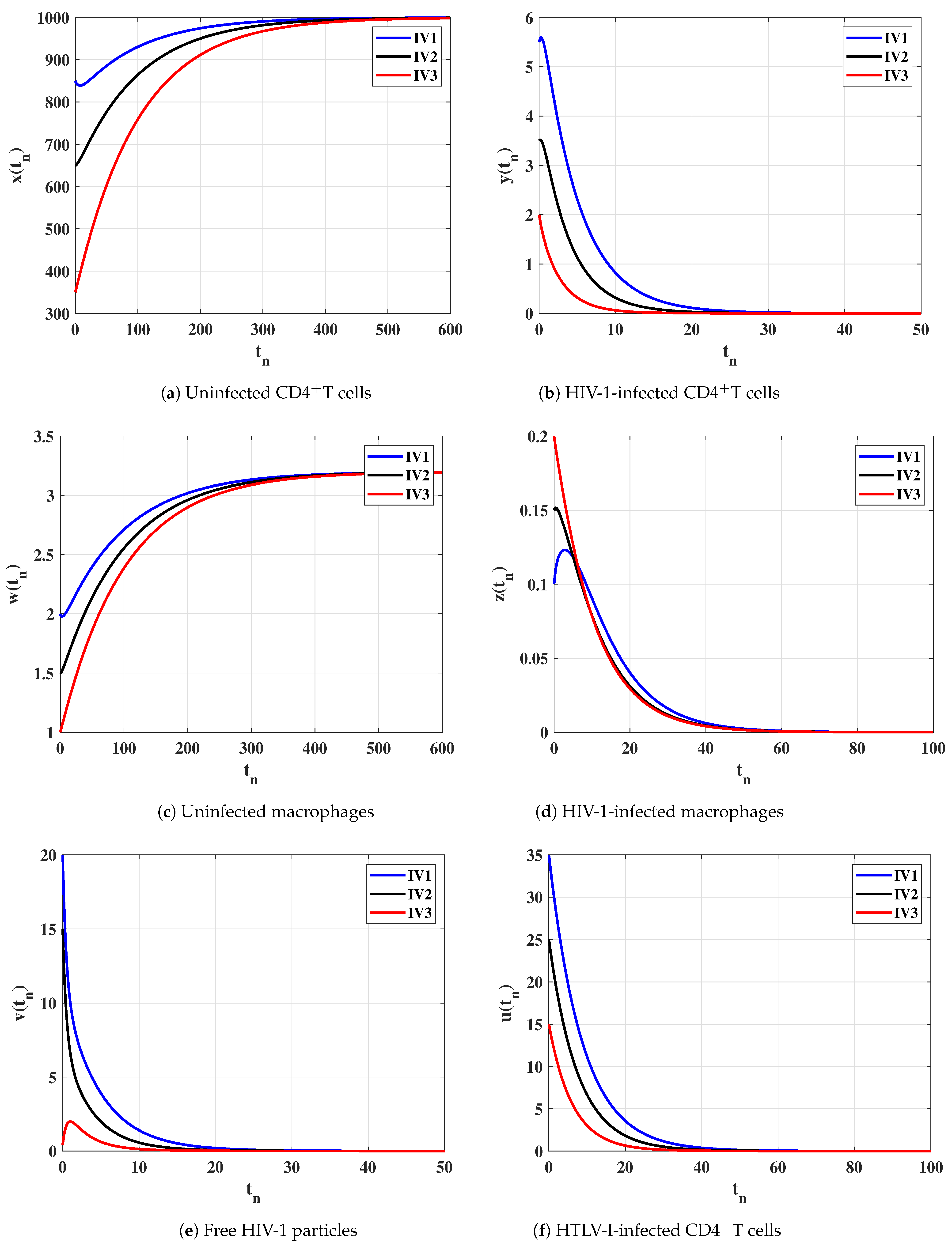
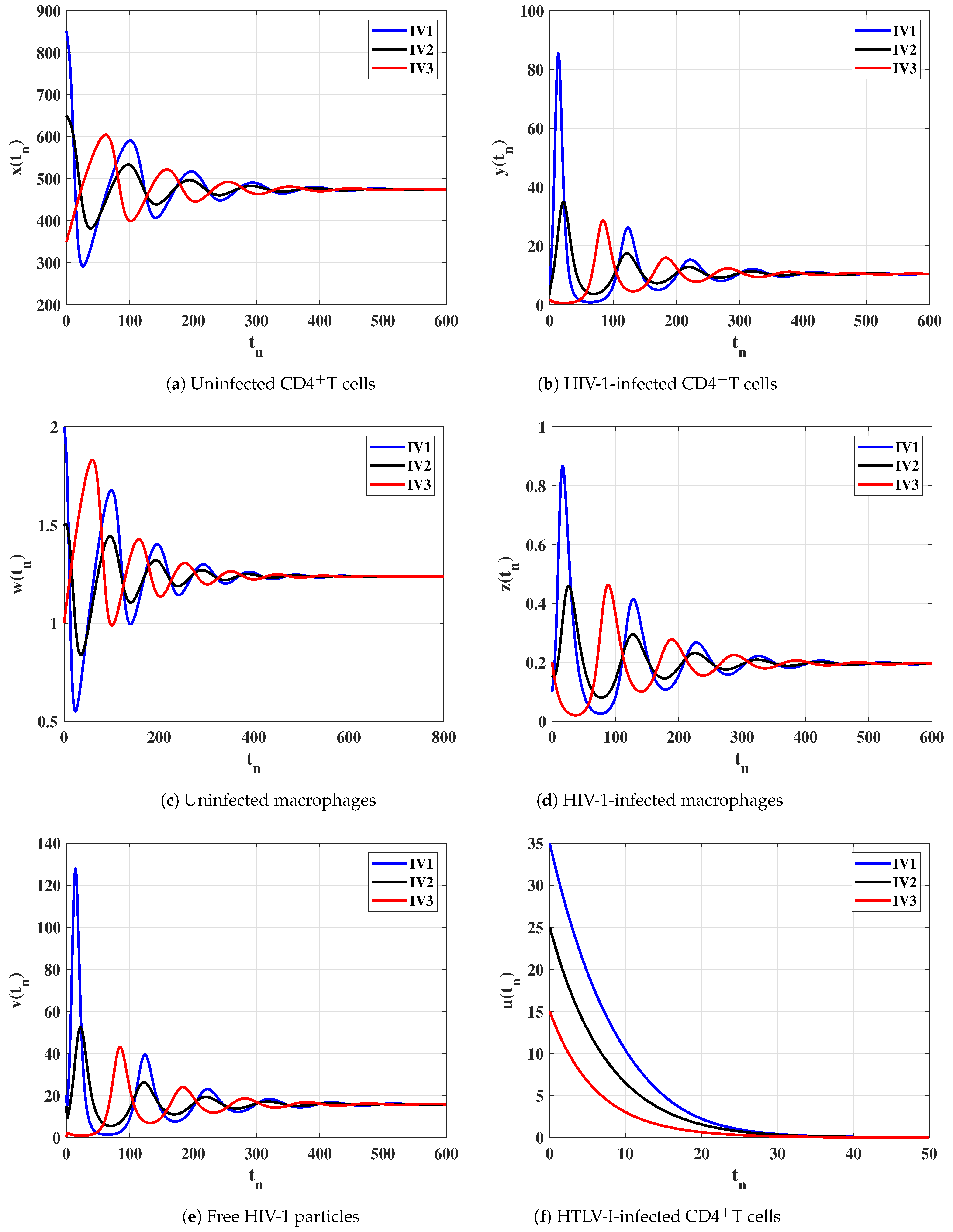
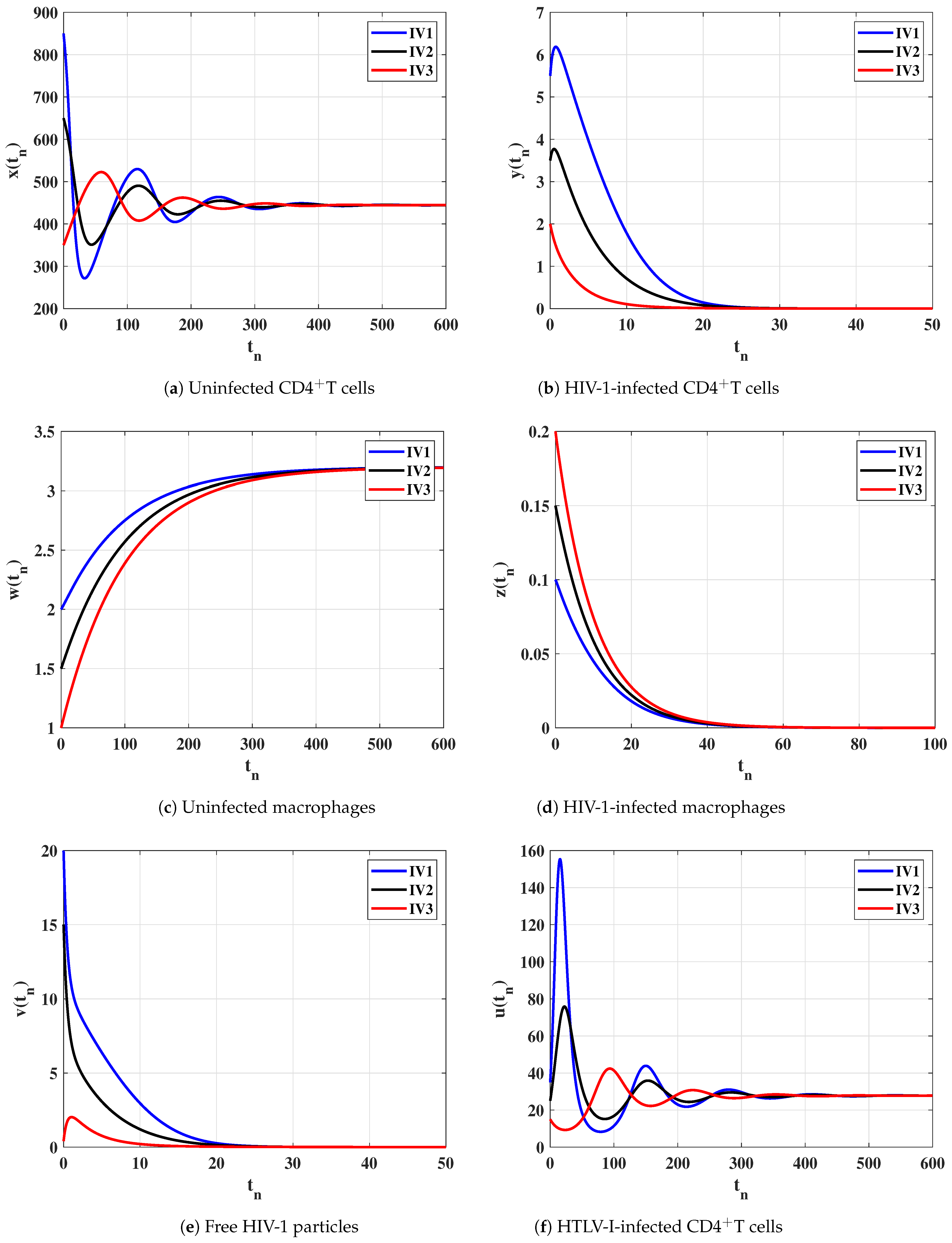
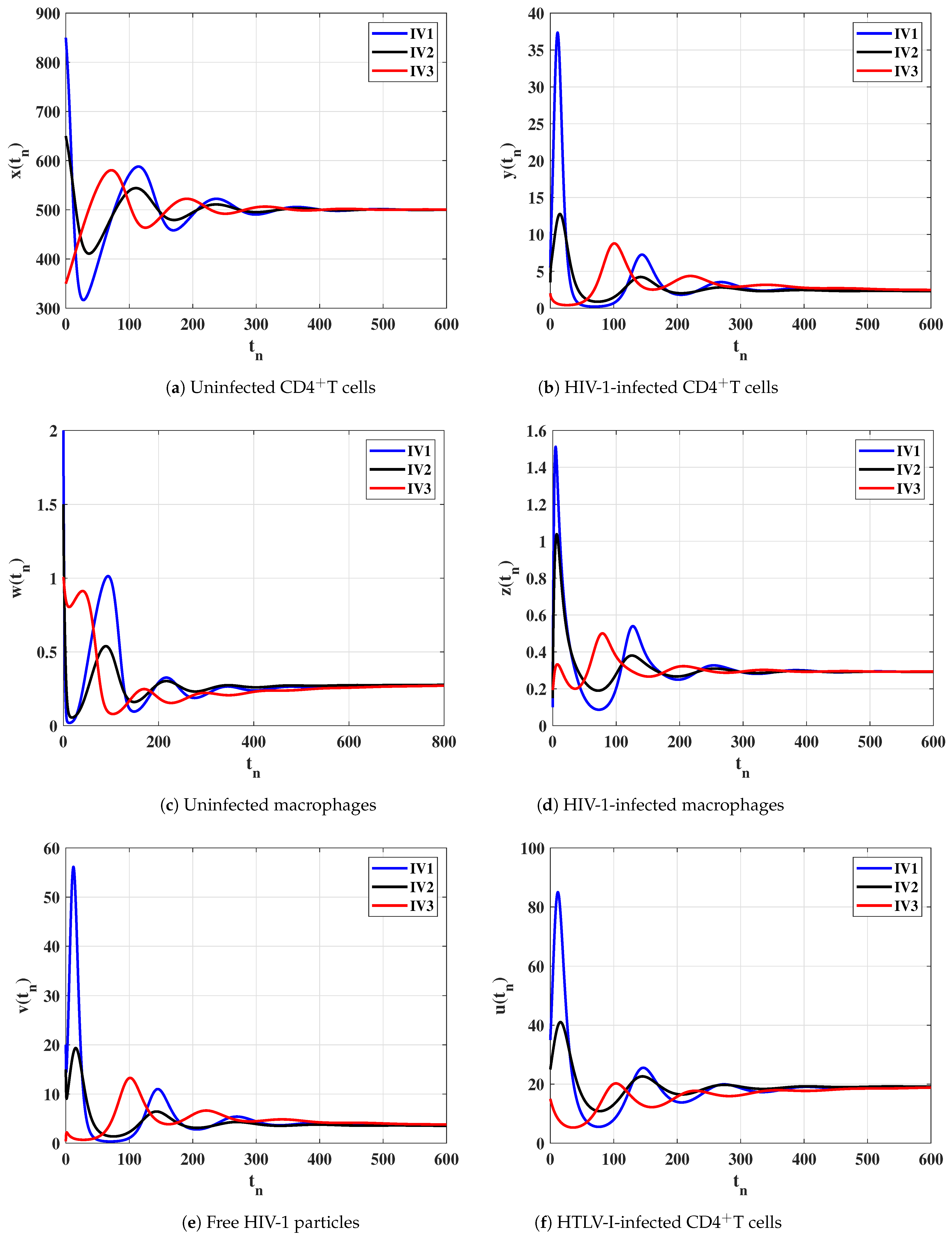
6. Numerical Simulations

To perform numerical simulations for the discrete-time model (10)–(15), we use the data given in Table 1:
We mention that most of these values are taken from previous studies for HIV-1 single-infection and HTLV-I single-infection models, while other values ω 1 , ω 2 and ω 3 are simply assumed to carry out the numerical simulations. Getting real data from HTLV-I and HIV-1 co-infection patients is not easy and needs more experimental works. Therefore, estimating the parameters of the HTLV-I and HIV-1 co-infection model is still open for future work.
To demonstrate the global stability of the discrete-time model’s equilibria given in Theorems 1–4, we show that the solutions of the model converge to one of the four equilibria regardless of the selected initial conditions. Therefore, we choose three different initial values as
IV 1 : x 0 = 850 , y 0 = 5.5 , w 0 = 2 , z 0 = 0.1 , v 0 = 20 , u 0 = 35 , IV 2 : x 0 = 650 , y 0 = 3.5 , w 0 = 1.5 , z 0 = 0.15 , v 0 = 15 , u 0 = 25 , IV 3 : x 0 = 350 , y 0 = 2 , w 0 = 1 , z 0 = 0.2 , v 0 = 0.4 u 0 = 15 .
We choose ω 1 , ω 2 and ω 3 as follows:
Case (I) ω 1 = 0.0002 , ω 2 = 0.001 and ω 3 = 0.0001 . This gives R 0 = 0.6096 1 and R 1 = 0.5 < 1 . Figure 1 illustrates that the concentrations of uninfected CD4 + T cells and uninfected macrophages increase and tend to the healthy values x 0 = 1000 and w 0 = 3.1980 , while the concentrations of other compartments decrease and converge to zero. Therefore, E Q 0 is GAS and this agrees the result of Theorem 1. In this case, both HTLV-I and HIV-1 are cleared.
Case (II) ω 1 = 0.0007 , ω 2 = 0.001 and ω 3 = 0.0001 . These values give R 0 = 2.109 > 1 and R 1 = 0.5 < 1 . From Figure 2, we see that the solutions of the discrete-time model tend to the equilibrium E Q 1 = ( 474.42 , 10.51 , 1.24 , 0.2 , 15.83 , 0 ) . As a result, E Q 1 exists, and based on Theorem 2, it is GAS. This result shows that, the HIV-1 single-infection can be reached for all initial states.
Case (III) ω 1 = 0.0003 , ω 2 = 0.0001 and ω 3 = 0.00045 , and then R 1 = 2.25 > 1 and R 02 + ( R 01 / R 1 ) = 0.401 < 1 . Figure 3 clarifies that the solutions of the discrete-time model reach the equilibrium E Q 2 = ( 444.44 , 0 , 3.198 , 0 , 0 , 27.78 ) for all the initial states. According to Lemma 2 and Theorem 3, E Q 2 exists and it is GAS. This result shows that the HTLV-I single-infection can be reached for all initial states.
Case (IV) ω 1 = 0.00065 , ω 2 = 0.03 and ω 3 = 0.0004 , and thus, R 1 / R 01 = 1.0256 > 1 , R 2 = 11.5128 > 1 and R 3 = 4.3903 > 1 . Figure 4 illustrates that the solutions of the discrete-time model starting with initial values IV1-IV3 converge to the equilibrium E Q 3 = ( 500 , 2.28 , 0.28 , 0.29 , 3.5 , 19.31 ) . Based on Lemma 2 and Theorem 4, E Q 4 exists and it is GAS. This result shows that the HTLV-I and HIV-1 co-infection can be reached for all initial states.
For more confirmation, we examine the local stability of the equilibria of the discrete-time model in cases (I)–(IV). The Jacobian matrix J = J ( x , y , w , z , v , u ) of model (18)–(22) is calculated as
J = J 11 0 0 0 J 15 J 16 J 21 J 22 0 0 J 25 J 26 0 0 J 33 0 J 35 0 0 0 J 43 J 44 J 45 0 J 51 J 52 J 53 J 54 J 55 J 56 J 61 0 0 0 J 65 J 66 ,
where
J 11 = 1 1 + Ω ( h ) ( γ 1 + ω 1 v + ω 3 u ) , J 15 = ω 1 Ω ( h ) ( x + ξ 1 Ω ( h ) ) ( 1 + Ω ( h ) ( γ 1 + ω 1 v + ω 3 u ) ) 2 , J 16 = ω 3 Ω ( h ) ( x + ξ 1 Ω ( h ) ) ( 1 + Ω ( h ) ( γ 1 + ω 1 v + ω 3 u ) ) 2 , J 21 = ω 1 Ω ( h ) v ( 1 + α 1 Ω ( h ) ) ( 1 + Ω ( h ) ( γ 1 + ω 1 v + ω 3 u ) ) , J 22 = 1 1 + α 1 Ω ( h ) , J 25 = ω 1 Ω ( h ) ( x + ξ 1 Ω ( h ) ) ( 1 + γ 1 Ω ( h ) + ω 3 Ω ( h ) u ) ( 1 + α 1 Ω ( h ) ) ( 1 + Ω ( h ) ( γ 1 + ω 1 v + ω 3 u ) ) 2 , J 26 = ω 1 ω 3 Ω ( h ) 2 ( x + ξ 1 Ω ( h ) ) v ( 1 + α 1 Ω ( h ) ) ( 1 + Ω ( h ) ( γ 1 + ω 1 v + ω 3 u ) ) 2 , J 33 = 1 1 + γ 2 Ω ( h ) + ω 2 Ω ( h ) v , J 35 = ω 2 Ω ( h ) ( w + ξ 2 Ω ( h ) ) ( 1 + γ 2 Ω ( h ) + ω 2 Ω ( h ) v ) 2 , J 43 = ω 2 Ω ( h ) v ( 1 + α 2 Ω ( h ) ) ( 1 + γ 2 Ω ( h ) + ω 2 Ω ( h ) v ) , J 44 = 1 1 + α 2 Ω ( h ) , J 45 = ω 2 Ω ( h ) ( 1 + γ 2 Ω ( h ) ) ( w + ξ 2 Ω ( h ) ) ( 1 + α 2 Ω ( h ) ) ( 1 + γ 2 Ω ( h ) + ω 2 Ω ( h ) v ) 2 , J 51 = α 1 β 1 ω 1 Ω 2 ( h ) v ( 1 + α 1 Ω ( h ) ) ( 1 + θ Ω ( h ) ) ( 1 + Ω ( h ) ( γ 1 + ω 1 v + ω 3 u ) ) , J 52 = α 1 β 1 Ω ( h ) ( 1 + α 1 Ω ( h ) ) ( 1 + θ Ω ( h ) ) , J 53 = α 2 β 2 ω 2 Ω 2 ( h ) v ( 1 + α 2 Ω ( h ) ) ( 1 + θ Ω ( h ) ) ( 1 + γ 2 Ω ( h ) + ω 2 Ω ( h ) v ) , J 54 = α 2 β 2 Ω ( h ) ( 1 + α 2 Ω ( h ) ) ( 1 + θ Ω ( h ) ) , J 55 = 1 1 + θ Ω ( h ) + Ω ( h ) 1 + θ Ω ( h ) ω 2 α 2 β 2 Ω ( h ) ( 1 + γ 2 Ω ( h ) ) ( w + ξ 2 Ω ( h ) ) ( 1 + α 2 Ω ( h ) ) ( 1 + γ 2 Ω ( h ) + ω 2 Ω ( h ) v ) 2 + ω 1 α 1 β 1 Ω ( h ) ( x + ξ 1 Ω ( h ) ) ( 1 + γ 1 Ω ( h ) + ω 3 Ω ( h ) u ) ( 1 + α 1 Ω ( h ) ) ( 1 + Ω ( h ) ( γ 1 + ω 1 v + ω 3 u ) ) 2 , J 56 = ω 1 ω 3 α 1 β 1 Ω 3 ( h ) ( x + ξ 1 Ω ( h ) ) v ( 1 + α 1 Ω ( h ) ) ( 1 + θ Ω ( h ) ) ( 1 + Ω ( h ) ( γ 1 + ω 1 v + ω 3 u ) ) 2 , J 61 = Ω ( h ) ω 3 u ( 1 + δ Ω ( h ) ) ( 1 + Ω ( h ) ( γ 1 + ω 1 v + ω 3 u ) ) , J 65 = ω 1 ω 3 Ω 2 ( h ) ( x + ξ 1 Ω ( h ) ) u ( 1 + δ Ω ( h ) ) ( 1 + Ω ( h ) ( γ 1 + ω 1 v + ω 3 u ) ) 2 , J 66 = 1 1 + δ Ω ( h ) 1 + ω 3 Ω ( h ) ( x + ξ 1 Ω ( h ) ) ( 1 + γ 1 Ω ( h ) + ω 1 Ω ( h ) v ) ( 1 + Ω ( h ) ( γ 1 + ω 1 v + ω 3 u ) ) 2 .
Then, we compute the eigenvalues λ j , j = 1 , 2 , , 6 of the matrix J , at each equilibrium. An equilibrium point of the discrete-time model is locally asymptotically stable (LAS) when λ j < 1 , for all j = 1 , 2 , , 6 . We compute the eigenvalues of all nonnegative equilibria using the values of ω 1 , ω 2 and ω 3 given in Cases (I)-(IV). Table 2 contains the nonnegative equilibria, the absolute value of the eigenvalues and whether the equilibrium point is LAS or unstable. We note that when an equilibrium point is GAS, then it is also LAS, and all the other equilibria will be unstable.

7. Conclusions

In this paper, we studied a discrete-time HTLV-I and HIV-1 co-infection model within a host. We discretized the continuous-time co.infection model by using the NSFD scheme. We proved the positivity and ultimate boundedness of the discrete-time model’s solutions. Then, we deduced that the model has four equilibria: infection-free equilibrium E Q 0 , chronic HIV-1 single-infection equilibrium E Q 1 , chronic HTLV-I single-infection equilibrium E Q 2 and chronic HTLV-I/HIV-1 co-infection equilibrium E Q 3 . We showed that the existence and stability of equilibria are determined by four positive threshold parameters R j , j = 0 , 1 , 2 , 3 . The global stability of all equilibria of the discrete-time model was examined by constructing Lyapunov functions. We obtained that E Q 0 is GAS, when R 0 1 and R 1 1 . The equilibrium E Q 1 exists when R 0 > 1 and it is GAS when R 0 > 1 and R 1 1 . When R 1 > 1 , the equilibrium E Q 2 exists and it is GAS if R 1 > 1 and R 02 + R 01 R 1 1 . Finally, we found that the equilibrium E Q 3 exists and it is GAS when R 1 R 01 > 1 , R 2 > 1 and R 3 > 1 . We simulated the discrete-time model to confirm the theoretical results.
The model addressed in this article can be extended in several directions by including (i) time delay [5], (ii) memory effects [28], (iii) reaction–diffusion [53], and (iv) stochastic interactions [54]. These points are left for future works.

Author Contributions

Conceptualization, A.M.E. and A.K.A.; Formal analysis, A.M.E., A.K.A. and A.D.H.; Investigation, A.M.E. and A.K.A.; Methodology, A.M.E. and A.D.H.; Writing—original draft, A.K.A.; Writing—review & editing, A.M.E. and A.K.A. All authors have read and agreed to the published version of the manuscript.

Funding

This Project was funded by the Deanship of Scientific Research (DSR) at King Abdulaziz University, Jeddah, under grant no. (G: 1436-130-125).

Data Availability Statement

Not applicable.

Acknowledgments

This Project was funded by the Deanship of Scientific Research (DSR) at King Abdulaziz University, Jeddah, under grant no. (G: 1436-130-125). The authors, therefore, acknowledge with thanks DSR for technical and financial support.

Conflicts of Interest

The authors declare no conflict of interest.

References

  1. Ciupe, S.M.; Heffernan, J.M. In-host modeling. Infect. Dis. Model. 2017, 2, 188–202. [Google Scholar] [CrossRef]
  2. Nowak, M.A.; Bangham, C.R.M. Population dynamics of immune responses to persistent viruses. Science 1996, 272, 74–79. [Google Scholar] [CrossRef] [PubMed]
  3. Wang, X.; Song, X.; Tang, S.; Rong, L. Dynamics of an HIV model with multiple infection stages and treatment with different drug classes. Bull. Math. Biol. 2016, 78, 322–349. [Google Scholar] [CrossRef] [PubMed]
  4. Perelson, A.S.; Essunger, P.; Cao, Y.; Vesanen, M.; Hurley, A.; Saksela, K.; Markowitz, M.; Ho, D.D. Decay characteristics of HIV-1-infected compartments during combination therapy. Nature 1997, 387, 188–191. [Google Scholar] [CrossRef]
  5. Nelson, P.W.; Perelson, A.S. Mathematical analysis of delay differential equation models of HIV-1 infection. Math. Biosci. 2002, 179, 73–94. [Google Scholar] [CrossRef]
  6. Nelson, P.W.; Murray, J.D.; Perelson, A.S. A model of HIV-1 pathogenesis that includes an intracellular delay. Math. Biosci. 2000, 163, 201–215. [Google Scholar] [CrossRef]
  7. Perelson, A.S.; Nelson, P.W. Mathematical analysis of HIV-1 dynamics in vivo. SIAM Rev. 1999, 41, 3–44. [Google Scholar] [CrossRef]
  8. Lin, J.; Xu, R.; Tian, X. Threshold dynamics of an HIV-1 model with both viral and cellular infections, cell-mediated and humoral immune responses. Math. Biosci. Eng. 2018, 16, 292–319. [Google Scholar] [CrossRef]
  9. Gao, Y.; Wang, J. Threshold dynamics of a delayed nonlocal reaction-diffusion HIV infection model with both cell-free and cell-to-cell transmissions. J. Math. Anal. Appl. 2020, 488, 124047. [Google Scholar] [CrossRef]
  10. Feng, T.; Qiu, Z.; Meng, X.; Rong, L. Analysis of a stochastic HIV-1 infection model with degenerate diffusion. Appl. Math. Comput. 2019, 348, 437–455. [Google Scholar] [CrossRef]
  11. Callaway, D.S.; Perelson, A.S. HIV-1 infection and low steady state viral loads. Bull. Math. Biol. 2002, 64, 29–64. [Google Scholar] [CrossRef] [PubMed]
  12. Adams, B.M.; Banks, H.T.; Kwon, H.D.; Tran, H.T. Dynamic multidrug therapies for HIV: Optimal and STI control approaches. Math. Biosci. Eng. 2004, 1, 223–241. [Google Scholar] [CrossRef] [PubMed]
  13. Adams, B.M.; Banks, H.T.; Davidian, M.; Kwon, H.D.; Tran, H.T.; Wynne, S.N.; Rosenberg, E.S. HIV dynamics: Modeling, data analysis, and optimal treatment protocols. J. Comput. Appl. Math. 2005, 184, 10–49. [Google Scholar] [CrossRef]
  14. Qi, K.; Jiang, D.; Hayat, T.; Alsaedi, A. Virus dynamic behavior of a stochastic HIV/AIDS infection model including two kinds of target cell infections and CTL immune. Math. Comput. Simul. 2021, 188, 548–570. [Google Scholar] [CrossRef]
  15. Lim, A.G.; Maini, P.K. HTLV-I infection: A dynamic struggle between viral persistence and host immunity. J. Theor. Biol. 2014, 352, 92–108. [Google Scholar] [CrossRef]
  16. Li, M.Y.; Shu, H. Multiple stable periodic oscillations in a mathematical model of CTL response to HTLV-I infection. Bull. Math. Biol. 2011, 73, 1774–1793. [Google Scholar] [CrossRef] [PubMed]
  17. Wang, W.; Ma, W. Global dynamics of a reaction and diffusion model for an HTLV-I infection with mitotic division of actively infected cells. J. Appl. Anal. Comput. 2017, 7, 899–930. [Google Scholar] [CrossRef]
  18. Li, F.; Ma, W. Dynamics analysis of an HTLV-1 infection model with mitotic division of actively infected cells and delayed CTL immune response. Math. Methods Appl. Sci. 2018, 41, 3000–3017. [Google Scholar] [CrossRef]
  19. Wang, Y.; Liu, J.; Heffernan, J.M. Viral dynamics of an HTLV-I infection model with intracellular delay and CTL immune response delay. J. Math. Anal. Appl. 2018, 459, 506–527. [Google Scholar] [CrossRef]
  20. Wang, L.; Liu, Z.; Li, Y.; Xu, D. Complete dynamical analysis for a nonlinear HTLV-I infection model with distributed delay, CTL response and immune impairment. Discret. Contin. Dyn. Ser. B 2020, 25, 917–933. [Google Scholar] [CrossRef] [Green Version]
  21. Chenar, F.F.; Kyrychko, Y.N.; Blyuss, K.B. Mathematical model of immune response to hepatitis B. J. Theor. Biol. 2018, 447, 98–110. [Google Scholar] [CrossRef]
  22. Kitagawa, K.; Kuniya, T.; Nakaoka, S.; Asai, Y.; Watashi, K.; Iwami, S. Mathematical Analysis of a Transformed ODE from a PDE Multiscale Model of Hepatitis C Virus Infection. Bull. Math. 2019, 81, 1427–1441. [Google Scholar] [CrossRef]
  23. Baccam, P.; Beauchemin, C.; Macken, C.A.; Hayden, F.G.; Perelson, A.S. Kinetics of influenza A virus infection in humans. J. Virol. 2006, 80, 7590–7599. [Google Scholar] [CrossRef]
  24. Nuraini, N.; Tasman, H.; Soewono, E.; Sidarto, K.A. A with-in host dengue infection model with immune response. Math. Comput. Model. 2009, 49, 1148–1155. [Google Scholar] [CrossRef]
  25. Wang, Y.; Liu, X. Stability and Hopf bifurcation of a within-host chikungunya virus infection model with two delays. Math. Comput. Simul. 2017, 138, 31–48. [Google Scholar] [CrossRef]
  26. Nguyen, V.K.; Binder, S.C.; Boianelli, A.; Meyer-Hermann, M.; Hernandez-Vargas, E.A. Ebola virus infection modelling and identifiability problems. Front. Microbiol. 2015, 6, 257. [Google Scholar] [CrossRef]
  27. Hernandez-Vargas, E.A.; Velasco-Hernandez, J.X. In-host mathematical modelling of COVID-19 in humans. Annu. Rev. Control 2020, 50, 448–456. [Google Scholar] [CrossRef]
  28. Chatterjee, A.N.; Basir, F.A.; Almuqrin, M.A.; Mondal, J.; Khan, I. SARS-CoV-2 infection with lytic and nonlytic immune responses: A fractional order optimal control theoretical study. Results Phys. 2021, 26, 104260. [Google Scholar] [CrossRef]
  29. Elaiw, A.M.; Alsulami, R.S.; Hobiny, A.D. Modeling and stability analysis of within-host IAV/SARS-CoV-2 coinfection with antibody immunity. Mathematics 2022, 10, 4382. [Google Scholar] [CrossRef]
  30. Elaiw, A.M.; Elnahary, E.K. Analysis of general humoral immunity HIV dynamics model with HAART and distributed delays. Mathematics 2019, 7, 157. [Google Scholar] [CrossRef] [Green Version]
  31. Elaiw, A.M.; AlShamrani, N.H. Analysis of a within-host HTLV-I/HIV-1 co-infection model with immunity. Virus Res. 2021, 295, 1–23. [Google Scholar] [CrossRef] [PubMed]
  32. Elaiw, A.M.; AlShamrani, N.H. HTLV/HIV dual Infection: Modeling and analysis. Mathematics 2021, 9, 51. [Google Scholar] [CrossRef]
  33. Elaiw, A.M.; AlShamrani, N.H.; Dahy, E.; Abdellatif, A. Stability of within host HTLV-I/HIV-1 co-infection in the presence of macrophages. Int. J. Biomath. 2022, 16, 2250066. [Google Scholar] [CrossRef]
  34. Pasha, S.A.; Nawaz, Y.; Arif, M.S. On the nonstandard finite difference method for reaction–diffusion models. Chaos Solitons Fractals 2023, 166, 112929. [Google Scholar] [CrossRef]
  35. Maamar, M.H.; Ehrhardt, M.; Tabharit, L. A Nonstandard Finite Difference Scheme for a Time-Fractional Model of Zika Virus Transmission. 2022. Available online: https://www.imacm.uni-wuppertal.de/fileadmin/imacm/preprints/2022/imacm_22_21.pdf (accessed on 20 December 2022).
  36. Farooqi, A.; Ahmad, R.; Alotaibi, H.; Nofal, T.A.; Farooqi, R.; Khan, I. A comparative epidemiological stability analysis of predictor corrector type non-standard finite difference scheme for the transmissibility of measles. Results Phys. 2021, 21, 103756. [Google Scholar] [CrossRef]
  37. Mickens, R.E. Nonstandard Finite Difference Models of Differential Equations; World Scientific: Singapore, 1994. [Google Scholar]
  38. Mickens, R.E. Applications of Nonstandard Finite Difference Schemes; World Scientific: Singapore, 2000. [Google Scholar]
  39. Treibert, S.; Brunner, H.; Ehrhardt, M. A nonstandard finite difference scheme for the SVICDR model to predict COVID-19 dynamics. Math. Biosci. Eng. 2022, 19, 1213–1238. [Google Scholar]
  40. Korpusik, A. A nonstandard finite difference scheme for a basic model of cellular immune response to viral infection. Commun. Nonlinear Sci. Numer. Simul. 2017, 43, 369–384. [Google Scholar] [CrossRef]
  41. Yang, Y.; Xinsheng, M.; Yahui, L. Global stability of a discrete virus dynamics model with Holling type-II infection function. Math. Methods Appl. Sci. 2016, 39, 2078–2082. [Google Scholar] [CrossRef]
  42. Geng, Y.; Xu, J.; Hou, J. Discretization and dynamic consistency of a delayed and diffusive viral infection model. Appl. Math. Comput. 2018, 316, 282–295. [Google Scholar] [CrossRef]
  43. Vaz, S.; Torres, D.F.M. Discrete-time system of an intracellular delayed HIV model with CTL immune response. arXiv 2022, arXiv:2205.02199. [Google Scholar]
  44. Salman, S.M. A nonstandard finite difference scheme and optimal control for an HIV model with Beddington-DeAngelis incidence and cure rate. Eur. Phys. J. Plus 2020, 135, 808. [Google Scholar] [CrossRef]
  45. Liu, X.L.; Zhu, C.C. A non-standard finite difference scheme for a diffusive HIV-1 infection model with immune response and intracellular delay. Axioms 2022, 11, 129. [Google Scholar] [CrossRef]
  46. Elaiw, A.M.; Alshaikh, M.A. Stability preserving NSFD scheme for a general virus dynamics model with antibody and cell-mediated responses. Chaos Solitons Fractals 2020, 138, 109862. [Google Scholar] [CrossRef]
  47. Elaiw, A.M.; Alshaikh, M.A. Stability of discrete-time HIV dynamics models with three categories of infected CD4+ T-cells. Adv. Differ. Equ. 2019, 2019, 407. [Google Scholar] [CrossRef]
  48. Mickens, R.E. Calculation of denominator functions for nonstandard finite difference schemes for differential equations satisfying apositivity condition. Numer. Methods Partial. Differ. Equ. 2007, 23, 672–691. [Google Scholar] [CrossRef]
  49. Shi, P.; Dong, L. Dynamical behaviors of a discrete HIV-1 virus model with bilinear infective rate. Math. Methods Appl. Sci. 2014, 37, 2271–2280. [Google Scholar] [CrossRef]
  50. Perelson, A.S.; Kirschner, D.E.; de Boer, R. Dynamics of HIV Infection of CD4+ T cells. Math. Biosci. 1993, 114, 81–125. [Google Scholar] [CrossRef]
  51. Mohri, H.; Bonhoeffer, S.; Monard, S.; Perelson, A.S.; Ho, D. Rapid turnover of T lymphocytes in SIV-infected rhesus macaques. Science 1998, 279, 1223–1227. [Google Scholar] [CrossRef]
  52. Elaiw, A.M.; Raezah, A.A.; Azoz, S.A. Stability of delayed HIV dynamics models with two latent reservoirs and immune impairment. Adv. Differ. Equ. 2018, 50, 1–25. [Google Scholar] [CrossRef]
  53. Bellomo, N.; Outada, N.; Soler, J.; Tao, Y.; Winkler, M. Chemotaxis and cross diffusion models in complex environments: Modeling towards a multiscale vision. Math. Model. Methods Appl. Sci. 2022, 32, 713–792. [Google Scholar] [CrossRef]
  54. Gibelli, L.; Elaiw, A.M.; Alghamdi, M.A.; Althiabi, A.M. Heterogeneous population dynamics of active particles: Progression, mutations, and selection dynamics. Math. Model. Methods Appl. Sci. 2017, 27, 617–640. [Google Scholar] [CrossRef]
Figure 1. Solutions of model (10)–(15) with initial conditions IV1–IV3 in case of R 0 1 and R 1 1 .
Axioms 12 00201 g001
Figure 2. Solutions of model (10)–(15) with initial conditions IV1-IV3 in case of R 0 > 1 and R 1 1 .
Axioms 12 00201 g002
Figure 3. Solutions of model (10)–(15) with initial conditions IV1–IV3 in case of R 1 > 1 and R 02 + R 01 R 1 1 .
Axioms 12 00201 g003
Figure 4. Solutions of model (10)–(15) with initial conditions IV1–IV3 in case of R 1 R 01 > 1 , R 2 > 1 and R 3 > 1 .
Axioms 12 00201 g004
Table 1. Model parameters.
ParameterValueSourceParameterValueSourceParameterValueSource
ξ 1 10[18,50] γ 1 0.01 [11,51] θ 2[32]
ξ 2 0.03198 [12,13] γ 2 0.01 [12,13] δ 0.2 [17,32]
α 1 0.5 [6,7] β 1 6[52]h 0.1 [46]
α 2 0.1 [32,52] β 2 6[52] ω 1 , ω 2 , ω 3 VariedAssumed
Table 2. Local stability of equilibria.
CaseSteady State λ j , j = 1 , 2 , , 6 Stability
Case (I) E Q 0 = 1000 , 0 , 3.20 , 0 , 0 , 0 0.999 , 0.999 , 0.991 , 0.990 , 0.983 , 0.807 LAS
Case (II) E Q 0 = 1000 , 0 , 3.20 , 0 , 0 , 0 E Q 1 = ( 474.42 , 10.51 , 1.24 , 0.2 , 15.83 , 0 ) 1.037 , 0.999 , 0.999 , 0.990 , 0.990 , 0.765 0.999 , 0.999 , 0.997 , 0.990 , 0.985 , 0.794 unstable LAS
Case (III) E Q 0 = 1000 , 0 , 3.20 , 0 , 0 , 0 E Q 2 = ( 444.44 , 0 , 3.198 , 0 , 0 , 27.78 ) 1.025 , 0.999 , 0.999 , 0.996 , 0.990 , 0.797 0.999 , 0.999 , 0.999 , 0.990 , 0.974 , 0.815 unstable LAS
Case (IV) E Q 0 = 1000 , 0 , 3.20 , 0 , 0 , 0 E Q 1 = 509.57 , 9.81 , 0.07 , 0.31 , 14.81 , 0 E Q 2 = 500 , 0 , 3.20 , 0 , 0 , 25 E Q 3 = ( 500 , 2.28 , 0.28 , 0.29 , 3.5 , 19.31 ) 1.036 , 1.02 , 0.999 , 0.999 , 0.988 , 0.768 1.0004 , 0.999 , 0.999 , 0.990 , 0.957 , 0.794 1.006 , 0.999 , 0.999 , 0.999 , 0.985 , 0.793 0.999 , 0.999 , 0.999 , 0.992 , 0.987 , 0.794 unstable unstable unstable LAS
Disclaimer/Publisher’s Note: The statements, opinions and data contained in all publications are solely those of the individual author(s) and contributor(s) and not of MDPI and/or the editor(s). MDPI and/or the editor(s) disclaim responsibility for any injury to people or property resulting from any ideas, methods, instructions or products referred to in the content.

