Article

Aggregative Game for Distributed Charging Strategy of PEVs in a Smart Charging Station

Chongqing Key Laboratory of Nonlinear Circuits and Intelligent Information Processing, College of Electronic and Information Engineering, Southwest University, Chongqing 400715, China
*
Author to whom correspondence should be addressed.
Axioms 2023, 12(2), 186; https://doi.org/10.3390/axioms12020186
Submission received: 16 January 2023 / Revised: 8 February 2023 / Accepted: 9 February 2023 / Published: 10 February 2023
(This article belongs to the Special Issue Applied Mathematics in Energy and Mechanical Engineering)

Abstract

:
This paper proposes a charging strategy for plug-in electric vehicles (PEVs) in a smart charging station (SCS) that considers load constraints and time anxieties. Due to the rapidly growing load demand of PEVs and the load capacity investments in infrastructure, PEV charging needs to be subject to overload limits, beyond which failures can occur. The time anxiety is presented to address some of the uncertainties that may arise while charging PEVs. Under an aggregative game framework, this paper constructs a price-driven charging model to minimize costs by choosing the optimal charging strategy. Meanwhile, since the driver information is an aggregated item in the PEV cost function, the drivers’ privacy can be protected. Then, a distributed reflected forward–backward (RFB) splitting method is developed to search for the generalized Nash equilibria (GNE) of the game. The convergence of the proposed algorithm and the effectiveness of the charging strategy are verified by the detailed simulation and results.

1. Introduction

Governments worldwide are promoting plug-in electric vehicles (PEVs) as a clean alternative to conventional gasoline vehicles due to the depletion of fossil fuel resources and environmental pollution, both of which are serious issues. Compared with the conventional gasoline vehicle, the PEV reduces carbon dioxide emissions and the overall operating cost [1]. However, with the rapid growth of PEVs, the total charging load of PEVs entering the electric grid has increased [2], which leads to an overload of charging stations. According to [3], uncoordinated PEV charging lowers the electrical grid’s power quality. However, the demand presented in [4] might actually flatten as a result of the coordinated charging of PEVs. To increase the electric grid’s operational effectiveness and security, we must formulate effective charging strategies to coordinate and control the charging behavior of PEV drivers.
Since PEVs are capable of storing electrical energy, some PEVs can be used as energy suppliers and transmit power in both directions, to and from a smart charging station (SCS), which can mitigate the effects of overcharging at SCS at peak times. Meanwhile, in order to improve the accuracy of the charging strategy, the driver’s time anxiety needs to be taken into account, in addition to the plug-in electric vehicle factor. The authors of Vatanparvar et al. [5] introduced the concept of demand–price elasticity to address the demand–response model based on the drivers’ behavior. A robust-index method was developed in [6] to resolve driver behavior uncertainties and minimize violations to comfort in household load scheduling. In [7], a distributed method was proposed and a means of reducing the impact of some uncertain events under a non-cooperative game was proposed.However, some of these driver behavior models were homogeneous and lacked theoretical justification. In order to improve the validity of the model, four different PEV driver behaviors were proposed to study the effect of time anxiety on plug-in electric vehicle charging. There are two main classes of control architecture in this charging strategy, namely the centralized and distributed approaches.
The authors of Yan et al. [8] proposed a four-stage optimal control method for electric vehicle charging stations (EVCSs) to reduce operating costs and maintain the supply–demand power balance. In [9], a centralized control approach based on multistage droop control was used to operate an island microgrid in the presence of high PEV penetration. Furthermore, the model in [10] utilized a centralized real-time charging scheme based on a convex relaxation method to coordinate PEV charging. However, in the centralized strategy, each driver, as well as the control center, needs to know the complete information, including cost function, local feasible decision sets and affine sharing constraints, which can easily compromise the drivers’ privacy. Meanwhile, in many cases, no central node can communicate with all drivers in both directions, and it is not possible to realize large-scale driver communication in a real-time manner. Therefore, a distributed strategy is used to compute the local decisions corresponding to PEVs and generalized Nash equilibria and communicate with the adjacent local decisions using the drivers’ local data, which reduces the computational and interaction burden and maintains the privacy of driver information. Based on a decentralized protocol, Li et al. [11] presented a charge control technique for large-scale PEVs under the Newton-type algorithm. The authors of Gan et al. [12] studied a decentralized algorithm to optimize PEV charging during off-peak hours. However, the distributed algorithm described above rarely considers the strategic interaction between multiple PEVs in the charging station.
Therefore, to study communication between multiple PEVs, we then focused on game theory, as this is a powerful tool for analyzing the interactions between multiple decision makers and can improve the model’s performance. Since the famous Cournot model was proposed, aggregative games have become an important type of game theory. In the description for the aggregative game in [13], each driver was not subject to a one-to-one interaction, but was subject to a number of aggregations across the charging strategy. Recent studies in [14,15,16,17] considered the linear aggregation functions and quadratic cost functions in such games, as well as their interaction with plug-in electric vehicle charging. Based on the literature, a distributed reflected forward–backward splitting method was proposed in [18] to find the generalized Nash equilibria of the aggregative game. Unlike the distributed algorithm presented above, this algorithm exploits the aggregated coupling structure in the cost function, meaning that each agent only needs to exchange and maintain an aggregated estimate, not including the estimate of the even multiplier, reducing the computational and communication burden of the model. In addition, since each PEV only shares its estimate of the total, it does not need to share the complete information, further protecting the privacy of the drivers. The main contributions of this paper are summarized as follows:
(1)
A new price-driven charging model combining time anxiety and load constraints is constructed to minimize the cost of an individual PEV driver within the framework of an aggregative game. In particular, as everyone only knows the final summation result, not the specific information, the aggregation game can better protect the privacy of drivers.
(2)
Load constraints are proposed to protect the safety of SCS. Then, four PEV driver behaviors are proposed based on different time anxiety states and load constraints. Meanwhile, the effects of time anxiety under four different driver behaviors are compared, and the effects of uncertain occurrence events are reduced by the charging strategy.
(3)
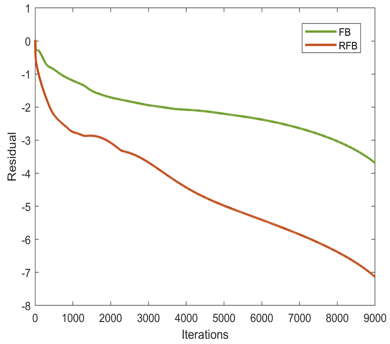
A distributed reflected forward–backward algorithm is designed to seek the generalized Nash equilibria of the model. The proposed algorithm seeks its optimal response charging strategy regarding the current load and time anxiety in the electric grid, thus preventing overload in the smart charging station and mitigating the impact of uncertain events that may occur at the PEV charging time. The algorithm obtains an improvement in significant convergence compared to the numerical values of the FB algorithm [19].

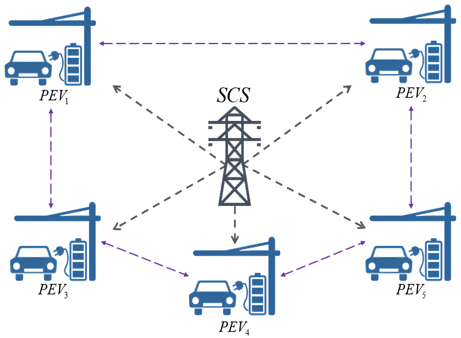
2. System Model and Problem Formulation

As this paper focuses on charging PEVs, the studied system is named SCS, which is considered to be part of the electric grid. In [20,21,22], SCS is composed of PEVs, which are powered by the electric grid, and the PEV can transmit power in both directions between the electric grid. Meanwhile, each PEV i ( i I = 1 , 2 , , N ) is the electric grid user in Figure 1. We define d t as the basic demand load of the system at time t. Let vector x i = col ( x i , 1 , , x i , T ) denote the charging curve of PEV i over all the time slots and x i , t define the charging power of PEV i at time t. In the SCS, the driver can query the electrical grid constraint described in Figure 1 to prevent the required cost from exceeding the load. Moreover, as different drivers have different needs, they may have a preference for a particular charging time, as they encounter various forms of uncertainty, i.e., events that may occur at a later charging time; therefore, they may feel an urge to finish charging the PEV earlier. Therefore, each PEV in SCS can be charged flexibly based on the available information, which can meet the demand and reduce the charging cost.

2.1. Feasible Charging Coordination Constraint Profiles

2.1.1. Battery Capacity Constraint for PEV i

We describe the battery dynamics of PEV i using a linear model (1), in which π i t represents the state of charge of PEV i at time t. Meanwhile, π i min denotes the lower limit of battery capacity and π i max denotes the upper limit of battery capacity for PEV i:
π i t + 1 = π i t + x i , t , π i min π i t π i max

2.1.2. Charging Constraint for PEVs

For each PEV i, the total electrical energy that it obtains needs to meet its charging requirement needs. Based on this constraint, let R i be the required electrical energy. Therefore, the following equation holds:
t = 1 T x i , t = R i
Moreover, each PEV i can choose to charge and discharge according to its situation, which depends on the PEV battery capacity. Note here that PEVs cannot be selected for charging or discharging at the same time; only one of them can be selected. x i ̲ is defined as the minimum discharging power of a PEV i, and x i ¯ is defined as the maximum charging power of a PEV i:
x i ̲ x i , t x i ¯

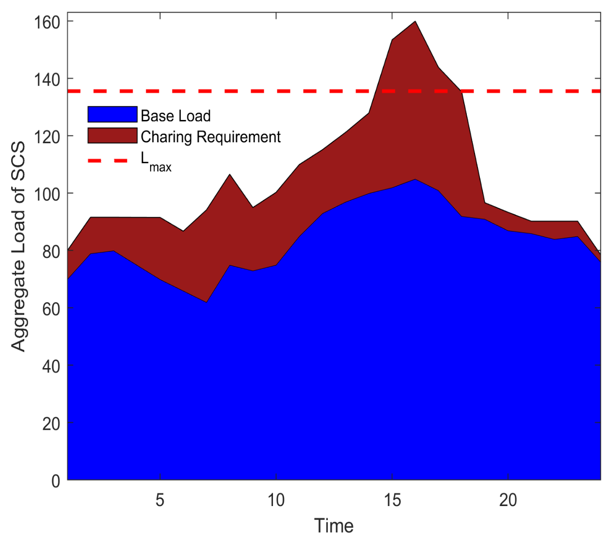
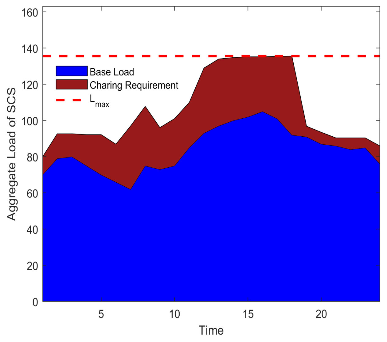
2.1.3. Overload Constraint for Charging PEVs

To avoid overloading the SCS, the charging demand of all the PEVs cannot exceed the maximum electrical energy supplied by the SCS. Let C max denote the total PEV load, and the basic demand load at moment t is set to d t , which denotes the basic electrical load transmitted through the SCS at time t. As the constraint spatially couples the charging demand of all PEVs using the SCS at time t, constraint (4) is referred to as a joint constraint:
i = 1 N x i , t + d t C max

2.1.4. Feasible Charging Profiles

We assume that the set X i is the feasible charging profile and X i is a nonempty, compact convex set. Let X = x 1 , x 2 , , x N x i X i , i I denote the set of charging profiles of all PEVs. Then, X is also nonempty, compact and convex. Therefore, set X i can be written as follows:
X i = x i ( 1 ) ( 2 ) ( 3 ) ( 4 )

2.2. Cost Function of PEVs

We assume that there are N drivers, in which r ( r N ) start at the charging time and enter a state of anxiety after a period of time. For PEV i, t i a is denoted as the arrival time to the SCS and t i d as the departure time at which SCS will be left; the discharge is no longer considered after anxiety begins. Considering the aggregative game framework, we defined σ ( x ) = 1 N i = 1 N x i , and the minimization cost function of PEV i under the corresponding energy consumption constraint is defined as follows:
min x i f i x i , σ ( x ) = t = 1 T S i , t 0 x i , t ρ t d t + μ i , t + j i x j , t d μ i , t
in which S i , t denotes the driver’s anxiety influence at time t. Next, the pricing function ρ t ( L t ) is defined
ρ t L t = α t L t + β t min x i f i x i , σ ( x ) = t = 1 T S i , t 0 x i , t α t d t + μ i , t + j i x j , t + β t d μ i , t
where L t = d t + μ i , t + j i x j , t represents the total load at time t. The pricing function is for a nonlinear form that varies with the increasing charging load of PEV i, while the models in [23,24] use ρ t as a linear function. As a consequence, the linearly decreasing marginal benefits [12,23,24] correspond to the PEV quadratic pricing function. In the meantime, the PEV i increases a load of μ i , t to the electricity grid at time t; the driver of PEV pays an amount of ρ t d t + μ i , t + j i x j , t Δ μ i , t for charging at the time t. When Δ μ i , t tends toward zero and μ i , t changes from zero to x i , t , it then evolves into Formula (8):
min x i f i x i , σ ( x ) = d + N σ ( x ) 1 2 x i T S i α x i + 1 T T S i β x i

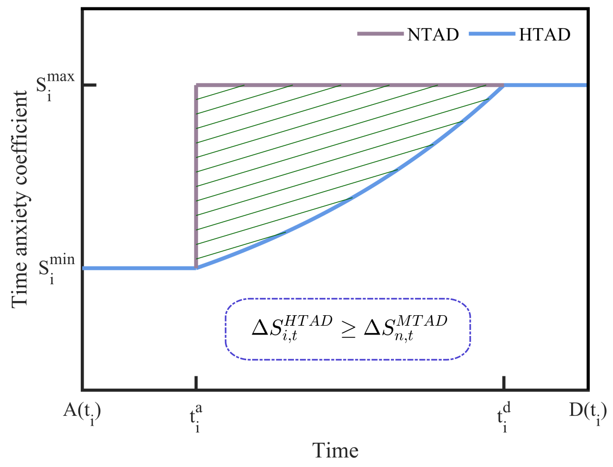
2.3. Time Anxiety for Drivers
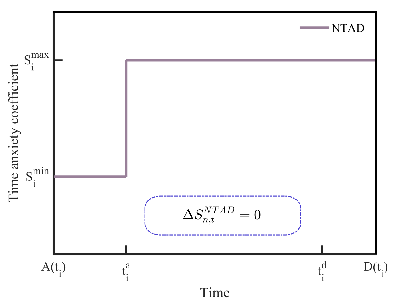
The design of the cost function (8) shows that a higher price leads to lower charging power. Furthermore, if the driver has time anxiety about charging and discharging the PEV, the charging power needs to be higher. Based on this conclusion, S i , t must be small to have a high charging power. Following that, at the time of charging, the value of S i , t gradually rises. Meanwhile, the local objective function was defined according to the problem of anxious and non-anxious drivers, so we obtained two different settings.
The first setting is non-anxious drivers, and we defined S as a constant. This means that the driver has a constant anxiety factor at the charging time, which does not change over time. In this model, we denoted A T ( i ) as the arrival time of PEV i to SCS and denoted D T ( i ) as the departure time of PEV i from SCS:
S i , t = S , A T ( i ) t < D T ( i ) 0 , otherwise
and the next setting is anxious drivers. We defined V i , t as the ratio of the duration of the anxiety state to the overall anxiety time. Thus, the following equation holds:
V i , t = t t i a t i d t i a , t i a t < t i d
With the time anxiety studied in this paper, at the time from A T ( i ) to t i a , the time anxiety is at its lowest value S i , min , and from t i d to D T ( i ) , it is at its highest value S i , max . This paper will explore the behavior of PEV drivers based on [7] and propose four different behaviors:
(1)
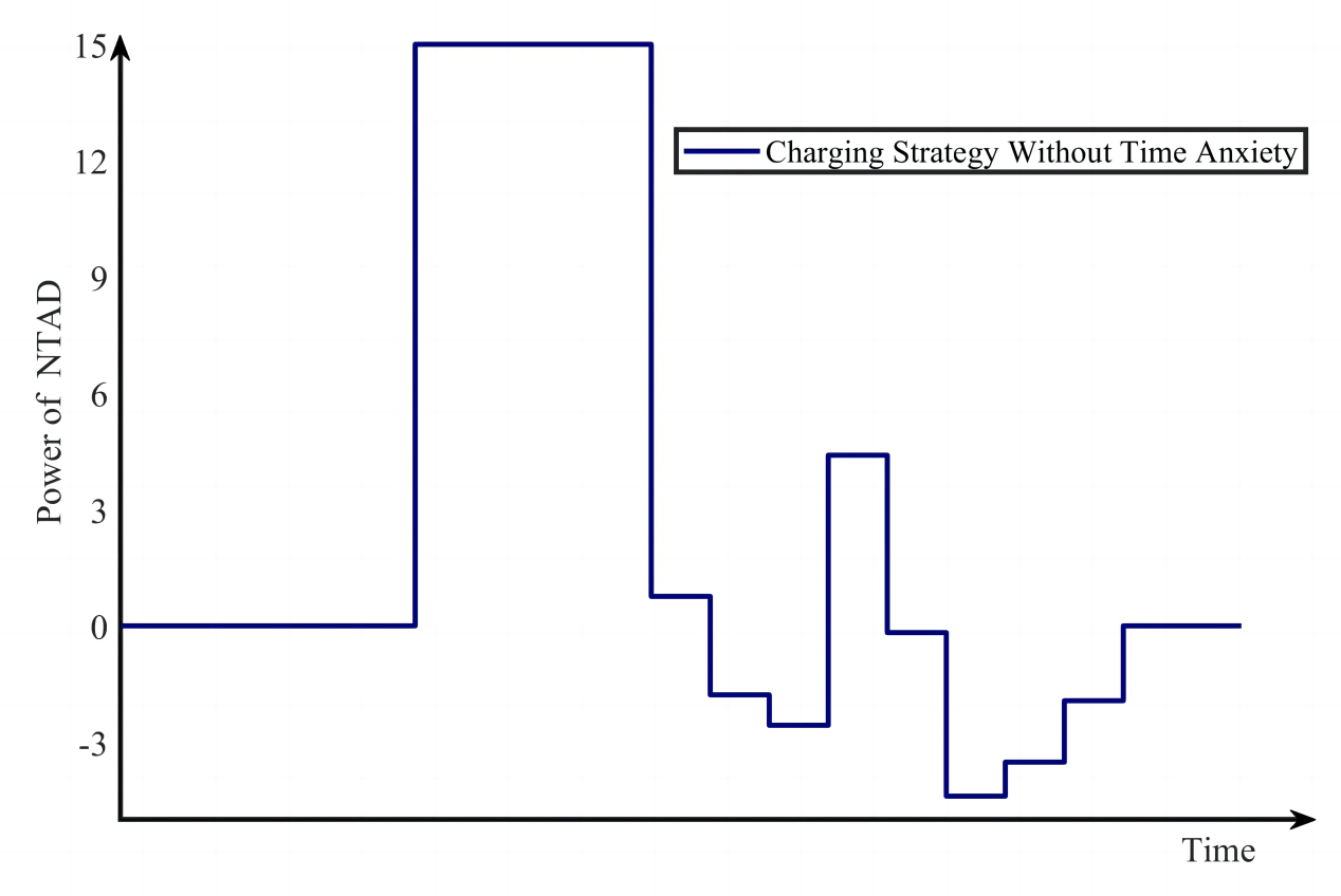
Non-time-anxious driver (NTAD): This type of driver reaches an anxious time directly after entering a state of peak anxiety (Figure 2).
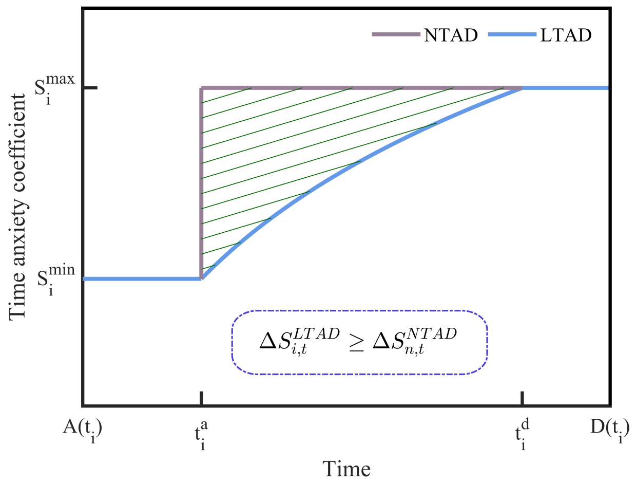
(2)
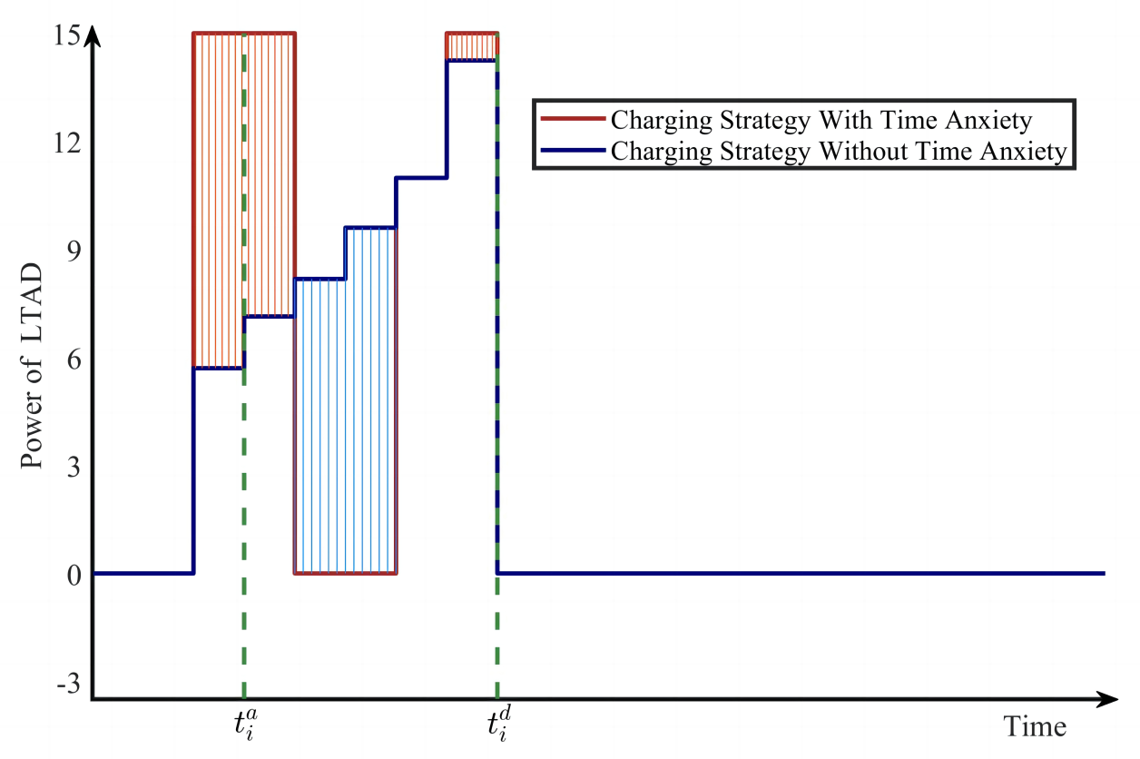
Less time-anxious driver (LTAD): This type of driver has anxiety values that rise quickly and then slowly after entering the anxious time. The rise is faster and then slower (Figure 3).
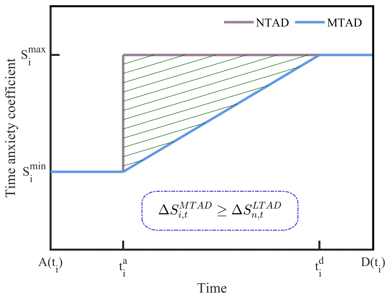
(3)
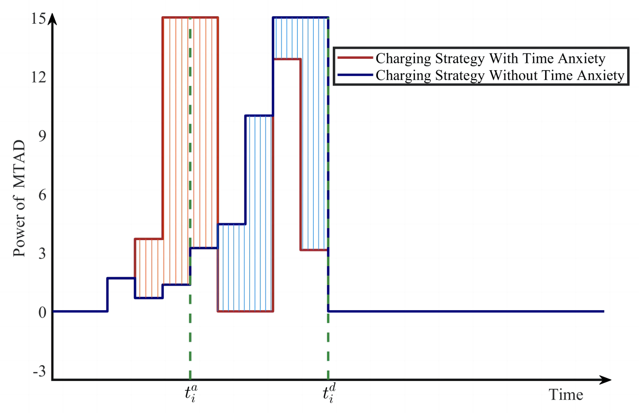
Mid-time-anxious driver (MTAD): This type of driver enters anxious time with anxiety values increasing at a uniform rate (Figure 4).
(4)
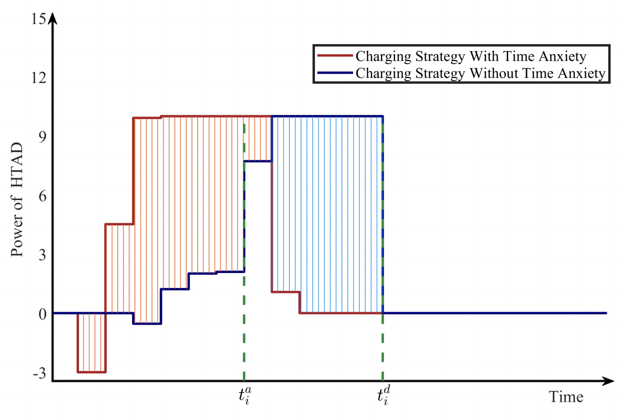
High-time-anxious driver (HTAD): This type of driver has anxiety values that rise slowly and then quickly after entering anxious time. The rise is slow and then fast (Figure 5).
Thus, we can obtain the following equation:
S i , t = S i , max , for NTAD ln V i , t ( e 1 ) + 1 × S i , max S i , min + S i , min , for LTAD V i , t S i , max S i , min + S i , min , for MTAD e V i , t 1 e 1 S i , max S i , min + S i , min , for HTAD
In Figure 2, Figure 3, Figure 4 and Figure 5, the value of S i , max S i , min indicates the PEV driver’s time anxiety, i.e., the depth of time anxiety. This indicates that the smaller the S i , min , the greater the time anxiety of the PEV driver. Furthermore, a greater time anxiety will increase the willingness of the PEV driver to meet the charging demand earlier and closer to the departure time, thus reducing the amount of time anxiety.
According to the preceding discussions, two factors will influence PEV drivers’ time anxiety. The intensity of time anxiety is the first, and the curve’s shape is the second. To represent the effect of curve shape, the curve shapes of the four different behavior types regarding time anxiety are shown in Figure 2, Figure 3, Figure 4 and Figure 5. We chose NATD as the reference, i.e., we chose S i , max as the reference value. The difference between this and the impact of time anxiety caused by the suggested behavior is referred to as the impact difference. For example, Δ S i , t LTAD = S i , t N A T D S i , t LTAD is defined as the impact difference of the LTAD behavior. Therefore, the following inequality (12) holds in Figure 2, Figure 3, Figure 4 and Figure 5:
Δ S i , t NTAD Δ S i , t LTAD Δ S i , t MTAD Δ S i , t HTAD

3. Distributed Charging Strategy

In this section, we propose a distributed reflected forward–backward splitting method to find a GNE of the function (8). Then, for the optimal response of each PEV driver, a distributed charging strategy is proposed. We assume that all PEVs in the SCS are selfish and each PEV is only allowed information about local problem data. Centralized control methods are typically unavailable in this situation.

3.1. Game Model

As the PEV charging and discharging problem is a generalized Nash equilibrium [24], we consider a group of agents I = { 1 , , N } that seek a GNE of the aggregative game with globally shared affine constraints and the gradient condition of KKT necessary optimality conditions can be then given by (13):
x i f i x i , σ ( x ) = d + N σ ( x ) + x i S i α + 1 T S i β
Assumption 1. 
For each i I , the function in (12) is differentiable and convex, and Ω R n is a closed convex set.
We define R m as m-dimensional Euclidean space and each agent i chooses its local decision x i Ω i R n . We call x = col x 1 , , x N = col x i i I Ω R N n the decision profile, i.e., the stacked vector i = 1 N Ω i = Ω . The aim of each agent i is to optimize its objective function, f i x i , σ ( x ) : Ω R , within its feasible decision set. Note that f i x i , σ ( x ) is nonlinearly coupled to the decisions of the other agents, but may not be explicitly coupled to the decisions of all other agents. We denote
X : = x i Ω i i = 1 N A i x i i = 1 N b i
where A i R m × n , b i R m are local data from agent i. Thus, we can obtain the following formula:
min x i f i x i , σ ( x ) s . t . i = 1 N A i x i i = 1 N b i
Furthermore, by considering games with affine sharing constraints A x b , and supposing x as a GNE of game (12), the optimal solution to the following convex optimization problem is defined as
min x i f i x i , σ ( x ) s . t . x i Ω i , A i x i b j i , j I A j x j
where b = i = 1 N b i R m . The set Ω i denotes the local decision set of agent i and the matrix A i defines how agent i is involved in the coupling constraint. However, the constraints of Equation (5) are clearly different from those of Equation (16). Therefore, the matrix A i and vector b i are then divided into two submatrices, H i and W i , and subvectors, P i and Q i . We define these as follows:
W i = 0 ( i 1 ) T × T E 0 ( N i ) T × T 0 ( i 1 ) T × T E 0 ( N i ) T × T I , P i = 0 ( i 1 ) R i 0 ( N i )
Q i = 0 ( i 1 ) T π i 1 π i min 1 T 0 ( i 1 ) T 0 ( i 1 ) T π i max π i 1 1 T 0 ( i 1 ) T C max N 1 T , H i = 0 ( i 1 ) × T 1 1 × T 0 ( N i ) × T
where 0 T represents the zero vector of T dimension, I represents the unit matrix and E = 1 1 1 · · · · · · · · · 1 1 · · · 1 R T × T . By definition, the constraints i = 1 N W i x i i = 1 N Q i , i = 1 N H i x i = i = 1 N P i are satisfied. Then, the constraints in Equation (5) are satisfied. Note that i = 1 N H i x i = i = 1 N P i is an equation constraint, while Equation (16) contains only the inequality constraint. Therefore, we represent this Equation constraint using two inequality constraints, satisfying both i = 1 N H i x i i = 1 N P i and i = 1 N H i x i i = 1 N P i . If using this approach, we need to rewrite A i = W i H i H i and b i = Q i P i P i , and the constraints in Equation (5) are converted into the constraints in Equation (16).
Assumption. 2 
For each i I , and for each ξ E , the function f i ( x i , σ ( x ) , ξ ) is Lipschitz continuous, convex, and continuously differentiable. For σ ( x ) , the Lipschitz constant ( σ ( x ) , ξ ) is integrable in ξ.
Among all possible generalized Nash equilibria, we are concerned with those solution sets that correspond to the set of solutions to an appropriate variational inequality. For this purpose, let us define the (pseudo) gradient mapping as
F ( x ) = col E x i f i x i , σ ( x ) , ξ i i I
We define a local Lagrangian function for agent i as L ( x , z , λ ) = F x , J x , x + Ω ( x ) + λ T ( A x b ) + R + N m ( λ ) + z T L λ λ , where λ i R + m is a dual variable associated with the coupling constraint. When x is an optimal solution to (16), the following Karush–Kuhn–Tucker (KKT) conditions are satisfied:
i I : 0 F x , J x + N Ω x + A T λ 0 = L λ λ 0 A x b N R + N m λ + L λ z
In order to ensure that all the preceding signs are + and facilitate the operation, the third formula becomes 0 A x + b + L λ λ + N R + N m λ L λ z . Since u ^ = M u is orthogonal to J u , there is no consistent vector in the space of u ^ to make L u u ^ = 0 when, and only when, u ^ = 0 . Meanwhile, we introduce L u to implement a distributed estimation. If we use I instead of L u , we need the central node to pass the average information. Based on this result, the extended KKT condition is as follows:
0 F x , J + u ^ + N Ω x + A T λ 0 = c L u u ^ 0 = L λ λ 0 A x + b + L λ λ + N R + N m λ L λ z

3.2. Distributed Algorithm

We assume that each driver only knows their local data, i.e., f i ( x i , σ ( x ) ) , Ω i , A i and b i , which contains their own private information. Meanwhile, the shared affine coupling constraints are decomposed such that each driver knows only one local block of the constraint matrix. Note that A i describes how agent i participates in the coupling constraints (shared global resources), which is also assumed to be privately known by driver i. The globally shared constraint A x b then couples the set of feasible decisions of the agents, but is not known to any agent. Next, we describe the preprocessing process leading to the distributed iteration proposed in the algorithm. In this, x i , k , u i , k , z i , k and λ i , k are the state variables of agent i at iteration k and τ i , v i , α i are fixed constant step-sizes for driver i. We define the weighted adjacency matrix W = w i , j i , j R N × N . The set of neighbors of PEV i is N i λ = j w i , j > 0 . We define the operators as follows:
A ¯ : x u z λ F x , J x + u c L u u 0 b + 0 0 0 L λ λ
B ¯ : x u z λ N Ω ( x ) 0 0 N R + Nm ( λ ) + 0 0 0 A T 0 0 0 0 0 0 0 L λ A 0 L λ 0 x u z λ
in which c R + . Meanwhile, the metric matrix Φ is defined as follows. Note that the matrix Φ is symmetric and positive definite, and the first term of Φ is the antisymmetric matrix in the operator B ¯ :
Φ = 0 0 0 A T 0 0 0 0 0 0 0 L λ A 0 L λ 0 + τ 1 0 0 0 0 0 0 0 0 0 v 1 0 0 0 0 α 1 + S C S 0 0 S κ 1 I 0 0 0 0 0 0 0 0 0 0 = τ 1 S C S 0 A T S κ 1 I 0 0 0 0 v 1 L λ A 0 L λ α 1
Through the RFB algorithm, we can obtain the following formula Φ v ¯ k + 1 + B ¯ v ¯ k + 1 = Φ v ¯ k A ¯ v k and v k + 1 = 2 v ¯ k + 1 v ¯ k , which is in the form of a distributed reflected forward–backward splitting method to find zeros of ( Φ 1 A + Φ 1 B ). We substitute the operators into Φ v ¯ k + 1 + B ¯ v ¯ k + 1 = Φ v ¯ k A ¯ v k , and then, through calculation, we can obtain the following equation:
N Ω x ¯ k + 1 + x ¯ k + 1 = x ¯ k + τ A T λ ¯ k F x k , J x k + u k c L k u k u ¯ k + 1 = u ¯ k κ c L k u k + M x ¯ k + 1 x ¯ k z ¯ k + 1 = z ¯ k v L λ λ ¯ k N R + N m λ ¯ k + 1 + λ ¯ k + 1 = λ ¯ k + α A 2 x ¯ k + 1 x ¯ k + L λ 2 z ¯ k + 1 z ¯ k b L λ λ k x k + 1 = 2 x ¯ k + 1 x ¯ k u k + 1 = 2 u ¯ k + 1 u ¯ k z k + 1 = 2 z ¯ k + 1 z ¯ k λ k + 1 = 2 λ ¯ k + 1 λ ¯ k
its initial condition is u ¯ 0 = x ¯ 0 and u 0 = x 0 .
Based on the above conclusions, the algorithm can find the GNE of the game, i.e., the strategy that finds the cost minimization for PEV i. Its convergence was proved in [18]. Meanwhile, by writing the above algorithm in distributed form, we can obtain the following Algorithm 1:
Algorithm 1: Distributed charging strategy with reflected forward-backward algorithm.
1:
Initialization: S i , min = S i , max = S , x i Ω i , u i R n , λ i R m and z i R m
2:
Task: slove (16)
3:
For k = 1 : k max
4:
        For  i = 1 : N
5:
(1)Receives x i , k for j N i f , u j , k , z j , k and λ j , k for j N i λ  then updates
6:
x ¯ i , k + 1 = proj Ω i x ¯ i , k + τ i A i T λ ¯ i , k x i f i x i , k , u i , k c j = 1 N ω i j u i , k u j , k
7:
u ¯ i , k + 1 = u ¯ i , k c κ j = 1 N ω i j u i , k u j , k + x ¯ i , k + 1 x ¯ i , k
8:
z ¯ i , k + 1 = z ¯ i , k v i j = 1 N ω i j λ ¯ i , k λ ¯ j , k
9:
λ ¯ i , k + 1 = proj R + m ( λ ¯ i , k + α ¯ i A i ( 2 x ¯ i , k + 1 x ¯ i , k α ¯ i b i j = 1 N ω i j ( λ i , k λ j , k )
10:
+ α ¯ i j = 1 N ω i j 2 z ¯ i , k + 1 z ¯ j , k + 1 z ¯ i , k z ¯ j , k )
11:
(2)Receives x ¯ i , k , u ¯ i , k , z ¯ i , k , λ ¯ i , k then updates
12:
x i , k + 1 = 2 x ¯ i , k + 1 x ¯ i , k
13:
u i , k + 1 = 2 u ¯ i , k + 1 u ¯ i , k
14:
z i , k + 1 = 2 z ¯ i , k + 1 z ¯ i , k
15:
λ i , k + 1 = 2 λ ¯ i , k + 1 λ ¯ i , k
16:
        end
17:
end
18:
if t = t i a t i d x i , t > p i c then
19:
        S i , min = S i , min ε
20:
       Go back to step 3
21:
else
22:
       break
23:
end if
Step 3 can be explained as follows. We define a step-size ε and set a threshold value p i c for time-anxious drivers. Since the initialization S i , min = S i , max = S , i.e., all drivers are not time-anxious, the algorithm is executed once, and a Nash equilibrium is solved. Then, we determine whether the sum of charging capacity t = t i a t i d x i , t for PEV i at the time t [ t i a , t i d ] is greater than the threshold value p i c . If t = t i a t i d x ¯ i , t > p i c , let S i , min = S i , min ε . Then, the new S i , min can be substituted to solve the Nash equilibrium once more. Otherwise, it is straightforward to derive the Nash equilibrium solution.

4. Simulation and Numerical Results

In this section, the performance of the proposed algorithm with load constraints and time anxiety is evaluated by minimizing the charging cost for PEV i in the SCS. For further illustration, we consider the SCS with 10 PEVs in the residential area. We also investigated the charging power distribution under non-time-anxious and time-anxious conditions. The simulation configuration was set up as follows.

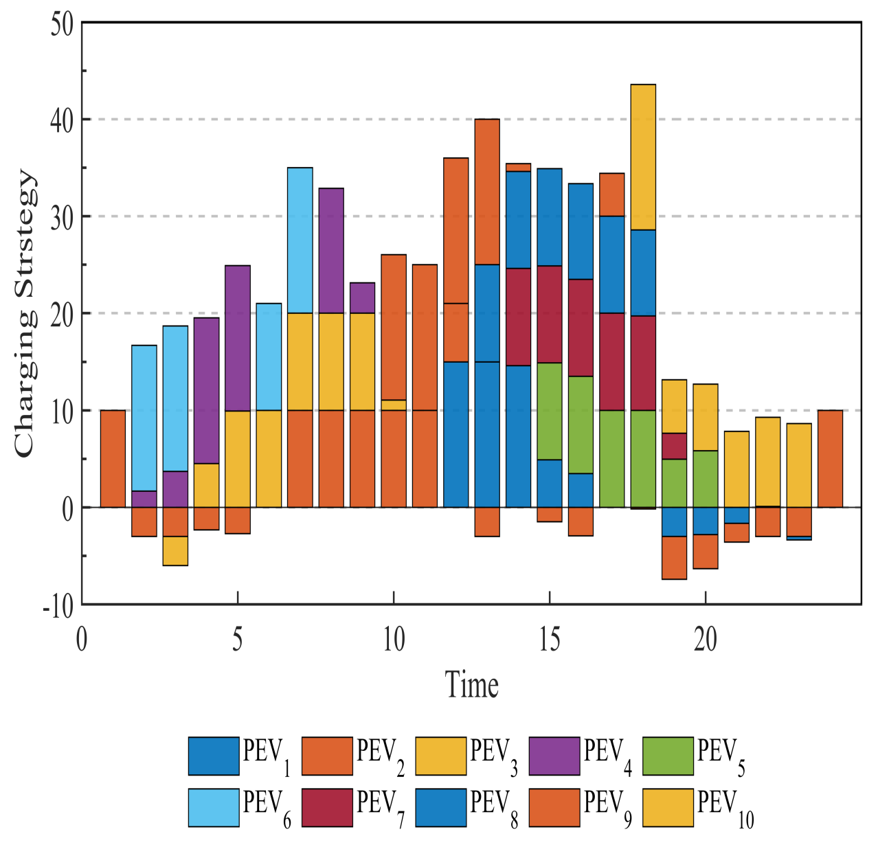
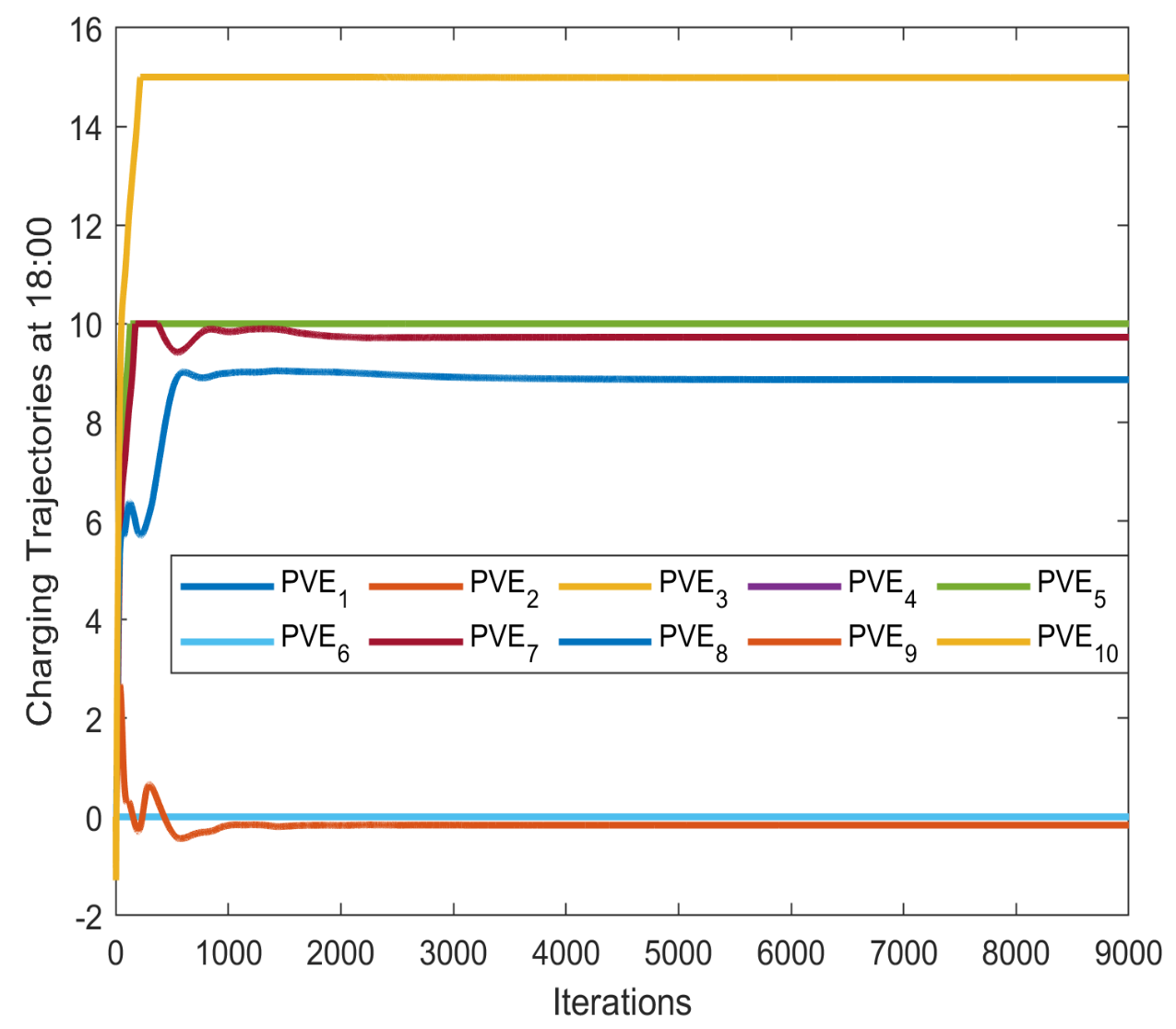
4.1. Overload Control for 10 PEVs

In this scenario, depending on the owner’s preferences and needs, 10 PEVs arrive at the SCS. The charging needs of each PEV were chosen between 50 and 60 KW, and the charging power was chosen between 10 and 15 KW/h. Table 1 lists the PEV parameters, arrival time (AT), and departure time (DT). Usually, the daily peak charging demand occurs from 12:00 to 17:00, when people go to the SCS to charge their PEVs. Therefore, we define α t = 0.3 $/kWh during peak hours (i.e., from 18:00 to 6:00), α t = 0.2 $/kWh during off-peak hours (i.e., other times), and the initial electricity price is β t = 0.3 $/kWh. We assume that the maximum power supplied by the SCS at time t is 130 KW, which is obtained from the value of [25].
As shown in Figure 6, the red dotted line shows the maximum capacity to support PEV charging at time t, i.e., L max = 130 KW. The green and purple solid lines denote the base load and the charging requirement load, respectively, for the 24 h. As shown in Figure 6, the SCS is severely overloaded at peak hours due to uncoordinated PEV charging, which may damage the SCS. Therefore, we present the overload control constraint in the framework of the game (16). After the overload control constraint, the load profile is shown in Figure 7. Compared with Figure 6, as the SCS in Figure 7 holds the charging capacity fixed at peak hours, the charging strategy shifts the excess charging capacity to free time, i.e., off-peak hours. The results show that the charging requirement load is always below the value of L max . Therefore, the strategy ensures the safety of the SCS.

4.2. Time Anxiety for PEVs

The simulation provides a further charging strategy considering load constraints. According to the settings in Table 1, the charging and discharging powers of each PEV are shown in Figure 8.
In these four pictures, the blue line indicates a charging strategy that does not consider time anxiety, while the red-brown line indicates a charging strategy that does consider time anxiety (note that the two are only different charging strategies; the amount that the PEV is charged does not change but is simply shifted). Figure 9 shows the NATD driver’s behavior in our simulation. From the discussion in Section 2.3, it follows that the driver has no time anxiety; therefore, the blue and red-brown lines overlap, and we use one of the blue lines to represent the PEV.
Figure 10 shows the LATD driver’s behavior in our simulation. From the previous discussion in Section 2.3, it follows that this driver will have some time anxiety, i.e., there may be a delay in the charging of the electric vehicle due to something that occurs during the time anxiety; therefore, a charging strategy that considers time anxiety will move some of the charging within the time interval [ t i a , t i d ] of time anxiety in the non-time anxious time interval, effectively avoiding the situation of missed EV charging due to unpredictable circumstances. This is represented in the graph by the transfer of the charge from anxious energy to shifted energy, which can be seen in Figure 10 as a reduction in the charge in the time anxious interval. The PEV driver is satisfied with the current charging method, as it is considered robust.
We simulated the behavior of the MATD driver, and, as can be seen in Figure 11, it shifted more of its charge to the rest of the time interval during the anxiety time interval than in Figure 10. The HATD driver, as can be seen in Figure 12, shifted more of its charge to the rest of the time interval during the anxious period than in Figure 11. This is because PEV drivers of various anxiety levels have a predefined threshold, which is lower if the drivers want to be more robust in response to uncertain events (e.g., HATD has the strongest anxiety). If the current anxiety energy exceeds the threshold, the PEV driver is dissatisfied with the current charge level, which would be insufficient to meet his or her charging needs in an uncertain event. Our algorithm is implemented in an iterative manner until the PEV driver succeeds in bringing his/her anxiety energy below its threshold, as indicated by the red-brown line. Our algorithm is iteratively implemented until the anxiety energy of the electric vehicle driver falls below a particular threshold.
The simulation of these four different driver behaviors leads to the same conclusion as discussed in Section 2.3: the greater the driver’s time anxiety, the greater that driver’s willingness to meet the charging demand earlier, i.e., more charging is transferred within the interval [ t i a , t i d ] of time anxiety.

4.3. Convergence Analysis

In this simulation, we provide an iterative process performed by all the PEVs at 18:00. PEVs do not need a central node to be able to bidirectionally communicate with all other PEVs. To preserve privacy, each PEV computes the corresponding decision in a distributed manner using its cost function, feasible set and coupling constraints. At each iteration k, the PEVs update their decisions and their estimates. The iterative process x k denotes the decision variable with PEV i; u k denotes the aggregated estimate, which includes the parameters that affect the electricity price; λ k is used to ensure that the constraints hold; z k is used as an auxiliary variable to ensure that λ k is consistent. As shown in Figure 13, the PEVs all converge to their optimal charging strategies during the iterative process. As a result, the proposed distributed RFB algorithm under the aggregative game can solve the charging problem in SCS proficiently.
In addition, we simulated the convergence accuracy of the RFB algorithm and the FB algorithm. Compared to the FB algorithm, the RFB algorithm converged to 10 7.1 and the FB algorithm converged to 10 3.6 after 9000 iterations under the same conditions shown in Figure 14. The effectiveness of the algorithm is demonstrated by the fact that it only takes 3000 iterations to converge to 10 3.6 using the RFB algorithm. The faster convergence indicates that all PEVs are solved to arrive at the optimal strategy faster.

5. Conclusions

In this paper, a new distributed charging and discharging strategy for PEVs, based on time anxiety and load constraints, was proposed in the framework of the aggregative game. Time anxiety was proposed to mitigate the effects of some uncertain events that may occur during charging. The load constraint was proposed to make the PEV charging more coordinated and protect the safety of the SCS. Detailed case studies were presented, showing that the charging strategy with time anxiety and load constraint considered is more reasonable and reduces the total cost. The distributed reflected forward–backward algorithm was designed to seek the generalized Nash equilibria of the game model. The proposed algorithm achieved optimal driver response in a theoretically fast, distributed manner and protected the driver’s privacy. The effectiveness of the proposed algorithm was verified by example simulations. In the future, we will focus on the aggregative game for charging stations.

Author Contributions

Conceptualization, T.K. and H.L.; methodology, T.K. and L.Z.; software, L.Z. and H.L.; validation, H.L.; formal analysis, T.K. and L.Z.; investigation, H.L.; resources, T.K. and H.L.; data curation, T.K. and L.Z.; writing—original draft preparation, T.K; writing—review and editing, H.L. and L.Z.; visualization, T.K. and H.L. and L.Z.; supervision, T.K. and H.L.; project administration, H.L.; funding acquisition, H.L. All authors have read and agreed to the published version of the manuscript.

Funding

The work described in this paper is supported in part by the National Natural Science Foundation of China (Grant No. 62173278) and in part by the Science and Technology Research Program of Chongqing Municipal Education Commission (Grant No. KJQN202100228).

Data Availability Statement

Not applicable.

Conflicts of Interest

The authors declare no conflict of interest.

References

  1. Poornesh, K.; Nivya, K.P.; Sireesha, K. A comparative study on electric vehicle and internal combustion engine vehicles. In Proceedings of the 2020 International Conference on Smart Electronics and Communication (ICOSEC), Trichy, India, 10–12 September 2020; IEEE: Piscataway, NJ, USA, 2020; pp. 1179–1183. [Google Scholar]
  2. Qian, K.; Zhou, C.; Allan, M.; Yuan, Y. Modeling of load demand due to EV battery charging in distribution systems. IEEE Trans. Power Syst. 2010, 26, 802–810. [Google Scholar] [CrossRef]
  3. Fischer, D.; Harbrecht, A.; Surmann, A.; McKenna, R. Electric vehicles’ impacts on residential electric local profiles—A stochastic modelling approach considering socio-economic, behavioural and spatial factors. Appl. Energy 2019, 233, 644–658. [Google Scholar] [CrossRef]
  4. Bilh, A.; Naik, K.; El-Shatshat, R. A novel online charging algorithm for electric vehicles under stochastic net-load. IEEE Trans. Smart Grid 2016, 9, 1787–1799. [Google Scholar] [CrossRef]
  5. Vatanparvar, K.; Faezi, S.; Burago, I.; Levorato, M.; Al Faruque, M.A. Extended Range Electric Vehicle With Driving Behavior Estimation in Energy Management. IEEE Trans. Smart Grid 2019, 10, 2959–2968. [Google Scholar] [CrossRef]
  6. Wang, C.; Zhou, Y.; Wu, J.; Wang, J.; Zhang, Y.; Wang, D. Robust-index method for household load scheduling considering uncertainties of customer behavior. IEEE Trans. Smart Grid 2015, 6, 1806–1818. [Google Scholar] [CrossRef]
  7. Alsabbagh, A.; Wu, B.; Ma, C. Distributed electric vehicles charging management considering time anxiety and customer behaviors. IEEE Trans. Ind. Inform. 2020, 17, 2422–2431. [Google Scholar] [CrossRef]
  8. Yan, Q.; Zhang, B.; Kezunovic, M. Optimized operational cost reduction for an EV charging station integrated with battery energy storage and PV generation. IEEE Trans. Smart Grid 2018, 10, 2096–2106. [Google Scholar] [CrossRef]
  9. Abdelaziz, M.M.A.; Shaaban, M.F.; Farag, H.E.; El-Saadany, E.F. A multistage centralized control scheme for islanded microgrids with PEVs. IEEE Trans. Sustain. Energy 2014, 5, 927–937. [Google Scholar] [CrossRef]
  10. Yao, L.; Lim, W.H.; Tsai, T.S. A Real-Time Charging Scheme for Demand Response in Electric Vehicle Parking Station. IEEE Trans. Smart Grid 2017, 8, 52–62. [Google Scholar] [CrossRef]
  11. Li, J.; Li, C.; Xu, Y.; Dong, Z.Y.; Wong, K.P.; Huang, T. Noncooperative Game-Based Distributed Charging Control for Plug-In Electric Vehicles in Distribution Networks. IEEE Trans. Ind. Inform. 2018, 14, 301–310. [Google Scholar] [CrossRef]
  12. Gan, L.; Topcu, U.; Low, S.H. Optimal decentralized protocol for electric vehicle charging. IEEE Trans. Power Syst. 2013, 28, 940–951. [Google Scholar] [CrossRef]
  13. Paccagnan, D.; Gentile, B.; Parise, F.; Kamgarpour, M.; Lygeros, J. Nash and wardrop equilibria in aggregative games with coupling constraints. IEEE Trans. Autom. Control 2018, 64, 1373–1388. [Google Scholar]
  14. Savadkoohi, S.J.S.; Kebriaei, H.; Aminifar, F. Aggregative Game for Charging Coordination of PEVs in a Network of Parking Lots. In Proceedings of the 2019 Smart Grid Conference (SGC), Tehran, Iran, 18–19 December 2019; IEEE: Piscataway, NJ, USA, 2019; pp. 1–6. [Google Scholar]
  15. Li, C.; Liu, C.; Deng, K.; Yu, X.; Huang, T. Data-Driven Charging Strategy of PEVs Under Transformer Aging Risk. IEEE Trans. Control. Syst. Technol. 2018, 26, 1386–1399. [Google Scholar] [CrossRef]
  16. Alsabbagh, A.; Yin, H.; Ma, C. Distributed Electric Vehicles Charging Management with Social Contribution Concept. IEEE Trans. Ind. Inform. 2020, 16, 3483–3492. [Google Scholar] [CrossRef]
  17. Gadjov, D.; Pavel, L. Distributed GNE seeking over networks in aggregative games with coupled constraints via forward-backward operator splitting. In Proceedings of the 2019 IEEE 58th Conference on Decision and Control (CDC), Nice, France, 11–13 December 2019; pp. 5020–5025. [Google Scholar]
  18. Cevher, V.; Vũ, B.C. A reflected forward-backward splitting method for monotone inclusions involving Lipschitzian operators. Set-Valued Var. Anal. 2021, 29, 163–174. [Google Scholar]
  19. Franci, B.; Staudigl, M.; Grammatico, S. Distributed forward-backward (half) forward algorithms for generalized Nash equilibrium seeking. In Proceedings of the 2020 European Control Conference (ECC), Saint Petersburg, Russia, 12–15 May 2020; pp. 1274–1279. [Google Scholar]
  20. Wan, Y.; Qin, J.; Li, F.; Yu, X.; Kang, Y. Game theoretic-based distributed charging strategy for PEVs in a smart charging station. IEEE Trans. Smart Grid 2020, 12, 538–547. [Google Scholar] [CrossRef]
  21. Jasim, A.M.; Jasim, B.H.; Neagu, B.C.; Alhasnawi, B.N. Efficient Optimization Algorithm-Based Demand-Side Management Program for Smart Grid Residential Load. Axioms 2023, 12, 33. [Google Scholar] [CrossRef]
  22. Liu, Y.; Deng, R.; Liang, H. A stochastic game approach for PEV charging station operation in smart grid. IEEE Trans. Ind. Informatics 2017, 14, 969–979. [Google Scholar] [CrossRef]
  23. Ma, Z.; Zou, S.; Liu, X. A distributed charging coordination for large-scale plug-in electric vehicles considering battery degradation cost. IEEE Trans. Control. Syst. Technol. 2015, 23, 2044–2052. [Google Scholar] [CrossRef]
  24. Ghavami, A.; Kar, K.; Gupta, A. Decentralized Charging of Plug-in Electric Vehicles With Distribution Feeder Overload Control. IEEE Trans. Autom. Control. 2016, 61, 3527–3532. [Google Scholar] [CrossRef]
  25. Pourakbari-Kasmaei, M.; Contreras, J.; Mantovani, J.R.S. A demand power factor-based approach for finding the maximum loading point. Electr. Power Syst. Res. 2017, 151, 283–295. [Google Scholar] [CrossRef] [Green Version]
Figure 1. Mechanism of interaction between SCS and PEV combined with the aggregative game.
Axioms 12 00186 g001
Figure 2. The time anxiety impact of NTAD.
Axioms 12 00186 g002
Figure 3. The time anxiety impact of LTAD.
Axioms 12 00186 g003
Figure 4. The time anxiety impact of MTAD.
Axioms 12 00186 g004
Figure 5. The time anxiety impact of HTAD.
Axioms 12 00186 g005
Figure 6. Charging strategies for 10 PEVs without overload control.
Axioms 12 00186 g006
Figure 7. Charging strategies for 10 PEVs with overload control.
Axioms 12 00186 g007
Figure 8. Charging capacity of 10 PEVs in a day.
Axioms 12 00186 g008
Figure 9. The time anxiety impact of NTAD.
Axioms 12 00186 g009
Figure 10. The time anxiety impact of LTAD.
Axioms 12 00186 g010
Figure 11. The time anxiety impact of MTAD.
Axioms 12 00186 g011
Figure 12. The time anxiety impact of HTAD.
Axioms 12 00186 g012
Figure 13. Charging trajectories of PEVs at 18:00.
Axioms 12 00186 g013
Figure 14. Convergence accuracy.
Axioms 12 00186 g014
Table 1. Constraint-related parameters.
PEV i π i 1 R i π i min π i max x i ¯ x i ̲ AT DT
1 7.5 5357515 15 1217
265658010 10 2214
38 52.5 57510 10 312
4 5.6 51.4 57015 15 210
5 6.7 5156510 10 1521
6 6.5 5657515 15 28
7 6.1 52.4 56510 10 420
895158010 10 1324
9 9.2 50.8 57015 15 1022
10 7.5 5357515 15 1824
Disclaimer/Publisher’s Note: The statements, opinions and data contained in all publications are solely those of the individual author(s) and contributor(s) and not of MDPI and/or the editor(s). MDPI and/or the editor(s) disclaim responsibility for any injury to people or property resulting from any ideas, methods, instructions or products referred to in the content.

