
A Fast Calculation Method for Sensitivity Analysis Using Matrix Decomposition Technique
Abstract
:1. Introduction
2. Sensitivity Reanalysis Using FDP
3. Numerical Examples
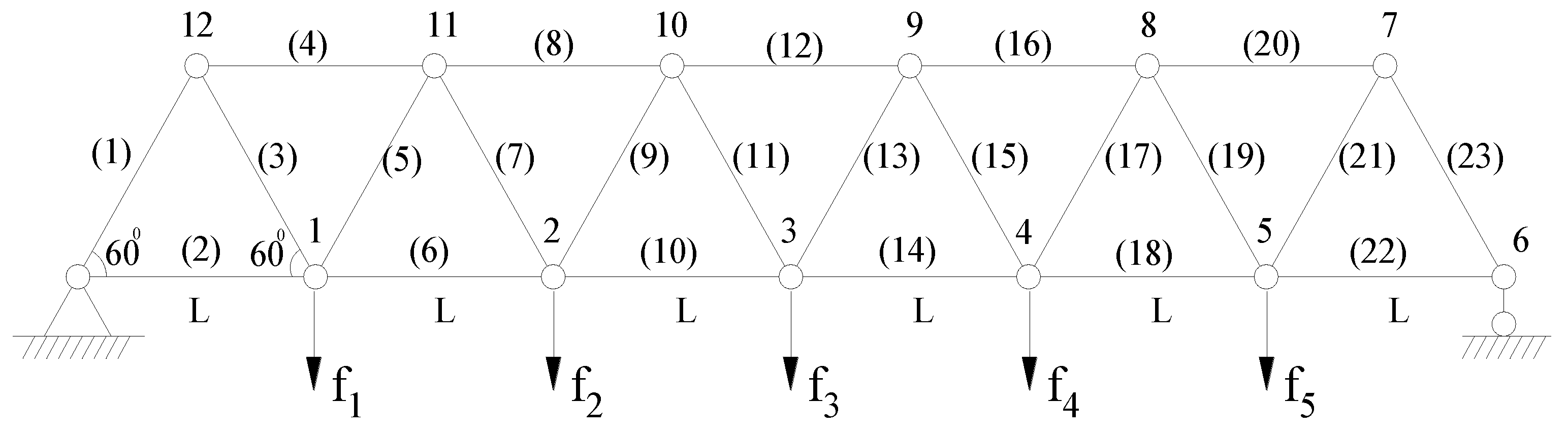
3.1. Statically Determinate Structure
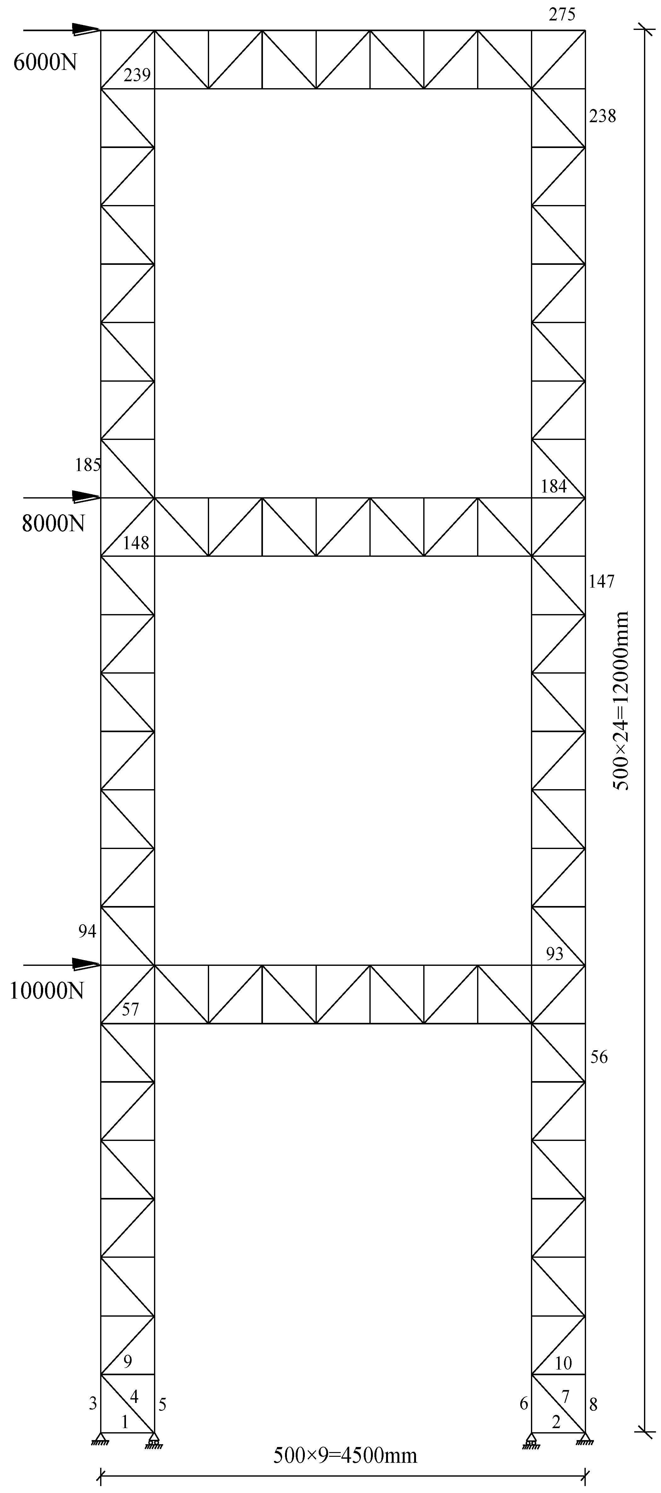
3.2. Statically Indeterminate Structure
4. Conclusions
Author Contributions
Funding
Data Availability Statement
Conflicts of Interest
References
- Lin, R.; Mottershead, J.; Ng, T. A state-of-the-art review on theory and engineering applications of eigenvalue and eigenvector derivatives. Mech. Syst. Signal Process. 2020, 138, 106536. [Google Scholar] [CrossRef]
- Yang, Q.; Peng, X. An Exact Method for Calculating the Eigenvector Sensitivities. Appl. Sci. 2020, 10, 2577. [Google Scholar] [CrossRef]
- Kirsch, U. Reanalysis of Structures; Springer: Dordrecht, The Netherlands, 2008. [Google Scholar]
- Yang, Q.W.; Peng, X. A highly efficient method for structural model reduction. Int. J. Numer. Methods Eng. 2023, 124, 513–533. [Google Scholar] [CrossRef]
- Cheikh, M.; Loredo, A. Static reanalysis of discrete elastic structures with reflexive inverse. Appl. Math. Model. 2002, 26, 877–891. [Google Scholar] [CrossRef]
- Chen, S.H.; Yang, Z.J. A universal method for structural static reanalysis of topological modifications. Int. J. Numer. Methods Eng. 2004, 61, 673–686. [Google Scholar] [CrossRef]
- Wu, B.; Li, Z. Static reanalysis of structures with added degrees of freedom. Commun. Numer. Methods Eng. 2006, 22, 269–281. [Google Scholar] [CrossRef]
- Zuo, W.; Yu, Z.; Zhao, S.; Zhang, W. A hybrid Fox and Kirsch’s reduced basis method for structural static reanalysis. Struct. Multidiscip. Optim. 2012, 46, 261–272. [Google Scholar] [CrossRef]
- Adelman, H.M.; Haftka, R.T. Sensitivity analysis of discrete structural systems. AIAA J. 1986, 24, 823–832. [Google Scholar] [CrossRef]
- Kirsch, U. Reanalysis and sensitivity reanalysis by combined approximations. Struct. Multidiscip. Optim. 2009, 40, 1–15. [Google Scholar] [CrossRef]
- Kirsch, U.; Bogomolni, M.; Sheinman, I. Efficient structural optimization using reanalysis and sensitivity reanalysis. Eng. Comput. 2007, 23, 229–239. [Google Scholar]
- Zuo, W.; Huang, K.; Bai, J.; Guo, G. Sensitivity reanalysis of vibration problem using combined approximations method. Struct. Multidiscip. Optim. 2017, 55, 1399–1405. [Google Scholar] [CrossRef]
- Chen, W.; Zuo, W. Component sensitivity analysis of conceptual vehicle body for lightweight design under static and dynamic stiffness demands. Int. J. Veh. Des. 2014, 66, 107–123. [Google Scholar] [CrossRef]
- Thomas, H.; Zhou, M. Issues of commercial optimization software development. Struct. Multidiscip. Optim. 2002, 23, 97–110. [Google Scholar] [CrossRef]
- Liu, J.; Wang, H. Fast sensitivity reanalysis methods assisted by Independent Coefficients and Indirect Factorization Updating strategies. Adv. Eng. Softw. 2018, 119, 93–102. [Google Scholar] [CrossRef]
- Zuo, W.; Bai, J.; Yu, J. Sensitivity reanalysis of static displacement using Taylor series expansion and combined approximate method. Struct. Multidiscip. Optim. 2016, 53, 953–959. [Google Scholar]
- Yang, Q. A new damage identification method based on structural flexibility disassembly. J. Vib. Control 2011, 17, 1000–1008. [Google Scholar] [CrossRef]
- Yang, Q.; Sun, B. Structural damage localization and quantification using static test data. Struct. Health Monit. 2011, 10, 381–389. [Google Scholar] [CrossRef]
- Yang, Q.W. Fast and Exact Algorithm for Structural Static Reanalysis Based on Flexibility Disassembly Perturbation. AIAA J. 2019, 57, 3599–3607. [Google Scholar] [CrossRef]
- Di, W.; Law, S. Eigen-parameter decomposition of element matrices for structural damage detection. Eng. Struct. 2007, 29, 519–528. [Google Scholar] [CrossRef]
- Akgün, M.A.; Garcelon, J.H.; Haftka, R.T. Fast exact linear and non-linear structural reanalysis and the Sherman-Morrison-Woodbury formulas. Int. J. Numer. Methods Eng. 2001, 50, 1587–1606. [Google Scholar] [CrossRef]
- Ren, J.; Zhang, Q. Structural Reanalysis Based on FRFs Using Sherman–Morrison–Woodbury Formula. Shock Vib. 2020, 3, 8212730. [Google Scholar]


| The Correction Coefficient αi | Scenario 1: Low-Rank Correction | Scenario 2: High-Rank Small Correction | Scenario 3: High-Rank Large Correction |
|---|---|---|---|
| α1 | 0 | 0.15 | 4.87 |
| α2 | 0 | 0.17 | 4.07 |
| α3 | 0 | −0.08 | −4.22 |
| α4 | 0 | 0.15 | 3.32 |
| α5 | 0.21 | 0.19 | −1.93 |
| α6 | 0 | −0.09 | −1.15 |
| α7 | 0 | −0.10 | −0.88 |
| α8 | 0 | 0.14 | −0.53 |
| α9 | 0.44 | −0.02 | −1.40 |
| α10 | 0 | 0.19 | −4.66 |
| α11 | 0 | −0.18 | 0.32 |
| α12 | 0 | 0.12 | 1.81 |
| α13 | 0 | 0.06 | −1.32 |
| α14 | −0.32 | −0.16 | 3.08 |
| α15 | 0 | 0.17 | −0.87 |
| α16 | 0 | −0.08 | 1.16 |
| α17 | 0 | 0.13 | 0.54 |
| α18 | 0 | 0.09 | −1.76 |
| α19 | 0 | −0.13 | −0.03 |
| α20 | 0 | −0.10 | 4.27 |
| α21 | 0 | 0.05 | 4.35 |
| α22 | 0 | 0.10 | −3.18 |
| α23 | 0 | 0.08 | 4.06 |
| DOF Number | Scenario 1: Low-Rank Correction | Scenario 2: High-Rank Small Correction | Scenario 3: High-Rank Large Correction | |||
|---|---|---|---|---|---|---|
| The Complete Analysis | The Proposed Reanalysis Algorithm | The Complete Analysis | The Proposed Reanalysis Algorithm | The Complete Analysis | The Proposed Reanalysis Algorithm | |
| 1 | 0.000 | 0.000 | 0.000 | 0.000 | 0.000 | 0.000 |
| 2 | 0.940 | 0.940 | 0.664 | 0.664 | 0.070 | 0.070 |
| 3 | 0.000 | 0.000 | 0.000 | 0.000 | 0.000 | 0.000 |
| 4 | 1.879 | 1.879 | 1.327 | 1.327 | 0.140 | 0.140 |
| 5 | −1.395 | −1.395 | −0.985 | −0.985 | −0.104 | −0.104 |
| 6 | 2.013 | 2.013 | 1.422 | 1.422 | 0.150 | 0.150 |
| 7 | −1.395 | −1.395 | −0.985 | −0.985 | −0.104 | −0.104 |
| 8 | 1.342 | 1.342 | 0.948 | 0.948 | 0.100 | 0.100 |
| 9 | −1.395 | −1.395 | −0.985 | −0.985 | −0.104 | −0.104 |
| 10 | 0.671 | 0.671 | 0.474 | 0.474 | 0.050 | 0.050 |
| 11 | −1.395 | −1.395 | −0.985 | −0.985 | −0.104 | −0.104 |
| 12 | −0.814 | −0.814 | −0.575 | −0.575 | −0.061 | −0.061 |
| 13 | 0.336 | 0.336 | 0.237 | 0.237 | 0.025 | 0.025 |
| 14 | −0.814 | −0.814 | −0.575 | −0.575 | −0.061 | −0.061 |
| 15 | 1.007 | 1.007 | 0.711 | 0.711 | 0.075 | 0.075 |
| 16 | −0.814 | −0.814 | −0.575 | −0.575 | −0.061 | −0.061 |
| 17 | 1.678 | 1.678 | 1.185 | 1.185 | 0.125 | 0.125 |
| 18 | −0.814 | −0.814 | −0.575 | −0.575 | −0.061 | −0.061 |
| 19 | 2.349 | 2.349 | 1.659 | 1.659 | 0.175 | 0.175 |
| 20 | −0.814 | −0.814 | −0.575 | −0.575 | −0.061 | −0.061 |
| 21 | 1.409 | 1.409 | 0.995 | 0.995 | 0.105 | 0.105 |
| 22 | −0.814 | −0.814 | −0.575 | −0.575 | −0.061 | −0.061 |
| 23 | 0.470 | 0.470 | 0.332 | 0.332 | 0.035 | 0.035 |
| DOF Number | Scenario 1: Low-Rank Correction | Scenario 2: High-Rank Small Correction | Scenario 3: High-Rank Large Correction | |||
|---|---|---|---|---|---|---|
| The Complete Analysis | The Proposed Reanalysis Algorithm | The Complete Analysis | The Proposed Reanalysis Algorithm | The Complete Analysis | The Proposed Reanalysis Algorithm | |
| 1 | 0.000 | 0.000 | 0.000 | 0.000 | 0.000 | 0.000 |
| 2 | −1.879 | −1.879 | −1.115 | −1.115 | 0.038 | 0.038 |
| 3 | 0.000 | 0.000 | 0.000 | 0.000 | 0.000 | 0.000 |
| 4 | −3.758 | −3.758 | −2.230 | −2.230 | 0.077 | 0.077 |
| 5 | 2.790 | 2.790 | 1.656 | 1.656 | −0.057 | −0.057 |
| 6 | −4.027 | −4.027 | −2.390 | −2.390 | 0.082 | 0.082 |
| 7 | 2.790 | 2.790 | 1.656 | 1.656 | −0.057 | −0.057 |
| 8 | −2.685 | −2.685 | −1.593 | −1.593 | 0.055 | 0.055 |
| 9 | 2.790 | 2.790 | 1.656 | 1.656 | −0.057 | −0.057 |
| 10 | −1.342 | −1.342 | −0.797 | −0.797 | 0.027 | 0.027 |
| 11 | 2.790 | 2.790 | 1.656 | 1.656 | −0.057 | −0.057 |
| 12 | 1.627 | 1.627 | 0.966 | 0.966 | −0.033 | −0.033 |
| 13 | −0.671 | −0.671 | −0.398 | −0.398 | 0.014 | 0.014 |
| 14 | 1.627 | 1.627 | 0.966 | 0.966 | −0.033 | −0.033 |
| 15 | −2.013 | −2.013 | −1.195 | −1.195 | 0.041 | 0.041 |
| 16 | 1.627 | 1.627 | 0.966 | 0.966 | −0.033 | −0.033 |
| 17 | −3.356 | −3.356 | −1.991 | −1.991 | 0.068 | 0.068 |
| 18 | 1.627 | 1.627 | 0.966 | 0.966 | −0.033 | −0.033 |
| 19 | −4.698 | −4.698 | −2.788 | −2.788 | 0.096 | 0.096 |
| 20 | 1.627 | 1.627 | 0.966 | 0.966 | −0.033 | −0.033 |
| 21 | −2.819 | −2.819 | −1.673 | −1.673 | 0.057 | 0.057 |
| 22 | 1.627 | 1.627 | 0.966 | 0.966 | −0.033 | −0.033 |
| 23 | −0.940 | −0.940 | −0.558 | −0.558 | 0.019 | 0.019 |
| Type of Correction | Modified Bars | is the Bar Number, |
|---|---|---|
| Type 1 | Bars 1~10 as shown in Figure 2 | |
| Type 2 | Bars 1~93 of the first story as shown in Figure 2 | |
| Type 3 | All bars (1~275) in Figure 2 | First story: Second story: Third story: |
| Type of Modification | The Complete Analysis | CA Method | Zuo’s Method | The Proposed Method |
|---|---|---|---|---|
| Type 1 (10 elements are revised) | = 0.262 s | = 0.166 s | = 0.161 s | = 0.083 s |
| = 36.6% | = 38.5% | = 68.3% | ||
| = 3.0% | = 50.0% | |||
| = 48.4% | ||||
| Type 2 (93 elements are revised) | = 0.254 s | = 0.191 s | = 0.174 s | = 0.097 s |
| = 24.8% | = 31.5% | = 61.8% | ||
| = 8.9% | = 49.2% | |||
| = 44.3% | ||||
| Type 3 (all elements are revised) | = 0.292 s | = 0.232 s | = 0.217 s | = 0.140 s |
| = 20.5% | = 25.7% | = 52.1% | ||
| = 6.5% | = 39.7% | |||
| = 35.5% |
| DOF Number | The Complete Analysis | CA Method | Zuo’s Method | The Proposed Method | ||||
|---|---|---|---|---|---|---|---|---|
| 10 | 1.659 | 1.518 | 1.657 | 1.516 | 1.663 | 1.531 | 1.659 | 1.518 |
| 11 | −0.551 | −0.496 | −0.551 | −0.495 | −0.552 | −0.500 | −0.551 | −0.496 |
| 12 | −0.187 | −0.169 | −0.187 | −0.169 | −0.188 | −0.171 | −0.187 | −0.169 |
| 13 | −0.551 | −0.496 | −0.551 | −0.495 | −0.552 | −0.500 | −0.551 | −0.496 |
| 14 | 0.169 | 0.154 | 0.168 | 0.154 | 0.169 | 0.155 | 0.169 | 0.154 |
| 15 | −0.979 | −0.908 | −0.979 | −0.909 | −0.981 | −0.915 | −0.979 | −0.908 |
| 16 | 0.344 | 0.310 | 0.344 | 0.309 | 0.345 | 0.313 | 0.344 | 0.310 |
| 17 | −0.979 | −0.908 | −0.979 | −0.909 | −0.981 | −0.915 | −0.979 | −0.908 |
| 18 | 1.492 | 1.364 | 1.491 | 1.362 | 1.496 | 1.376 | 1.492 | 1.364 |
| 19 | −1.047 | −0.949 | −1.046 | −0.948 | −1.049 | −0.957 | −1.047 | −0.949 |
| 20 | −0.260 | −0.237 | −0.260 | −0.237 | −0.260 | −0.239 | −0.260 | −0.237 |
| 21 | −1.047 | −0.949 | −1.046 | −0.948 | −1.049 | −0.957 | −1.047 | −0.949 |
| DOF Number | The Complete Analysis | CA Method | Zuo’s Method | The Proposed Method | ||||
|---|---|---|---|---|---|---|---|---|
| 10 | 0.837 | 0.622 | 0.835 | 0.619 | 0.971 | 0.813 | 0.837 | 0.622 |
| 11 | −0.244 | −0.171 | −0.240 | −0.165 | −0.283 | −0.224 | −0.244 | −0.171 |
| 12 | −0.087 | −0.062 | −0.086 | −0.061 | −0.101 | −0.081 | −0.087 | −0.062 |
| 13 | −0.244 | −0.171 | −0.240 | −0.165 | −0.283 | −0.224 | −0.244 | −0.171 |
| 14 | 0.083 | 0.060 | 0.084 | 0.062 | 0.096 | 0.079 | 0.083 | 0.060 |
| 15 | −0.540 | −0.413 | −0.563 | −0.447 | −0.626 | −0.540 | −0.540 | −0.413 |
| 16 | 0.155 | 0.110 | 0.143 | 0.093 | 0.180 | 0.144 | 0.155 | 0.110 |
| 17 | −0.540 | −0.413 | −0.563 | −0.447 | −0.626 | −0.540 | −0.540 | −0.413 |
| 18 | 0.747 | 0.553 | 0.742 | 0.547 | 0.866 | 0.723 | 0.747 | 0.553 |
| 19 | −0.492 | −0.355 | −0.490 | −0.352 | −0.571 | −0.464 | −0.492 | −0.355 |
| 20 | −0.128 | −0.094 | −0.129 | −0.095 | −0.149 | −0.123 | −0.128 | −0.094 |
| 21 | −0.492 | −0.355 | −0.490 | −0.352 | −0.571 | −0.464 | −0.492 | −0.355 |
| DOF Number | The Complete Analysis | CA Method | Zuo’s Method | The Proposed Method | ||||
|---|---|---|---|---|---|---|---|---|
| 10 | 1.738 | 1.660 | 1.736 | 1.658 | 1.739 | 1.664 | 1.738 | 1.660 |
| 11 | −0.587 | −0.561 | −0.587 | −0.560 | −0.588 | −0.562 | −0.587 | −0.561 |
| 12 | −0.198 | −0.190 | −0.198 | −0.189 | −0.198 | −0.190 | −0.198 | −0.190 |
| 13 | −0.587 | −0.561 | −0.587 | −0.560 | −0.588 | −0.562 | −0.587 | −0.561 |
| 14 | 0.177 | 0.170 | 0.177 | 0.169 | 0.177 | 0.170 | 0.177 | 0.170 |
| 15 | −1.012 | −0.967 | −1.010 | −0.966 | −1.012 | −0.969 | −1.012 | −0.967 |
| 16 | 0.366 | 0.350 | 0.366 | 0.349 | 0.367 | 0.350 | 0.366 | 0.350 |
| 17 | −1.012 | −0.967 | −1.010 | −0.966 | −1.012 | −0.969 | −1.012 | −0.967 |
| 18 | 1.565 | 1.496 | 1.563 | 1.494 | 1.566 | 1.498 | 1.565 | 1.496 |
| 19 | −1.107 | −1.058 | −1.106 | −1.056 | −1.108 | −1.060 | −1.107 | −1.058 |
| 20 | −0.273 | −0.261 | −0.273 | −0.261 | −0.273 | −0.262 | −0.273 | −0.261 |
| 21 | −1.107 | −1.058 | −1.106 | −1.056 | −1.108 | −1.060 | −1.107 | −1.058 |
| DOF Number | The Complete Analysis | CA Method | Zuo’s Method | The Proposed Method | ||||
|---|---|---|---|---|---|---|---|---|
| 10 | 1.193 | 0.996 | 1.181 | 0.976 | 1.242 | 1.079 | 1.193 | 0.996 |
| 11 | −0.403 | −0.336 | −0.399 | −0.329 | −0.420 | −0.364 | −0.403 | −0.336 |
| 12 | −0.137 | −0.114 | −0.136 | −0.113 | −0.142 | −0.124 | −0.137 | −0.114 |
| 13 | −0.403 | −0.336 | −0.399 | −0.329 | −0.420 | −0.364 | −0.403 | −0.336 |
| 14 | 0.122 | 0.102 | 0.121 | 0.100 | 0.128 | 0.111 | 0.122 | 0.102 |
| 15 | −0.698 | −0.584 | −0.692 | −0.574 | −0.727 | −0.633 | −0.698 | −0.584 |
| 16 | 0.250 | 0.208 | 0.247 | 0.203 | 0.260 | 0.225 | 0.250 | 0.208 |
| 17 | −0.698 | −0.584 | −0.692 | −0.574 | −0.727 | −0.633 | −0.698 | −0.584 |
| 18 | 1.075 | 0.898 | 1.065 | 0.880 | 1.120 | 0.973 | 1.075 | 0.898 |
| 19 | −0.761 | −0.635 | −0.753 | −0.623 | −0.792 | −0.688 | −0.761 | −0.635 |
| 20 | −0.188 | −0.157 | −0.187 | −0.155 | −0.196 | −0.171 | −0.188 | −0.157 |
| 21 | −0.761 | −0.635 | −0.753 | −0.623 | −0.792 | −0.688 | −0.761 | −0.635 |
| DOF Number | The Complete Analysis | CA Method | Zuo’s Method | The Proposed Method | ||||
|---|---|---|---|---|---|---|---|---|
| 10 | 1.736 | 1.656 | 1.734 | 1.655 | 1.737 | 1.660 | 1.736 | 1.656 |
| 11 | −0.587 | −0.560 | −0.586 | −0.559 | −0.587 | −0.561 | −0.587 | −0.560 |
| 12 | −0.198 | −0.189 | −0.198 | −0.189 | −0.198 | −0.190 | −0.198 | −0.189 |
| 13 | −0.587 | −0.560 | −0.586 | −0.559 | −0.587 | −0.561 | −0.587 | −0.560 |
| 14 | 0.177 | 0.169 | 0.177 | 0.169 | 0.177 | 0.169 | 0.177 | 0.169 |
| 15 | −1.010 | −0.964 | −1.009 | −0.963 | −1.011 | −0.966 | −1.010 | −0.964 |
| 16 | 0.366 | 0.349 | 0.366 | 0.349 | 0.366 | 0.350 | 0.366 | 0.349 |
| 17 | −1.010 | −0.964 | −1.009 | −0.963 | −1.011 | −0.966 | −1.010 | −0.964 |
| 18 | 1.563 | 1.492 | 1.562 | 1.490 | 1.564 | 1.495 | 1.563 | 1.492 |
| 19 | −1.106 | −1.055 | −1.105 | −1.054 | −1.106 | −1.058 | −1.106 | −1.055 |
| 20 | −0.273 | −0.260 | −0.272 | −0.260 | −0.273 | −0.261 | −0.273 | −0.260 |
| 21 | −1.106 | −1.055 | −1.105 | −1.054 | −1.106 | −1.058 | −1.106 | −1.055 |
| DOF Number | The Complete Analysis | CA Method | Zuo’s Method | The Proposed Method | ||||
|---|---|---|---|---|---|---|---|---|
| 10 | 1.181 | 0.981 | 1.173 | 0.969 | 1.234 | 1.071 | 1.181 | 0.981 |
| 11 | −0.399 | −0.332 | −0.397 | −0.328 | −0.417 | −0.362 | −0.399 | −0.332 |
| 12 | −0.135 | −0.112 | −0.134 | −0.111 | −0.141 | −0.123 | −0.135 | −0.112 |
| 13 | −0.399 | −0.332 | −0.397 | −0.328 | −0.417 | −0.362 | −0.399 | −0.332 |
| 14 | 0.121 | 0.101 | 0.120 | 0.099 | 0.126 | 0.110 | 0.121 | 0.101 |
| 15 | −0.689 | −0.573 | −0.685 | −0.567 | −0.720 | −0.626 | −0.689 | −0.573 |
| 16 | 0.248 | 0.206 | 0.246 | 0.203 | 0.259 | 0.224 | 0.248 | 0.206 |
| 17 | −0.689 | −0.573 | −0.685 | −0.567 | −0.720 | −0.626 | −0.689 | −0.573 |
| 18 | 1.064 | 0.884 | 1.057 | 0.874 | 1.111 | 0.965 | 1.064 | 0.884 |
| 19 | −0.753 | −0.626 | −0.749 | −0.619 | −0.787 | −0.683 | −0.753 | −0.626 |
| 20 | −0.186 | −0.155 | −0.185 | −0.153 | −0.194 | −0.169 | −0.186 | −0.155 |
| 21 | −0.753 | −0.626 | −0.749 | −0.619 | −0.787 | −0.683 | −0.753 | −0.626 |
Disclaimer/Publisher’s Note: The statements, opinions and data contained in all publications are solely those of the individual author(s) and contributor(s) and not of MDPI and/or the editor(s). MDPI and/or the editor(s) disclaim responsibility for any injury to people or property resulting from any ideas, methods, instructions or products referred to in the content. |
© 2023 by the authors. Licensee MDPI, Basel, Switzerland. This article is an open access article distributed under the terms and conditions of the Creative Commons Attribution (CC BY) license (https://creativecommons.org/licenses/by/4.0/).
Share and Cite
Yang, Q.; Peng, X. A Fast Calculation Method for Sensitivity Analysis Using Matrix Decomposition Technique. Axioms 2023, 12, 179. https://doi.org/10.3390/axioms12020179
Yang Q, Peng X. A Fast Calculation Method for Sensitivity Analysis Using Matrix Decomposition Technique. Axioms. 2023; 12(2):179. https://doi.org/10.3390/axioms12020179
Chicago/Turabian StyleYang, Qiuwei, and Xi Peng. 2023. "A Fast Calculation Method for Sensitivity Analysis Using Matrix Decomposition Technique" Axioms 12, no. 2: 179. https://doi.org/10.3390/axioms12020179