5.1. Selected Models
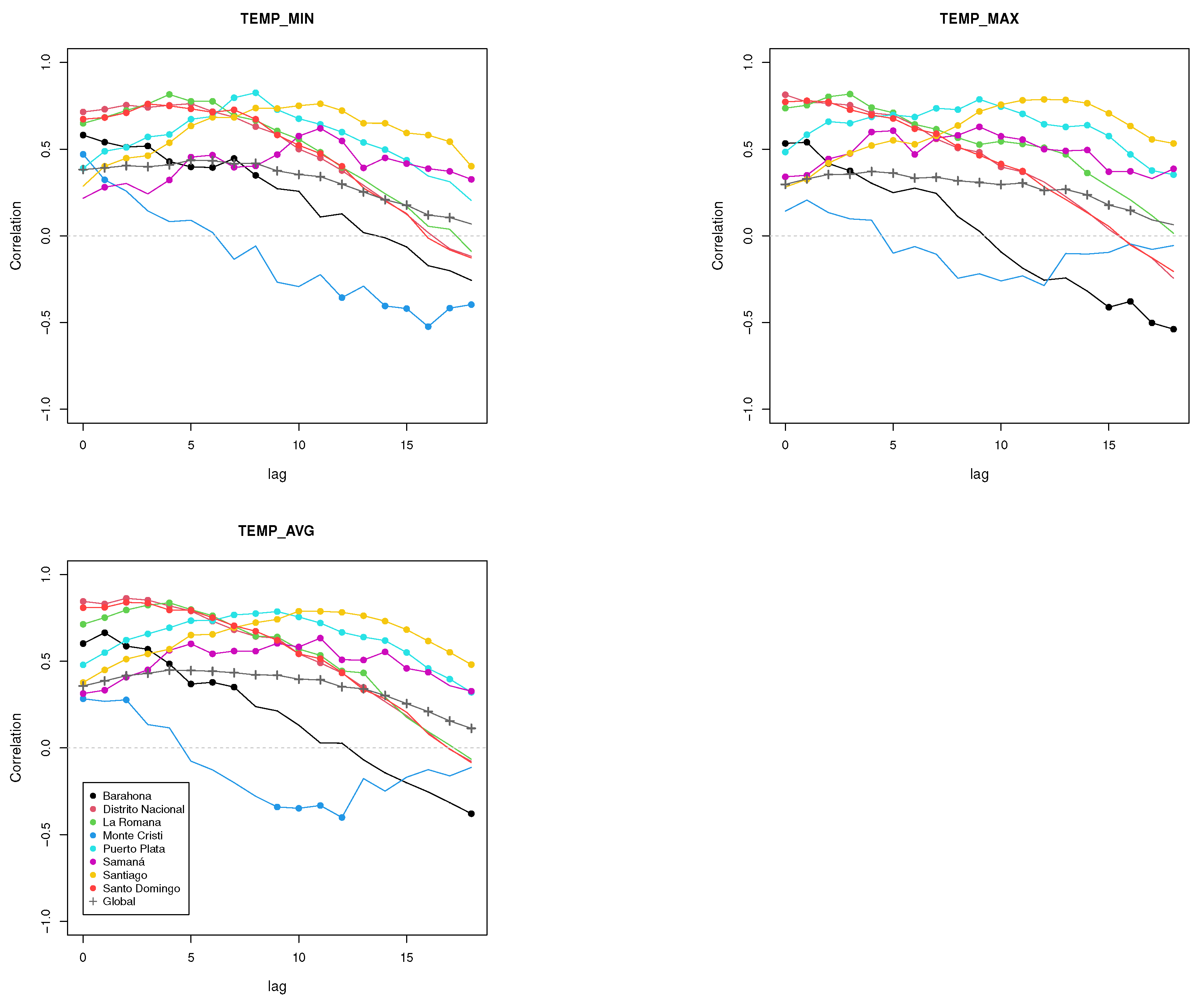
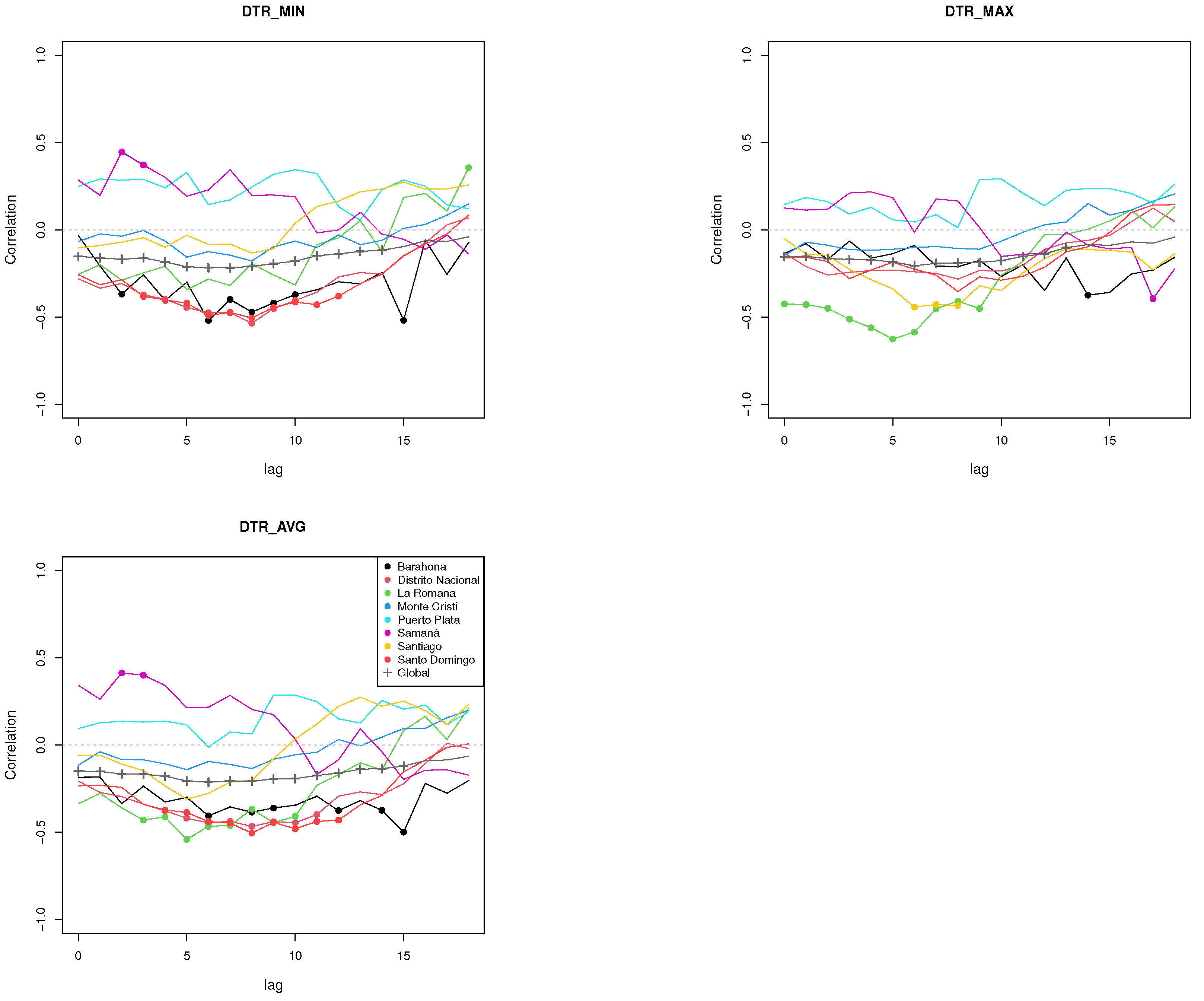
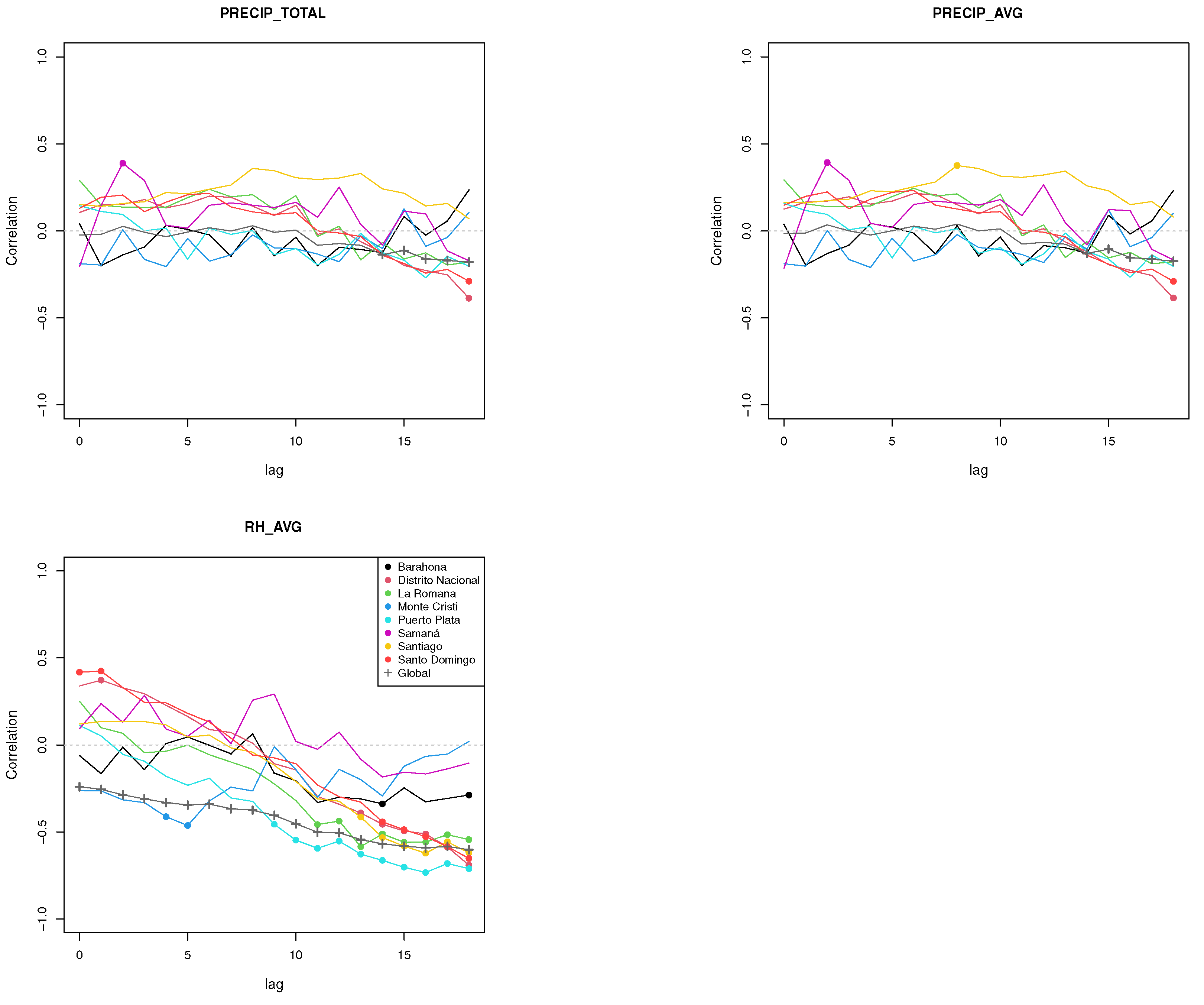
Based on the lags suggested by Criterion I-IV (
Section 4.5), twelve multiple gamma-GLMMs for estimating the adjusted incidence rate (Equation (
7)) in terms of meteorological regressors were constructed: models M01-M12 with lags of meteorological variables as indicated in
Table 4. For the construction of these models, we considered the variable Precip.avg as the precipitation regressor. For six of these models, the process of estimating the parameters was not convergent (i.e., the iteration process in the optimizer via the R-function
glmer was stopped without an optimum value for the objective function) as noted in the last column in
Table 4. Among the remaining six models, the lowest AIC was achieved by the model M12, which employs as explanatory variables the weekly average and minimum temperatures and average DTR with a lag of 5 weeks, the weekly maximum temperature with a lag of 4 weeks, and the average weekly precipitation with a lag of 2 weeks. M12 also included the maximum and minimum DTR with a lag of 5 weeks, but these variables were not significant to predictions.
In fact, the variable DTR.max was not a significant predictor in any of the previous models, so it was removed, and we replicated the procedure as before. With DTR.max removed, a total of eight models were developed, M13-M20 as indicated in
Table 4. Among the convergent models, the lowest AIC was achieved to the model M20, which included all of the same predictors as M12 excepting DTR.max.
For both models, M12 and M20, the same set of independent variables was obtained as statistically significant: Temp.avg, Temp.max, Temp.min, DTR.avg, DTR.min and Precip.avg with lag equals to 5, 4, 5, 5, 5, and 2 weeks, respectively. Finally, because the variable DTR.min (with lag = 5 weeks) is not statistically significantly in the model, it was removed at this stage to obtain the final model (M21 in
Table 4) which reached a slightly lower AIC value than the previous ones.
In this final model, temperature and DTR variables have larger lags. Therefore, this model could represent a long-term alarm based on both temperature and DTR conditions. Therefore, it will be called a longer-term model. Given this result, we aimed to next answer the question: could these same variables predict adjusted dengue incidence rate in a shorter time? Consequently, an extra model (M22 in
Table 4), called a shorter-term model, with all these variables with a delay of 2 weeks was analyzed. All variables with a delay of 2 weeks were significant predictors; however, the AIC for M22 was not lower than that of M21, indicating that it is not a better model overall.
We note that the procedure described above was replicated substituting the variable Precip.avg by Precip.total as a precipitation regressor. Under this condition, more nonconvergent models emerged, and slightly higher values of AIC were in general produced for the convergent homologous models (data not shown). We also note that when the random intercepts
are not included in the multiple model (
5) (i.e., where the approach GLM is used for modelling of the adjusted dengue incidence rate (Equation (
7)), substantially higher values of AIC would be obtained for the correspondent GLMs, namely AIC = 1923.7 and AIC = 1936.8) for the fitted longer-term model and shorter-term model, respectively, justifying the modelling of the dengue data set by GLMM than by GLM.
As indicated in
Table 4, in the longer-term model (M21), the weekly dengue incidence rate is described in of terms the average and the minimum values of the temperature both delayed by 5 weeks (Temp.avg5 and Temp.min5), the maximum value of the temperature delayed by 4 weeks (Temp.max4), and the average value of precipitation delayed by 2 weeks (Precip.avg2). In the
shorter-term model (M22), the weekly dengue incidence rate is described by effects of those five meteorological features all with a delay of 2 weeks (Temp.avg2, Temp.max2, Temp.min2, DTR.avg2, and Precip.avg2).
Formally, these two models are defined as follows,
and
respectively, for each province
, and meteorological conditions summarized in epidemiological week
of 2019. The variable Province
is assumed to be normally distributed with zero mean and constant variance
in the estimation process of the regressor coefficients in each model and represents the random effect specific (Y-intercept) to the
ith province.
5.2. Validation
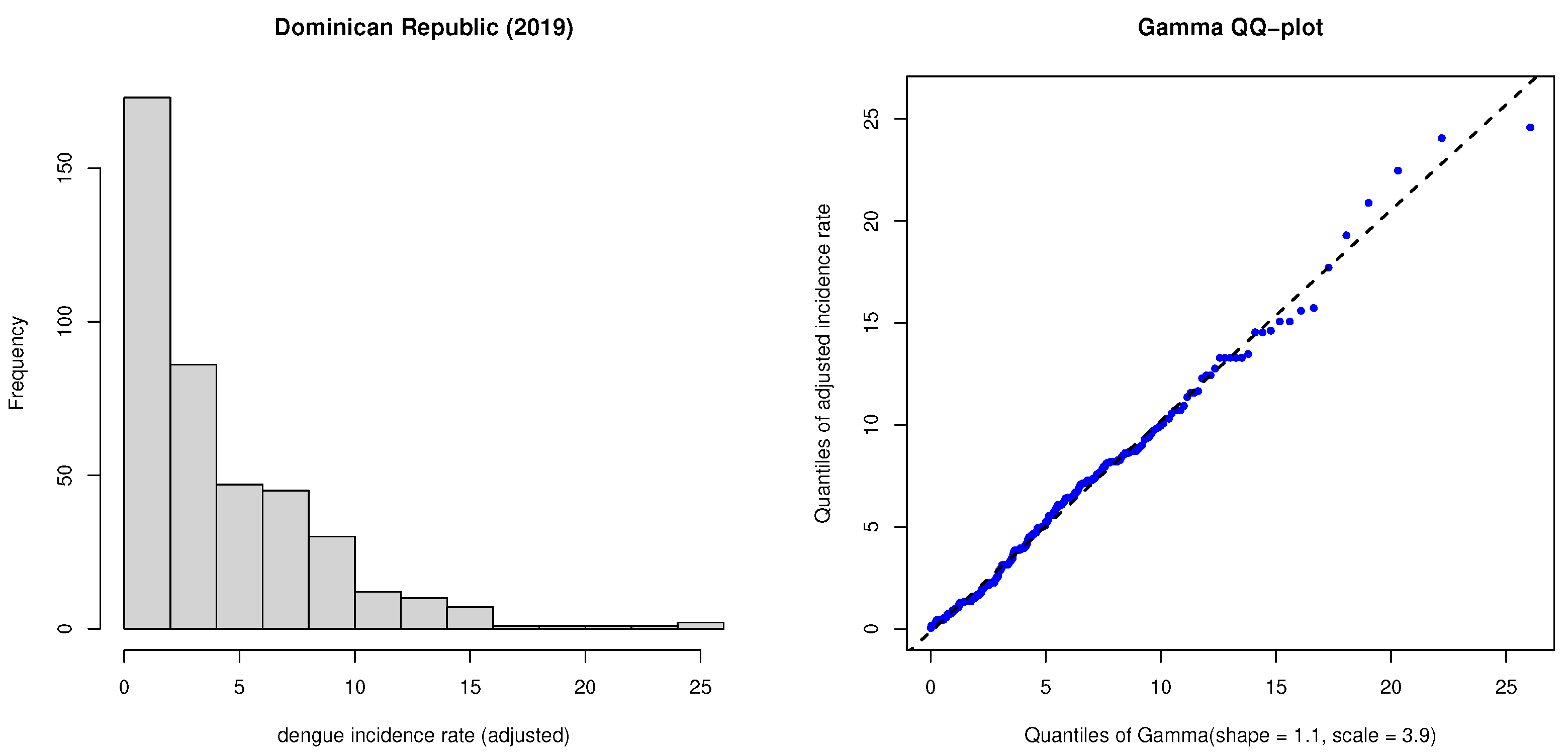
The histogram and the QQ-plot presented in
Figure 5 suggest that the empirical right-skewed distribution of the adjusted rates (Equation (
7)) for the set of the eight provinces is close to a gamma distribution (with
and
). There was no significant evidence that a gamma distribution did not provide an adequate fit (
V = 0.51294,
p-value = 0.7168).
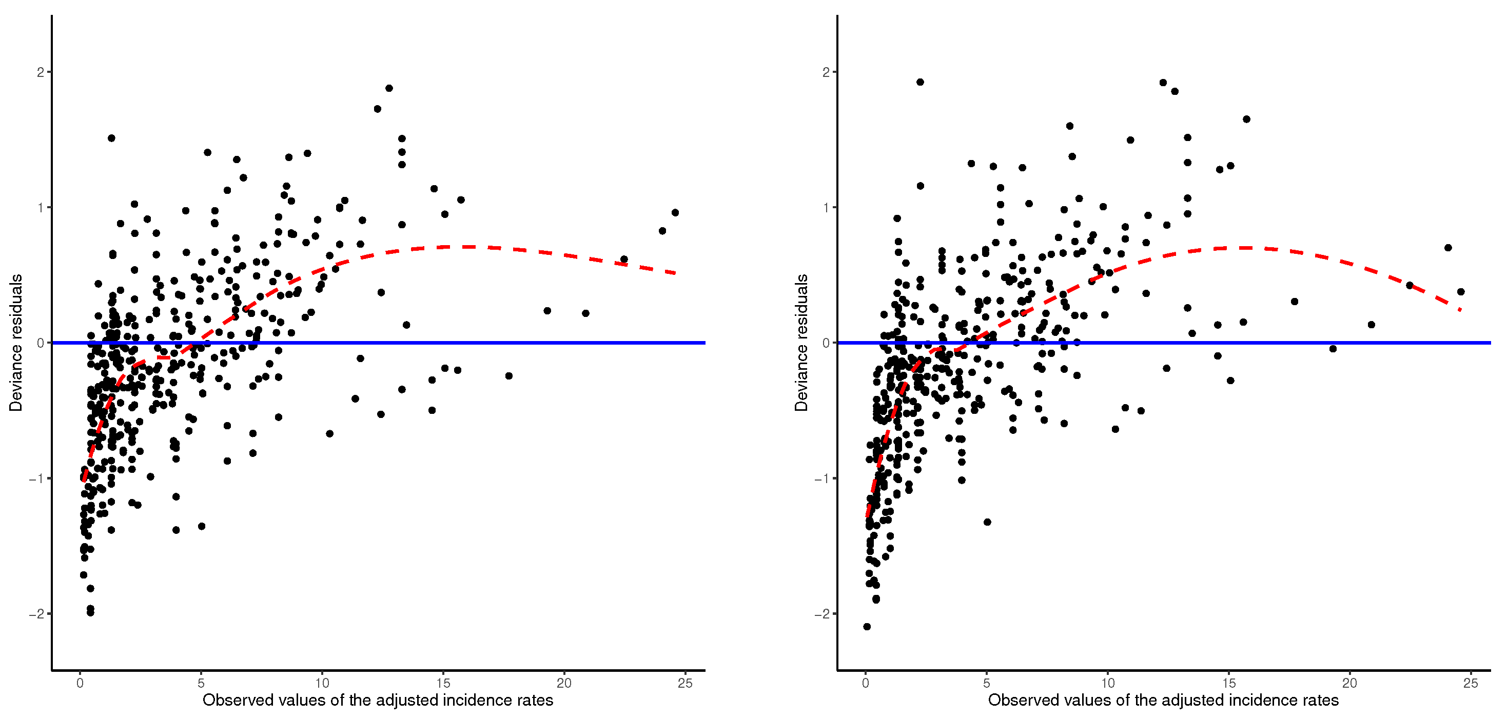
In
Figure 6, for both models, it is observed that almost all of the deviance residuals vary between −2 and 2 and there is a higher spread of points for higher observed values of the incidence rate (
7). When the observed incidence rate is close to zero, there are many negative residuals suggesting that both models tend to predict higher incidence rates than the observed rates. For higher observed values (e.g., for weekly incidence rate between approximately 6 and 15 per 100,000 inhabitants), both the smoothed average curves (red lines in the graphs) tend to increase, indicating that the values predicted by both models will be lower than the observed. Nevertheless, for situations with the highest incidence rates, the fitted curve is closer to zero in the shorter-term model. This suggests that meteorological conditions of temperature, DTR and precipitation of 2 weeks earlier tend to provide better predictions for dengue incidence when outbreaks are larger than than those predictions using longer delays.
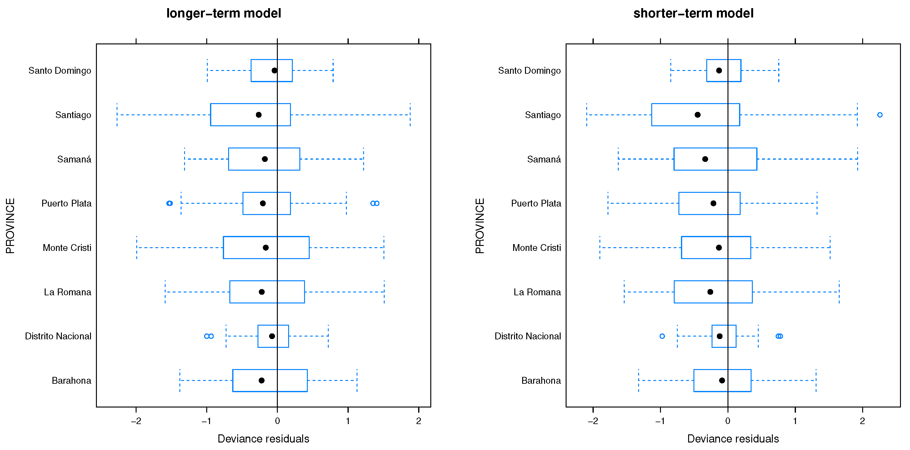
In
Figure 7, the comparative boxplots of the deviance residuals for the eight provinces show that (i) the deviance residuals only exceeds the interval [−2, 2] in Santiago, and only slightly; (ii) there are outliers, suggesting that there are a few weeks when the model estimates of the incidence rates could be atypical (in Distrito Nacional, Puerta Plata and Santiago); and (iii) the variability in two provinces, Santo Domingo and Distrito Nacional, seems to be lower than in other provinces. Although these results indicate the models do not always predict the true incidence rates in some weeks and some provinces, both the models fit relatively well to the data.
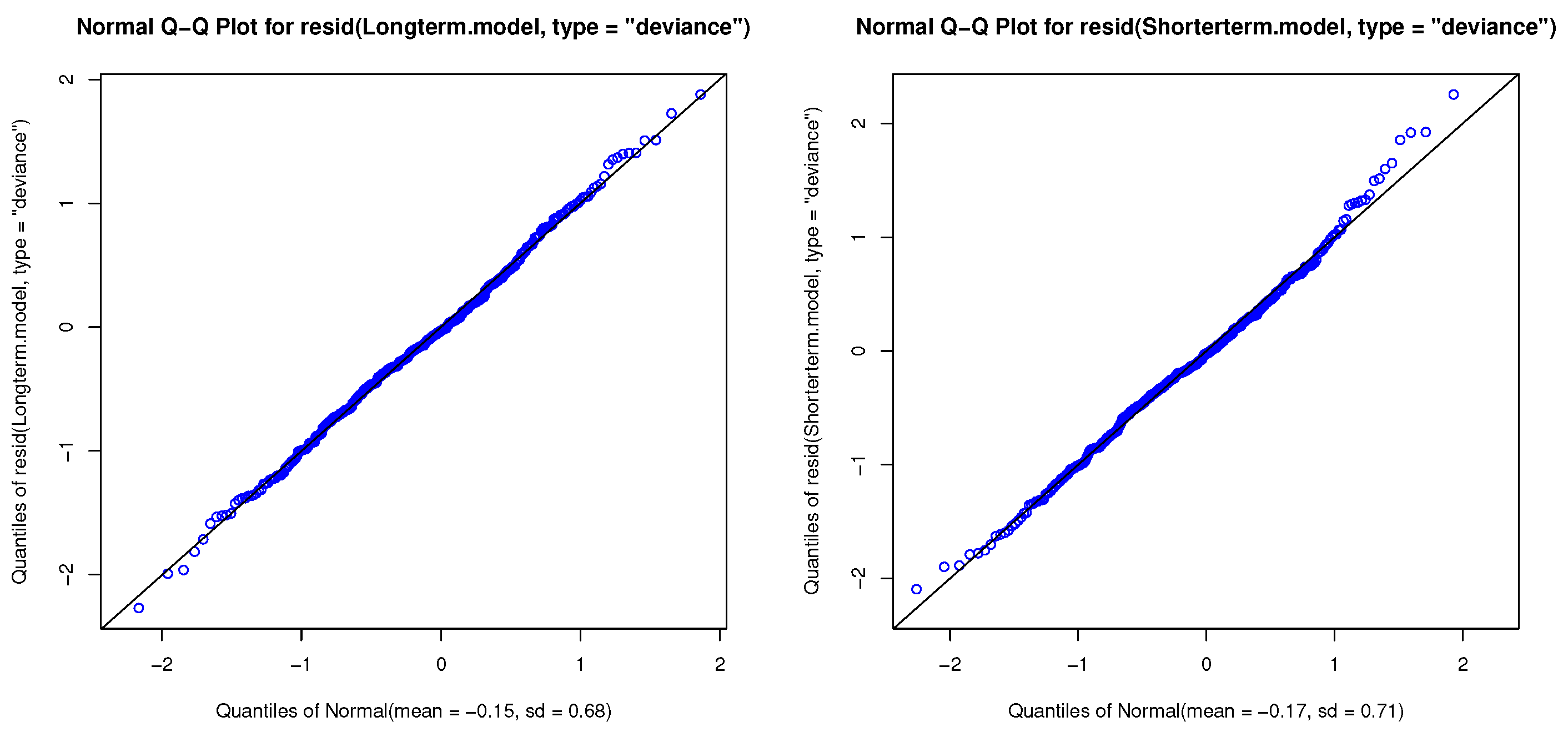
In
Figure 8, the good alignment of the points with the diagonal line in both the QQ-plots suggests a normal distribution to the deviance residuals for both models. From the Shapiro–Wilks test, there was no significant evidence that the distributions of deviance residuals of both models were nonnormal (
p-value = 0.818 for longer-term model and
p-value = 0.136 for the shorter-term model).
5.3. Interpretation
The estimates of the fixed effects and the effect variance of the two fitted models are displayed in
Table 5. Only a single covariate coefficient (Temp.max2 for the
shorter-term model) was not statistically significantly different from zero at a 5% significance level. Therefore, associations between each significant meteorological variable and the dengue incidence rate for the eight provinces of Dominican Republic can be then described assuming that the remaining variables are fixed. Variations in the daily average temperature (Temp.avg) have the greatest effect on the dependent variable (dengue incidence rate) with an increase of 1 °C leading to an increase in the dengue incidence rate by 52.4% (
) 2 weeks later and 44.4% (
) 5 weeks later. Although the same increase of the maximum temperature (Temp.max) increases the dengue incidence rate by 3.5% (
) 2 weeks later and 13% (
) 4 weeks later, the minimum temperature (Temp.min) reduces the rate of reported cases by 5.0% (
) 2 weeks later and 6.0% (
) 5 weeks later. If the average daily temperature range (DTR.avg) is 1 °C higher, then a decrease of 18.3% (
) and 11.5% (
) in dengue incidence rate is observed 5 and 2 weeks later, respectively. A 1-mm increase in the weekly average precipitation (Precip.avg) triggers an increase in the dengue incidence rate of 2.0% (
) and 4.5% (
) 2 weeks later for the longer-term and shorter-term models, respectively.
The variances of the random effects, , were estimated to be equal to 0.2363 and 0.2764 for the longer-term and shorter-term models, respectively. This result indicates slightly lower variability among the eight provinces for the Y-intercept of the fitted model when the meteorological variables are considered with more delays.
In
Table 6, we show the observed adjusted dengue incidence rate along with 95% confidence intervals in the weekly average adjusted dengue incidence rate estimated by using both longer-term and shorter-term models across the eight provinces under study. The observed values fall within the estimated 95% confidence interval in all cases except for in Barahona for the longer-term model. Consequently, the longer-term model overestimates the dengue incidence rate in Barahona.
In
Table 7, estimates of the random effects are presented. Comparing longer-term and shorter-term models, we observe very similar negative estimates of random intercepts between models among four provinces: Santo Domingos, Puerto Plata, Districto Nacional and Samaná. This indicates that, based on meteorological variables with shorter and longer delays, with lags as described in
Table 5 for both models, lower expected values for the adjusted dengue incidence rate are predicted for these four provinces, with Samaná presenting the lowest one. Among the other four provinces, which have positive estimates, similar values between the two models are only observed for Santiago’s province. The highest estimate of the random intercept of the longer-term model occurs for the province of Barahona and for the shorter-term model the highest estimate occurs for Monte Cristi. Therefore, although the adjusted dengue incidence rate based on 2 week-lag meteorological variables is expected to be higher in Monte Cristi, meteorological variables with a longer delay, with lags as indicated in the longer-term model will lead to a higher estimated rate in Barahona.


 ,
, 


