On Λ-Fractional Derivative and Human Neural Network

Abstract

Fractional derivatives can express anomalous diffusion in brain tissue. Various brain diseases such as Alzheimer’s disease, multiple sclerosis, and Parkinson’s disease are attributed to the accumulation of proteins in axons. Discrete swellings along the axons cause other neuro diseases. To model the propagation of voltage in axons with all those causes, a fractional cable geometry has been adopted. Although a fractional cable model has already been presented, the non-existence of fractional differential geometry based on the well-known fractional derivatives raises questions. These minute parts of the human neural system are modeled as cables that function with a non-uniform cross-section in the fractional realm based upon the Λ-fractional derivative (Λ-FD). That derivative is considered the unique fractional derivative generating differential geometry. Examples are presented so that fruitful conclusions can be made. The present work is going to help medical and bioengineering scientists in controlling various brain diseases.

1. Introduction

Fractional calculus (FC) is a mathematical procedure with global characteristics demanded by many scientific fields, from mechanics (Drapaca et al. [1], Di Paola et al. [2], Carpinteri et al. [3]) to economics, and from medicine and biology (Magin [4]) to physics (Hilfer [5], West et al. [6]), so that mathematical procedure expresses non-locality, generating in addition non-uniform geometry. Eringen [7] has already presented non-local theories in physics and mechanics applied to micro and nanoparticles and mechanics. He states that problems in micro or nano fields should be considered in the context of non-local theories. To be more precise, fractional calculus is based on fractional derivatives (FD), mainly Riemann-Liouville, Grunwald-Letnikov, and Caputo (Kilbas et al. [8], Podlubny [9]). Of course, many other fractional derivatives are applied in the scientific field, such as Riesz, Miller–Ross, Hadamard, Caputo Fabrizio, and Atangana-Baleanu fractional derivatives, to name a few. The main advantage of all these derivatives is their non-local behavior in space as well as in time. That means fractional calculus appeals to global phenomena and not local ones (Podlubny [9]). However, these derivatives are not derivatives in the mathematical sense. Indeed, they do not satisfy the fundamental perquisites of differential topology to correspond to differentials generating geometry (Chillingworth [10]). Therefore, their use, although very fruitful in results, is questionable. Replacing derivatives in differential equations with relative fractional derivatives is unjustifiable from the perspective of mathematical accuracy; therefore, one cannot develop a sound theory or model based on those derivatives.

On the other hand, the Λ-fractional derivative tackles that problem best. That derivative, introduced in 2018 (Lazopoulos [11]), aspires to provide a way out of the dead end that fractional derivatives face. Along with the Λ-transform (Λ-Τ) and Λ-space (Λ-S), that derivative transforms the initial fractional differential equation (FDE) into an ordinary equation in Λ-space and then transfers the results of Λ-space to the initial space, using a special transform formula. Therefore, the solution of the ordinary transformed equation is developed in Λ-space, where all topological perquisites are satisfied and then transferred back to the initial space.

Dendrites and axons are the building blocks of the human neural system. They carry electric signals to each other, thus allowing the neural system to work harmoniously. Their behavior is not local but mainly global, making them truly appealing to fractional calculus. Hence, the model of the electric potential is discussed in the present article concerning the dendrites and axons of the human neural network, where it is supposed that the behavior of the system has non-local dependence due to the microphysics of the electric neural network. To accomplish that, we model dendrites and axons as cables. Therefore, we focus on the solution for the coaxial cylindrical cable problem (the radius of the cable R = R₀ is constant), where the fractional derivatives in the corresponding differential equation are thought to be the ones defined by K. Lazopoulos et al. [11]. According to Λ-fractional analysis, we make the necessary transformation of the equation to Λ-space with the normal derivatives, resulting in a solution for the voltage in Λ-space, thus solving the problem.

This article is structured thus: In Section 2, a brief description of the behavior of Λ-fractional derivative, Λ-space, and Λ-transformation is given. In Section 3, the role of fractional calculus in the study of dendrites and axons as cables is described. Finally, a discussion is made in Section 4, and conclusions are drawn.

2. Foundations of Λ-Fractional Derivative, Λ-Transform, and Dual Λ-Space

To study fractional calculus, there are many thought-provoking books that the interested reader can refer to; Kilbas et al. [8], Podlubny [9], Samko et al. [12], Oldham [13], and Mainardi [14] are some very intriguing propositions. Nevertheless, we will summarize some essential points of FC to present them to the reader briefly.

Let us assume Ω = [α,b] (−∞ < α < b < ∞) to be a finite interval on the real axis. The left and right Riemann-Liouville fractional integrals are then defined by (Kilbas [8]):

$${}_a{}^{RL}I{}_x^{\gamma }f\left(x\right)=\frac{1}{\Gamma \left(\gamma \right)}{\int }_a^x\frac{f\left(s\right)}{{(x-s)}^{1-\gamma }}ds$$

(1)

$${}_x{}^{RL}I{}_b^{\gamma }f\left(x\right)=\frac{1}{\Gamma \left(\gamma \right)}{\int }_x^b\frac{f\left(s\right)}{{(s-x)}^{1-\gamma }}ds$$

(2)

with γ (0 < γ $\le$ $1$) being the order of fractional integrals and Γ(x) = (x − 1)! (Γ(γ) is called Euler’s Gamma function). Furthermore, since 0 < γ $\le 1$ applies, the Riemann-Liouville (RL) Fractional Derivatives are defined by (Kilbas [8]):

$${}_a{}^{RL}D{}_x^{\gamma }f\left(x\right)=\frac{d}{dx}\left({}_a{}^{RL}I{}_x^{1-\gamma }f\left(x\right)\right)$$

(3)

and

$${}_x{}^{RL}D{}_b^{\gamma }f\left(x\right)=-\frac{d}{dx}\left({}_x{}^{RL}I{}_b^{1-\gamma }f\left(x\right)\right)$$

(4)

where Equation (3) defines the left and Equation (4) the right Fractional Derivatives. Moreover, the fractional integrals with the corresponding Riemann-Liouville FDs are related by the equation:

$${}_a{}^{RL}D{}_x^{\gamma }\left({}_a{}^{RL}{\rm I}{}_x^{\gamma }f\left(x\right)\right)=f\left(x\right)$$

(5)

The Riemann-Liouville Fractional Derivative is also essential to our methodology since Λ-Derivative is defined as the fraction of two such derivatives (see Lazopoulos [10]):

$${}_a{}^{\Lambda }D{}_x^{\gamma }f\left(x\right)=\frac{{}_{\alpha }{}^{RL}D{}_x^{\gamma }f\left(x\right)}{{}_a{}^{RL}D{}_x^{\gamma }x}=\frac{\frac{d{}_a{}^{RL}I{{}_x}^{1-\gamma }f\left(x\right)}{dx}}{\frac{d{}_a{}^{RL}I{{}_x}^{1-\gamma }x}{dx}}=\frac{d{}_a{}^{RL}I{{}_x}^{1-\gamma }f\left(x\right)}{d{}_a{}^{RL}I{{}_x}^{1-\gamma }x}$$

(6)

It is clear that ${}_{\alpha }{}^{RL}D{}_x^{\gamma }f\left(x\right)$ is the Riemann-Liouville Derivative of F(X), as described in FC (Equations (4) and (5)), and ${}_a{}^{RL}I{}_x^{1-\gamma }f\left(x\right)$ is the Riemann-Liouville fractional integral of the real fractional dimension. In this article, 0 < γ $\le 1$ is considered (see Samko et al. [12], Podlubny [9]).

Λ-transform consists of defining new variables and functions in Λ-space using the transformation

$$F\left(X\right)={}_a{}^{}I{}_x^{1–\gamma }f\left(x\left(X\right)\right)$$

(7)

for functions F(X) and

$$X={}_a{}^{}I{}_x^{1–\gamma }x$$

(8)

for variables x.

F(X) and X then belong to Λ-space, and from there, they can form Λ-derivative (Equation (6)) and Λ-fractional differential equations (Λ-FDE). These equations in Λ-space have ordinary form; therefore, they can be treated conventionally, satisfying all perquisites of differential topology and allowing a proper geometry to be formed. The solution H(X) of the Λ-FDE is then transferred to the initial space using the formula

$$h\left(x\right)={}_a{}^{RL}D{}_x^{1-\gamma }H\left(X\left(x\right)\right)$$

(9)

(where h(x) is the solution in the initial space).

3. Λ-Fractional Calculus Studying Dendrites and Axons

Dendrites and axons transfer potential electric signals of potential V. We model these minute parts of the neural system using fractional calculus and assume that these are cables of constant radius R₀. Since the phenomenon is non-local, fractional derivatives are most suitable to describe this phenomenon. Λ-fractional derivative (introduced by K.A. Lazopoulos in 2018 (Lazopoulos [11])) is used to model the electric current passing through these building blocks of the neural system while Λ-transform and Λ-space are also participating. The equation that governs the voltage of the electric current inside the cable is (Lopez et al. [15])

$$C_M\frac{\partial V\left(x,t\right)}{\partial t}=\frac{d_0}{4r_L}\frac{{\partial }^{2}V\left(x,t\right)}{\partial x^2}-i_{ion}$$

(10)

where d₀ is the constant diameter of the cable, V(x,t) is the voltage of the current passing through the cable, where C_M denotes the specific membrane capacitance, r_L denotes the longitudinal resistance and i_ion is the ionic current per unit area into and out of the cable. In the passive cable case, namely when i_ion = V/r_M, with r_M the specific membrane resistance, we have this equation processed geometrically in Lopez et al. [15], so the final cable equation can be extracted:

$$\frac{\partial V\left(s,t\right)}{\partial t}=\frac{1}{r_L{C}_M{\int }_0^{2\pi }d\theta \sqrt{detg\left(\theta ,s\right)}}\frac{\partial }{\partial s}\left(a\left(s\right)\frac{\partial V\left(s,t\right)}{\partial s}\right)-\frac{V\left(s,t\right)}{r_M{C}_M}$$

(11)

where s is the length of the cable, θ is the angle in the cross-section of the cable, a(s) is the cross-sectional area of the cable, and g(θ,s) is the metric of the cable. It is important to stress that this equation was solved using the Caputo derivative in Lopez et al. [15].

According to the Lazopoulos approach, we make the necessary transformation of the equation to Λ-space with the ordinary derivatives, resulting in the following solution for the voltage in Λ-space (Lopez et al. [15]):

$$V^{\Lambda }\left(T,S\right)=V_0{l}_0\sqrt{\frac{r_L\cdot c_M}{2\cdot \pi \cdot R_0\cdot T}}\cdot e^{-\frac{r_L\cdot c_M\cdot S^2}{2R_0\cdot T}}\cdot e^{-\frac{T}{r_L\cdot c_M}}$$

(12)

where T, S is the time and arc length of the cable in Λ-space. They are connected with the ones in real space with the relations for fractional order γ:

$$t={\left[\Gamma \left(3-\gamma \right)\cdot T\right]}^{\frac{1}{2-\gamma }},s={\left[\Gamma \left(3-\gamma \right)\cdot S\right]}^{\frac{1}{2-\gamma }}$$

(13)

Following [15], the other parameters in Equation (12) are constants and take the values

$$\begin{array}{c}{c}_M=0.001F/{cm}^2,r_M=3000\cdot \Omega \cdot {cm}^2,r_L=100\cdot \Omega \cdot cm{R}_0\\ ={10}^{-4} \mathrm{cm},V_0=1.3\times {10}^{-6} V,l_0=0.13cm\end{array}$$

Firstly, we will examine the case where the values of arc lengths S in Λ-space are constants. In order to find the values of the voltage V(t,s) in the initial space, we impose the following inverse transformation:

$$V\left(t,s\right)={}_0{}^{RL}D{}_t^{1-\gamma }\left(V^{\Lambda }\left(t,s\right)\right)=\frac{1}{\Gamma \left(\gamma \right)}\cdot \frac{d}{dt}{\int }_0^t\frac{V^{\Lambda }\left(\tau ,s\right)}{{(t-\tau )}^{1-\gamma }}d\tau$$

(14)

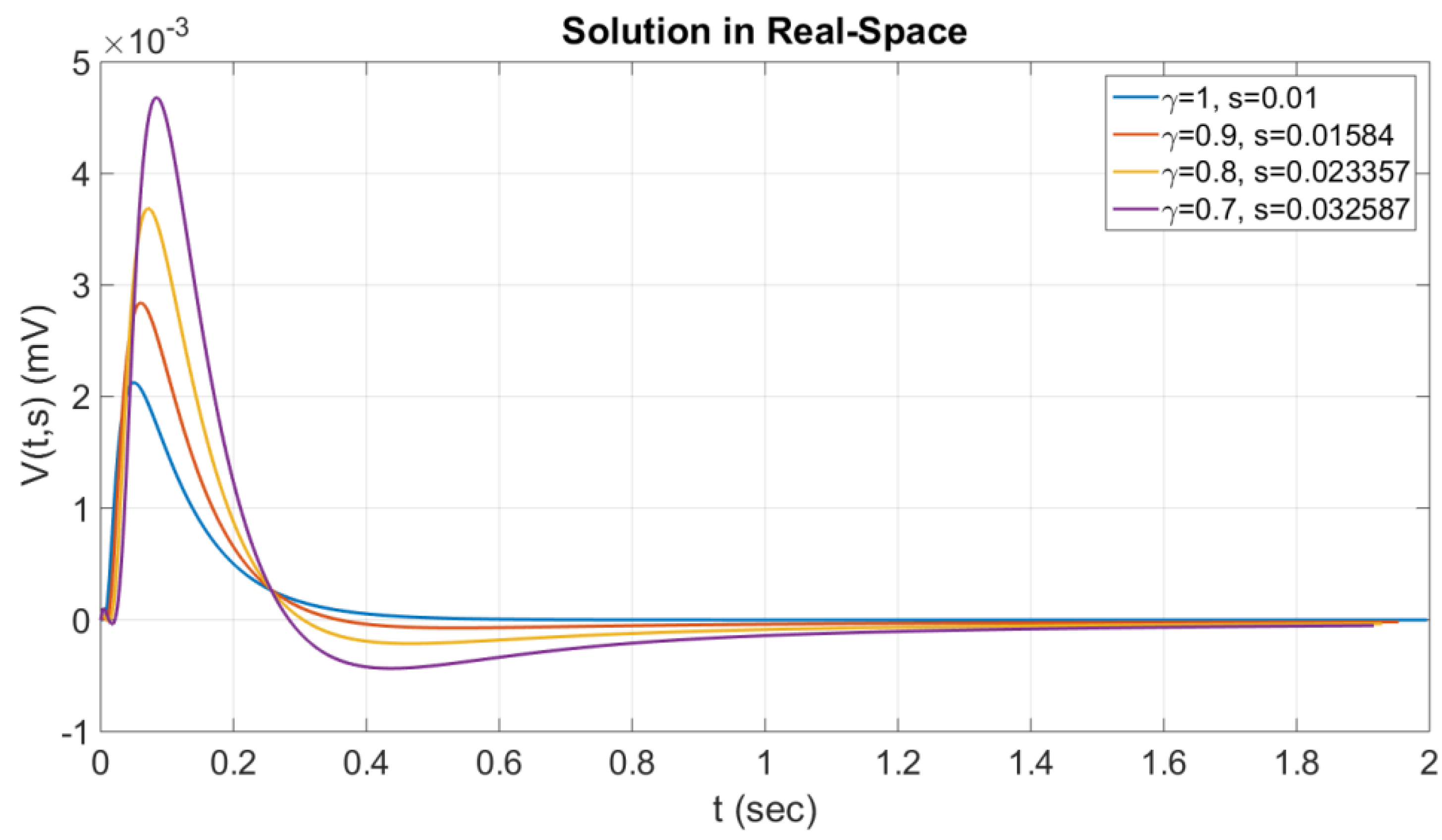
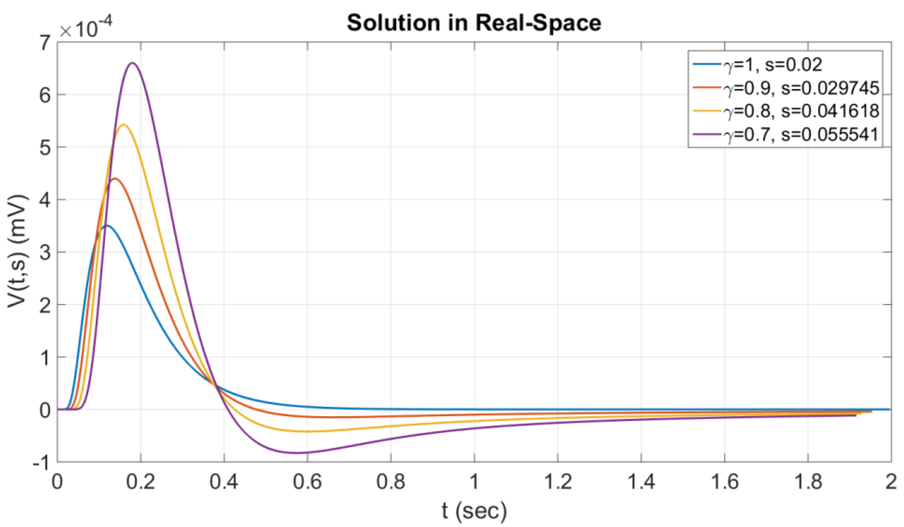
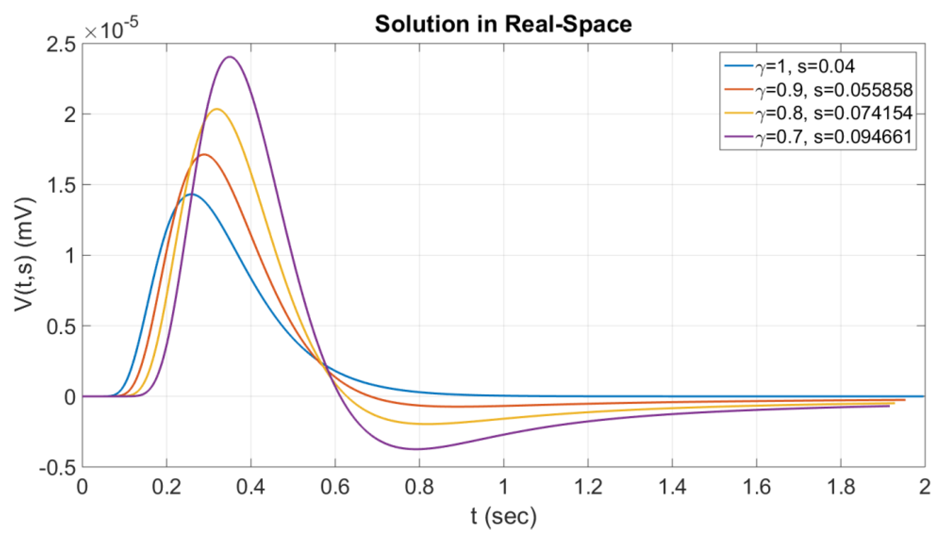
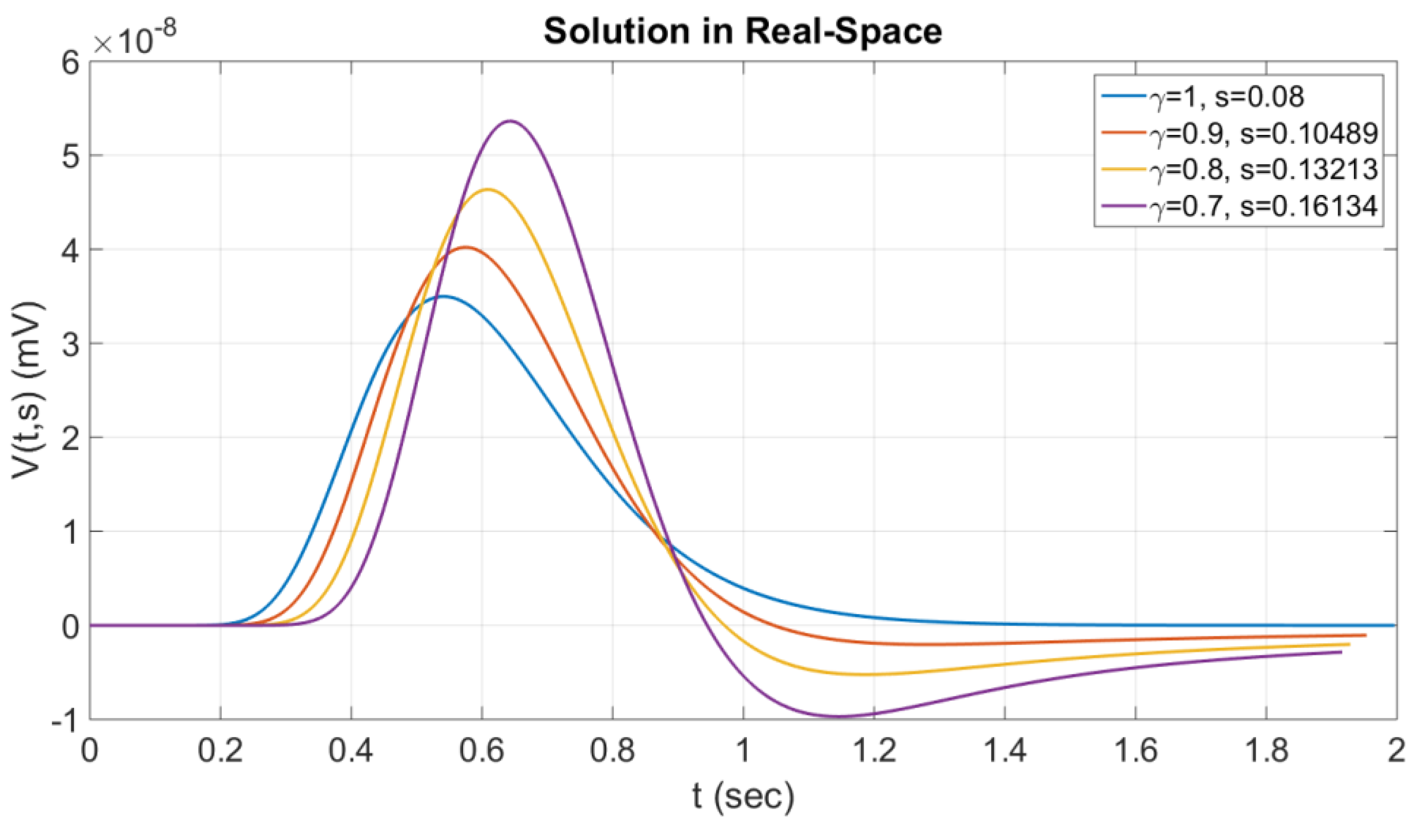
The results for voltage V(t, s) for various values of s and fractional order γ in real space are shown in Figure 1, Figure 2, Figure 3 and Figure 4. In these figures, we can see that as the value of arc length s increases, we shift the voltage’s maximum to higher time values. We believe this delay in maximum response is expected due to increased cable length. Also, for the same reason, we have a decrease in the maximum value of voltage and broadness of the voltage curve as the arc length s increases, denoting an inertial behavior across the cable.

Finally, we must mention that in all cases of arc length values, the decrease of fractional order γ gives greater maximum values in voltage and reverses the polarity of the resulting voltage (from positive values to negative ones) as time passes.

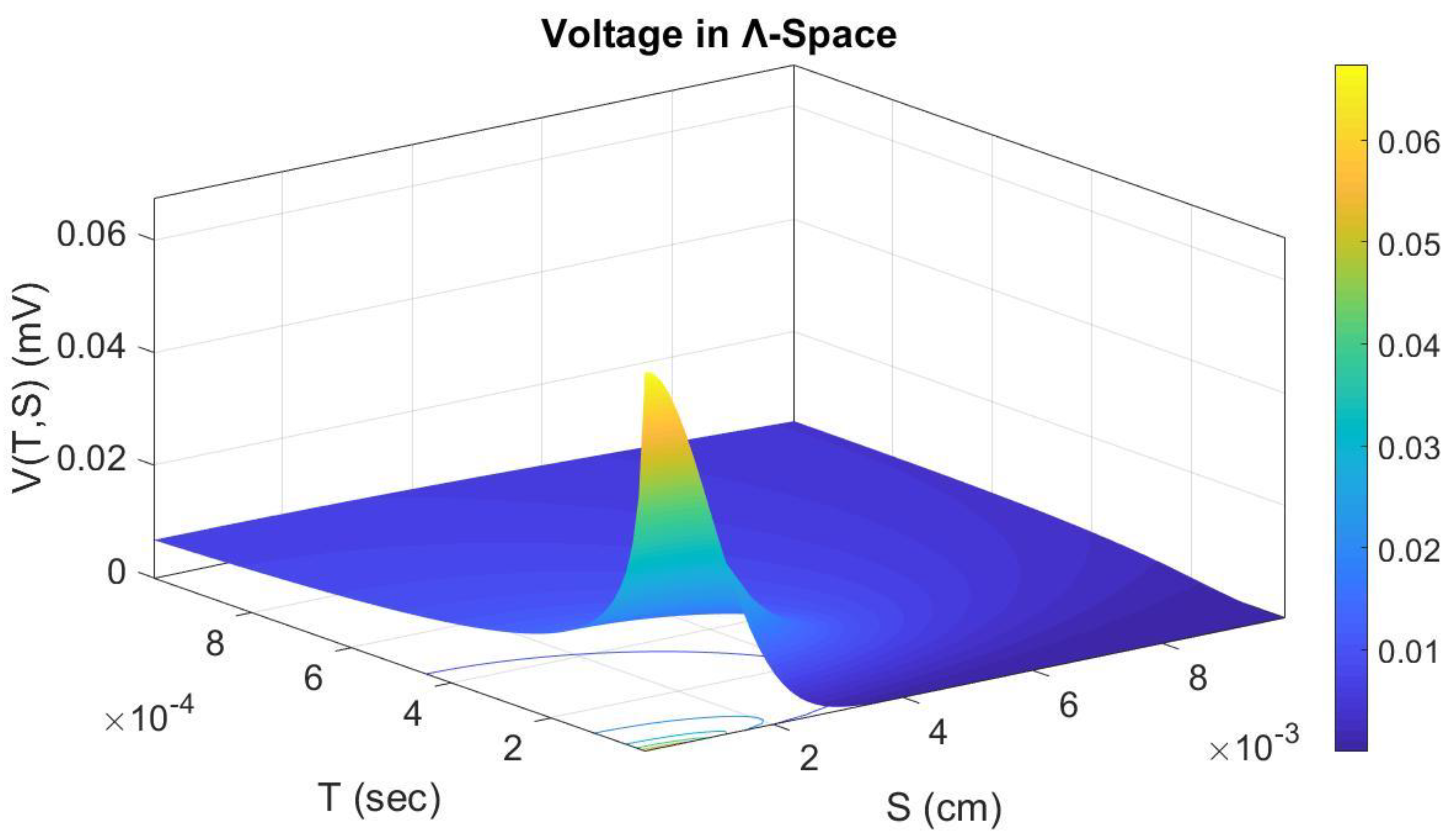
Now, we will examine the voltage V^Λ(T,S) (Equation (12)) as a two-variable function in Λ-space. In order to transform it to the initial space, we will use the following formula of inverse transformation for both t and s, according to K. Lazopoulos’ [11] fractional approach:

$$V(t,s)={}_0{}^{RL}D{}_t^{1-{\gamma }_2}({}_0{}^{RL}D{}_s^{1-{\gamma }_1}(V^{\Lambda }(\tau ,q)))=\frac{1}{\Gamma ({\gamma }_2)\cdot \Gamma ({\gamma }_1)}\cdot \frac{d}{dt}{\displaystyle {\int }_0^t\frac{1}{{(t-\tau )}^{1-{\gamma }_2}}}(\frac{d}{ds}{\displaystyle {\int }_0^s\frac{V^{\Lambda }(\tau ,q)}{{(s-q)}^{1-{\gamma }_1}}}dq)d\tau$$

(15)

where the relation gives V^Λ (τ,q):

$$V^{\Lambda }\left(\tau ,q\right)=V_0{l}_0\sqrt{\frac{r_L\cdot c_M\cdot \Gamma \left(3-{\gamma }_2\right)}{2\cdot \pi \cdot R_0\cdot {\tau }^{2-{\gamma }_2}}}\cdot e^{-\frac{r_L\cdot c_M\cdot \Gamma \left(3-{\gamma }_2\right)\cdot q^{4-2{\gamma }_1}}{2R_0\cdot {(\Gamma \left(3-{\gamma }_1\right))}^2\cdot {\tau }^{2-{\gamma }_2}}}\cdot e^{-\frac{{\tau }^{2-{\gamma }_2}}{r_L\cdot c_M\cdot \Gamma \left(3-{\gamma }_2\right)}}$$

(16)

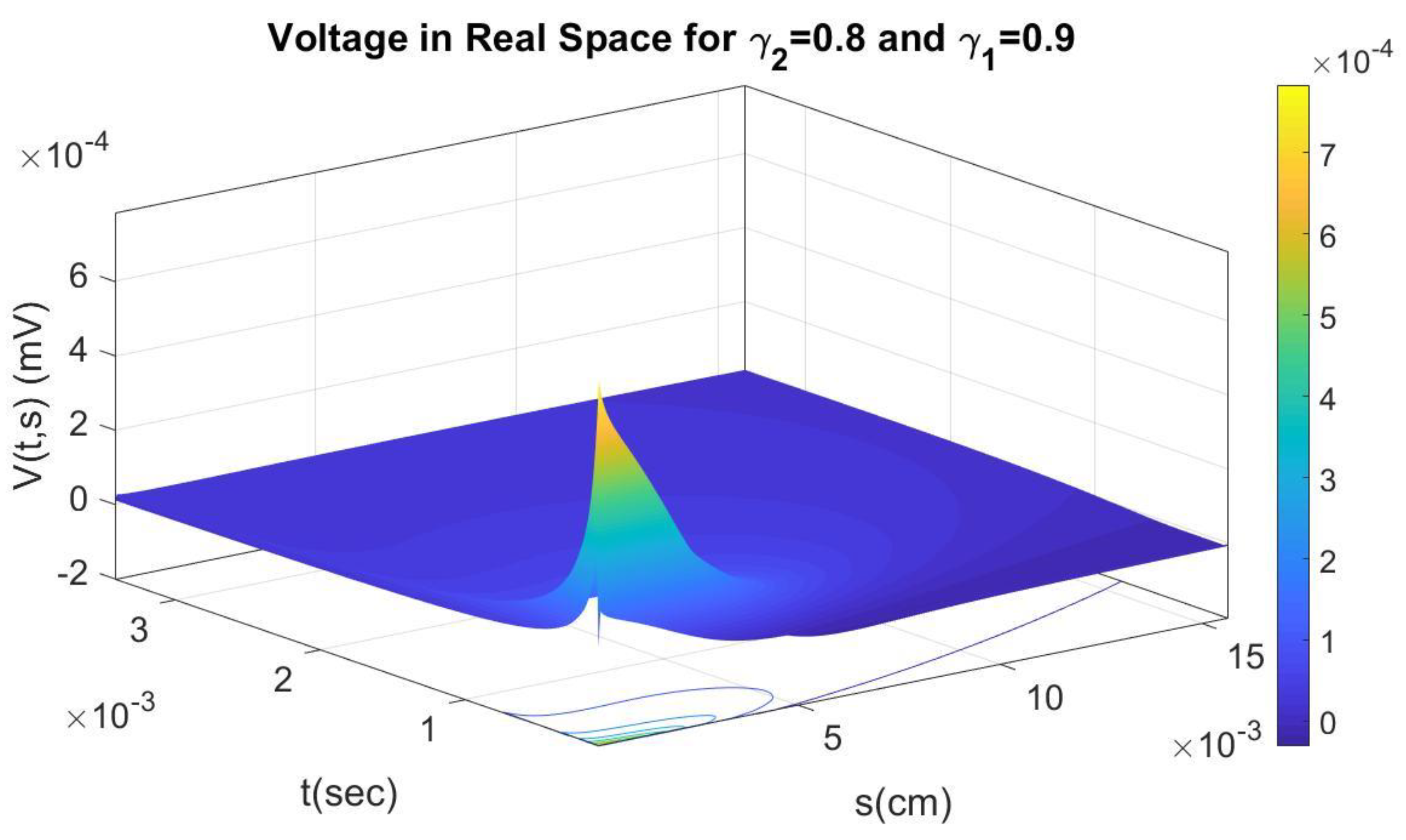
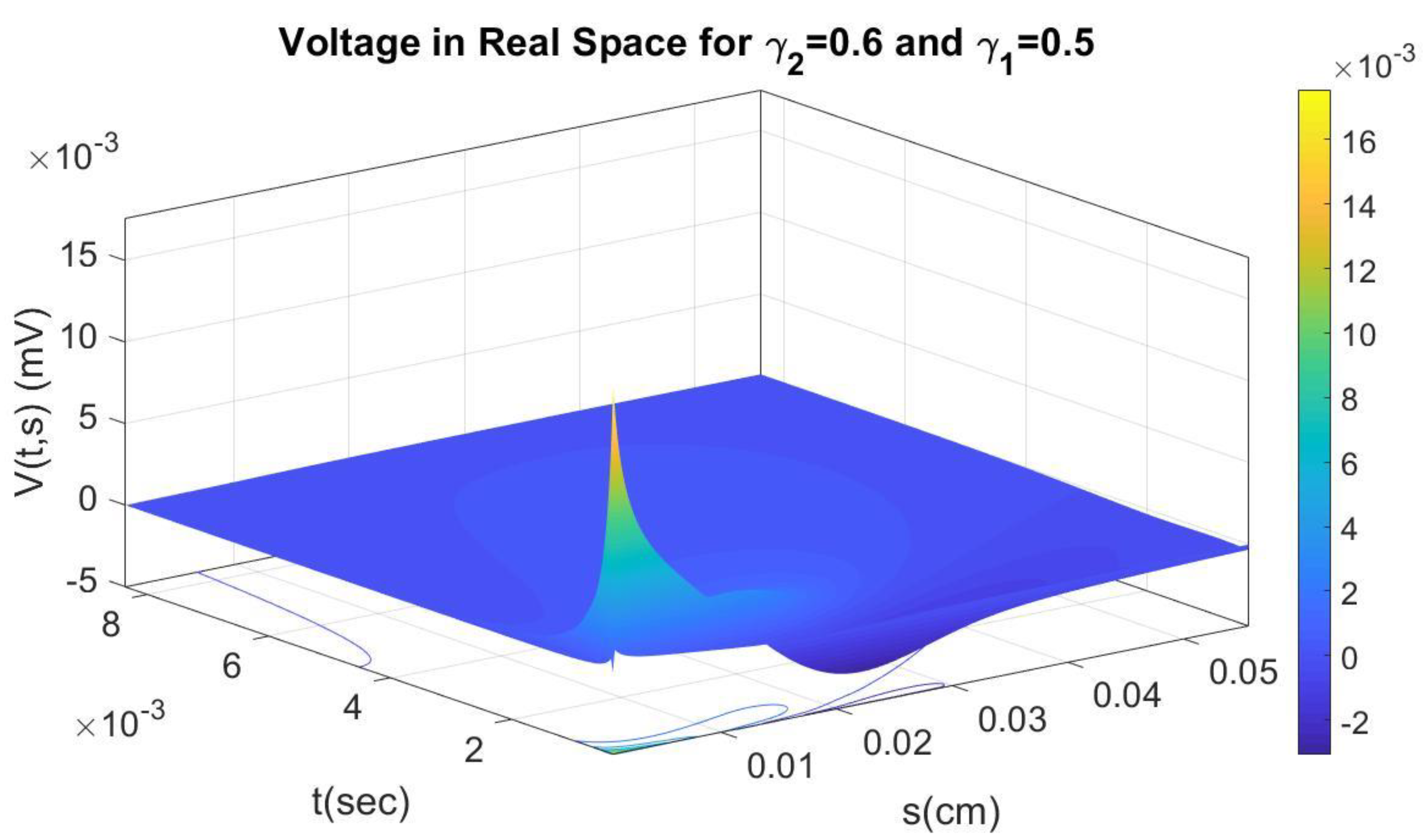
Here, the fractional orders (γ₂,γ₁) for the inverse transformation are different for time t and arc length s. Figure 5, Figure 6, Figure 7, Figure 8, Figure 9, Figure 10 and Figure 11 present the voltage V(t,s) in real space for various values of fractional orders. The constants in Equation (16) take the same values as in Equation (12).

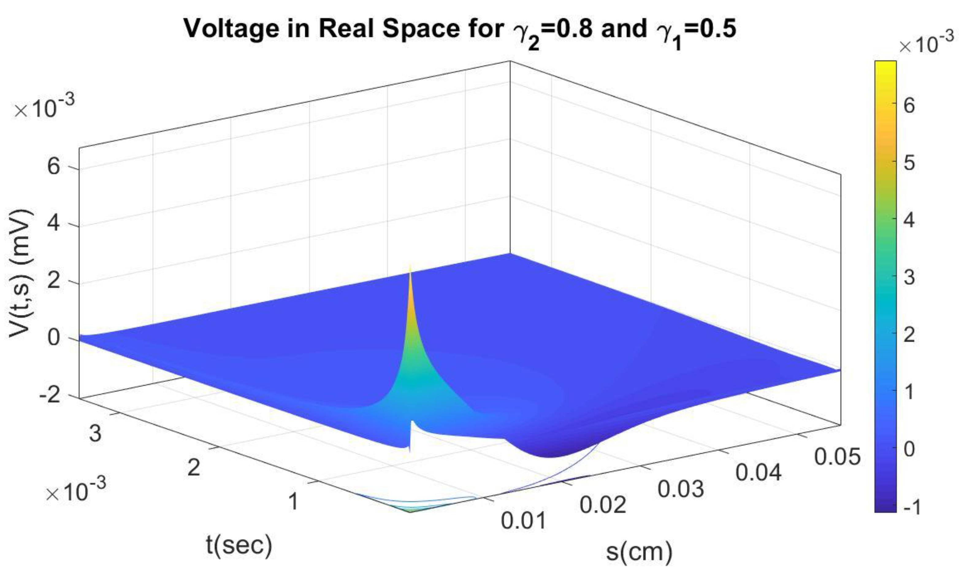
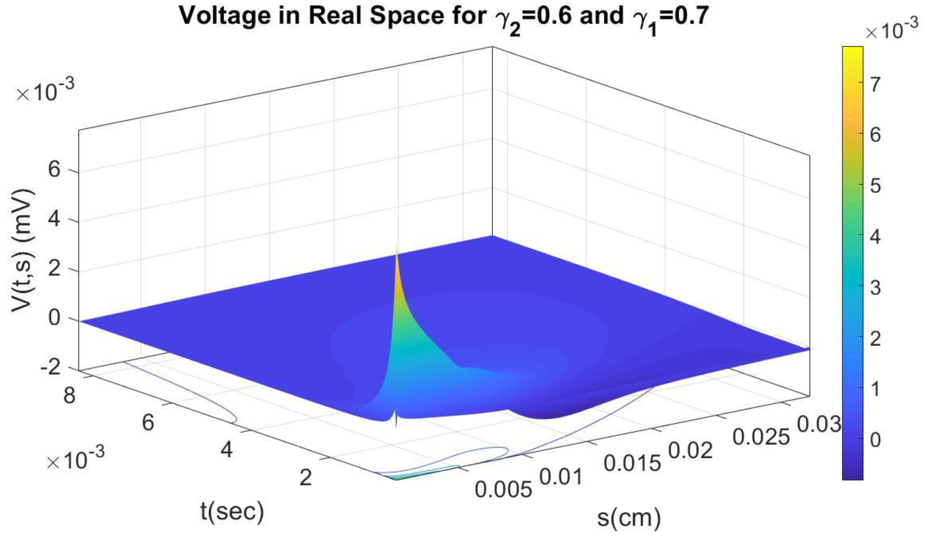
Based on Figure 5, Figure 6, Figure 7, Figure 8, Figure 9, Figure 10 and Figure 11, we can indeed conclude that as the fractional order for time t (γ₂) or arc length s (γ₁) decreases, the maximum value reached by the voltage V(t,s) increases. Also, in all cases, we have a change in the polarity of the voltage (positive to negative) along the cable. Finally, we can observe that as fractional order for time t (γ₂) or arc length s (γ₁) decreases, we have non-zero voltage values for higher values of arc length s (longer cable).

4. Conclusions

Dendrites and axons are modeled as cables using fractional calculus. The voltage potential is transferred from Λ-space to the initial space. During this procedure, many interesting conclusions can be addressed, such as the high influence of the length of the cable s and the critical impact of the fractional order. More precisely, an increasing s results in the increase of voltage, while the decrease in fractional order also increases the voltage. The present work is addressed to medical and bioengineering researchers for controlling the evolution of various brain diseases, refs. [16,17,18,19].

References

- Drapaca, C.S.; Sivaloganathan, S.A. Fractional model of continuum mechanics. J. Elast. 2012, 107, 107–123. [Google Scholar] [CrossRef]
- Di Paola, M.; Failla, G.; Zingales, M. Physically-based approach to the mechanics of strong non-local linear elasticity theory. J. Elast. 2009, 97, 103–130. [Google Scholar] [CrossRef]
- Carpinteri, A.; Cornetti, P.; Sapora, A. A Fractional calculus approach to non-local elasticity. Eur. Phys. J. Spec. Top. 2011, 193, 193–204. [Google Scholar] [CrossRef]
- Magin, R.L. Fractional calculus in bioengineering, Parts 1–3. Crit. Rev. Biomed. Eng. 2004, 32, 1–377. [Google Scholar] [CrossRef] [PubMed] [Green Version]
- Hilfer, R. Applications of Fractional Calculus in Physics; World Scientific: River Edge, NJ, USA, 2000. [Google Scholar]
- West, B.J.; Bologna, M.; Grigolini, P. Physics of Fractal Operators; Springer: New York, NY, USA, 2003. [Google Scholar]
- Eringen, A.C. Nonlocal Continuum Field Theories; Springer: New York, NY, USA, 2002. [Google Scholar]
- Kilbas, A.A.; Srivastava, H.M.; Trujillo, J.J. Theory and Applications of Fractional Differential Equations; Elsevier: Amsterdam, The Netherlands, 2006. [Google Scholar]
- Podlubny, I. Fractional Differential Equations (An Introduction to Fractional Derivatives, Fractional Differential Equations, Some Methods of Their Solution and Some of Their Applications); Academic Press: San Diego, CA, USA; Boston, MA, USA; New York, NY, USA; London, UK; Tokyo, Japan; Toronto, ON, Canada, 1999. [Google Scholar]
- Chillingworth, D. Differential Topology with a View to Applications; Pitman: London, UK; San Francisco, CA, USA, 1976. [Google Scholar]
- Lazopoulos, K.A.; Lazopoulos, A.K. On the Mathematical Formulation of Fractional Derivatives. Prog. Fract. Differ. Appl. 2019, 5, 261–267. [Google Scholar]
- Samko, S.G.; Kilbas, A.A.; Marichev, O.I. Fractional Integrals and Derivatives: Theory and Applications; Gordon and Breach: Amsterdam, The Netherlands, 1993. [Google Scholar]
- Oldham, K.B.; Spanier, J. The Fractional Calculus; Academic Press: New York, NY, USA; London, UK, 1974. [Google Scholar]
- Mainardi, F. Fractional Calculus and Waves in Linear Viscoelasticity; Imperial College Press: London, UK, 2010. [Google Scholar]
- Lopez-Sanchez, E.J.; Romero, J.M. Cable equation for general geometry. Phys. Rev. E 2017, 95, 022403. [Google Scholar] [CrossRef] [PubMed] [Green Version]
- Haugh, J.M. Analysis of reaction-diffusion systems with anomalous subdiffusion. Biophys. J. 2009, 97, 435–442. [Google Scholar] [CrossRef] [PubMed] [Green Version]
- Saxon, M.J. A biological interpretation of transient anomalous subdiffusion. I, Qualitative model. Biophys. J. 2007, 92, 1178–1191. [Google Scholar] [CrossRef] [PubMed] [Green Version]
- Weiss, M.; Elsner, M.; Kartberg, F.; Nilsson, T. Anomalous subdiffusion is a measure for cytoplasmic crowding in living cells. Biophys. J. 2004, 87, 3518–3524. [Google Scholar] [CrossRef] [PubMed] [Green Version]
- Saxon, M.J. Anomalous subdiffusion in fluorescence photobleaching recovery: A Monte Carlo study. Biophys. J. 2001, 81, 2226–2240. [Google Scholar] [CrossRef] [PubMed]
Figure 1.
The voltage V(t,s) for various values of fractional order γ and corresponding values of s in real space (S = 0.01).
Figure 2.
The voltage V(t,s) for various values of fractional order γ and corresponding values of s in real space (S = 0.02).
Figure 3.
The voltage V(t,s) for various values of fractional order γ and corresponding values of s in real space (S = 0.04).
Figure 4.
The voltage V(t,s) for various values of fractional order γ and corresponding values of s in real space (S = 0.08).
Figure 5.
The voltage VΛ(T,S) in Λ-space as a function of time T and arc length S.
Figure 6.
The voltage V(t,s) in real space as a function of time and arc length s, for fractional orders γ2 = 0.8 and γ1 = 0.9.
Figure 7.
The voltage V(t,s) in real space as a function of time and arc length s, for fractional orders γ2 = 0.8 and γ1 = 0.7.
Figure 8.
The voltage V(t,s) in real space as a function of time and arc length s, for fractional orders γ2 = 0.8 and γ1 = 0.5.
Figure 9.
The voltage V(t,s) in real space as a function of time and arc length s, for fractional orders γ2 = 0.6 and γ1 = 0.9.
Figure 10.
The voltage V(t,s) in real space as a function of time and arc length s, for fractional orders γ2 = 0.6 and γ1 = 0.7.
Figure 11.
The voltage V(t,s) in real space as a function of time and arc length s, for fractional orders γ2 = 0.6 and γ1 = 0.5.
Disclaimer/Publisher’s Note: The statements, opinions and data contained in all publications are solely those of the individual author(s) and contributor(s) and not of MDPI and/or the editor(s). MDPI and/or the editor(s) disclaim responsibility for any injury to people or property resulting from any ideas, methods, instructions or products referred to in the content. |
© 2023 by the authors. Licensee MDPI, Basel, Switzerland. This article is an open access article distributed under the terms and conditions of the Creative Commons Attribution (CC BY) license (https://creativecommons.org/licenses/by/4.0/).
Share and Cite
MDPI and ACS Style
Karaoulanis, D.; Lazopoulos, A.K.; Lazopoulou, N.; Lazopoulos, K. On Λ-Fractional Derivative and Human Neural Network. Axioms 2023, 12, 136. https://doi.org/10.3390/axioms12020136
AMA Style
Karaoulanis D, Lazopoulos AK, Lazopoulou N, Lazopoulos K. On Λ-Fractional Derivative and Human Neural Network. Axioms. 2023; 12(2):136. https://doi.org/10.3390/axioms12020136
Chicago/Turabian StyleKaraoulanis, D., A. K. Lazopoulos, N. Lazopoulou, and K. Lazopoulos. 2023. "On Λ-Fractional Derivative and Human Neural Network" Axioms 12, no. 2: 136. https://doi.org/10.3390/axioms12020136
Note that from the first issue of 2016, this journal uses article numbers instead of page numbers. See further details here.