On the Convergence Properties of a Stochastic Trust-Region Method with Inexact Restoration

Abstract

We study the convergence properties of SIRTR, a stochastic inexact restoration trust-region method suited for the minimization of a finite sum of continuously differentiable functions. This method combines the trust-region methodology with random function and gradient estimates formed by subsampling. Unlike other existing schemes, it forces the decrease of a merit function by combining the function approximation with an infeasibility term, the latter of which measures the distance of the current sample size from its maximum value. In a previous work, the expected iteration complexity to satisfy an approximate first-order optimality condition was given. Here, we elaborate on the convergence analysis of SIRTR and prove its convergence in probability under suitable accuracy requirements on random function and gradient estimates. Furthermore, we report the numerical results obtained on some nonconvex classification test problems, discussing the impact of the probabilistic requirements on the selection of the sample sizes.

1. Introduction

The solutions of large-scale finite-sum optimization problems have become essential in several machine learning tasks including binary or multinomial classification, regression, clustering, and anomaly detection [1,2]. Indeed, the training of models employed in such tasks is often performed by solving the optimization

$$\underset{x\in {\mathbb{R}}^n}{min}{f}_N\left(x\right)=\frac{1}{N}\sum _{i=1}^N{\varphi }_i\left(x\right),$$

(1)

where N is the size of the available data set and the functions ${\varphi }_i:{\mathbb{R}}^n\to \mathbb{R}$ are continuously differentiable for all $i=1,\dots ,N$. As a result, the efficient solution of a machine learning problem calls for efficient numerical algorithms for (1).

When the data set is extremely large, the evaluation of the objective function $f_N$ and its derivatives may be computationally demanding, making deterministic optimization methods inadequate for solving (1). A common strategy consists of approximating both the function and derivatives by employing a small number of loss functions ${\varphi }_i$ sampled randomly, making stochastic optimization methods the preferred choice [3,4,5]. A major issue is the sensitivity of most stochastic algorithms to their parameters, such as the learning rate or sample sizes used for building the function and gradient approximations, which usually need to be tuned through multiple trials and errors before the algorithm exhibits acceptable performance. A possible remedy to burdensome tuning is to employ adaptive optimization methods, which compute the parameters according to appropriate globalization strategies [6,7,8,9,10,11,12,13,14,15,16,17,18,19,20]. Most of these methods have probabilistic accuracy requirements for the function and gradient estimates in order to ensure either the iteration complexity of the expectation [7,8,9,10,11,13,15,19,21,22] or the convergence in probability of the iterates [6,12,16,17,18,20]. In turn, these requirements are reflected in the choice of sample size, which needs to progressively grow as the iterations proceed, resulting in an increasing computational cost per iteration.

In [11], the authors proposed the so-called stochastic inexact restoration trust-region (SIRTR) method for solving (1). SIRTR employs subsampled function and gradient estimates and combines the classical trust-region scheme with the inexact restoration method for constrained optimization problems [23,24,25]. This combined strategy involves the reformulation of (1) as an optimization problem with two unknown variables $x,M$, where x is the object to be recovered and M is the sample size of the function estimate, upon which the constraint $M=N$ is imposed. Based on this reformulation of (1), the method acts on the two variables in a modular way: first, it selects the sample size with a deterministic rule aimed at improving feasibility with respect to the constraint $M=N$; then, it accepts or rejects the inexact trust-region step by improving optimality with respect to a suitable merit function. SIRTR has shown good numerical performance on a series of classification and regression test problems, as its inexact restoration strategy drastically reduces the computational burden due to the selection of the algorithmic parameters. From a theoretical viewpoint, the authors in [11] provided an upper bound on the expected number of iterations to reach a near-stationary point under some appropriate probability accuracy requirements on the random estimators; remarkably, such requirements are less stringent than others employed in the literature. However, the convergence in probability of SIRTR remains unproved, thus leaving open the question of whether the gradient of the objective function in (1) converges to zero with a probability of one. A positive answer to this question would be an important theoretical confirmation of the numerical stability of the method.

In this paper, we improve on the existing theoretical analysis of SIRTR, showing that its iterates drive the gradient to zero with a probability of one. The results will be obtained by combining the theoretical properties of SIRTR with some tools from martingale theory, as typically done for the convergence analysis of adaptive stochastic methods [6,16,18]. Furthermore, we show the numerical results obtained by applying SIRTR on nonconvex binary classification, discussing the impact of the probabilistic accuracy requirements on the performance of the method.

The paper is structured as follows. In Section 2, we briefly outline the method and its main steps. In Section 3, we perform the convergence analysis of the method, showing that its iterates converge with a probability of one. In Section 4, we provide a numerical illustration of a binary classification test problem. Finally, we report the conclusions and future work in Section 5.

Notations: Throughout the paper, $\mathbb{R}$ is the set of real numbers, whereas the symbol $\parallel ·\parallel$ denotes the standard Euclidean norm on ${\mathbb{R}}^n$. We denote with $(\mathrm{\Omega },\mathcal{A},\mathbb{P})$ a probability space, where $\mathrm{\Omega }$ is the sample space, $\mathcal{A}\subseteq \mathcal{P}\left(\mathrm{\Omega }\right)$ is the $\sigma -$ algebra of events, and $\mathbb{P}:\mathcal{A}\to [0,1]$ is the probability function. Given an event $A\in \mathcal{A}$, the symbol $\mathbb{P}\left(A\right)$ stands for the probability of the event A, and ${𝟙}_A:\mathrm{\Omega }\to \{0,1\}$ denotes the indicator function of an event A, i.e., the function such that ${𝟙}_A\left(\omega \right)=1$ if $\omega \in A$, or ${𝟙}_A\left(\omega \right)=0$ otherwise. Given a random variable $X:\mathrm{\Omega }\to \mathbb{R}$, we denote with $\mathbb{E}\left(X\right)$ the expected value of X. Let $X_1,\dots ,X_n$ be n random variables, and the notation $\sigma (X_1,\dots ,X_n)$ stands for the $\sigma -$ algebra generated by $X_1,\dots ,X_n$.

2. The SIRTR Method

Here, we present the stochastic inexact restoration trust-region (SIRTR) method, which was formerly proposed in [11]. SIRTR is a trust-region method with subsampled function and gradient estimates, which combines first-order trust-region methodology with the inexact restoration method for constrained optimization [25]. In order to provide a detailed description of SIRTR, we reformulate (1) as the constrained problem

$$\begin{array}{cc}\hfill & \underset{x\in {\mathbb{R}}^n}{min}{f}_M\left(x\right)=\frac{1}{M}\sum _{i\in I_M}{\varphi }_i\left(x\right),\hfill \\ \hfill & \mathrm{s}.\mathrm{t}.M=N\hfill \end{array}$$

(2)

where $I_M\subseteq \{1,\dots ,N\}$ is a sample set of the size of the cardinality $|I_M|$ such that $|I_M|=M$. To measure the infeasibility distance of M from the constraint $M=N$, we introduce a function h that measures the distance of $M\in \{1,\dots ,N\}$ from N. Function h is supposed to satisfy the following properties.

Assumption 1.

The function $h:\{1,2,\dots ,N\}\to \mathbb{R}$ is monotonically decreasing and satisfies $h\left(1\right)>0$, $h\left(N\right)=0$.

From Assumption 1, the existence of some positive constants $\underline{h}$ and $\overline{h}$ follows such that

$$\underline{h}\le h\left(M\right)\le \overline{h},\mathrm{for}1\le M\le N.$$

(3)

An example of a function $h:\{1,\dots ,N\}\to \mathbb{R}$ satisfying Assumption 1 is $h\left(M\right)=\frac{N-M}{N}$.

SIRTR is a stochastic variant of the classical first-order trust-region method, which accepts the trial point according to the decrease of a convex combination of the function estimate $f_M$ with function h. We report SIRTR in Algorithm 1.

At the beginning of each iteration $k\ge 0$, we have at our disposal the iterate $x_k$, the trust-region radius ${\delta }_k$, the sample size $N_k\in \{1,\dots ,N\}$, the penalty parameter ${\theta }_k$, and the flag iflag, where iflag = succ if the previous iteration was successful, in the sense that is specified below, and iflag = unsucc otherwise. Then, in Steps 1–5, perform the following tasks.

• In Step 1, if iflag = succ, we reduce the current value $h\left(N_k\right)$ of the infeasibility measure and find some ${\tilde{N}}_{k+1}\in \{1,\dots ,N\}$ satisfying $h({\tilde{N}}_{k+1})\le rh(N_k)$ with $r\in (0,1)$. On the other hand, if iflag=unsucc, ${\tilde{N}}_{k+1}$ remains the same from one iteration to the other, i.e., we set ${\tilde{N}}_{k+1}={\tilde{N}}_k$. Note that ${\tilde{N}}_{k+1}=N$ if $N_k=N$.
• Step 2 determines a trial sample size $N_{k+1}^t$ that satisfies $h(N_{k+1}^t)-h({\tilde{N}}_{k+1})\le \mu {\delta }_k^2$ with $\mu >0$ and is used to form the random model. In principle, we could fix $N_{k+1}^t={\tilde{N}}_{k+1}$, but selecting a smaller sample size, if possible, yields a computational saving in the successive step. The relation between $N_{k+1}^t$ and ${\tilde{N}}_{k+1}$ depends on ${\delta }_k$; small values of ${\delta }_k$ give $N_{k+1}^t={\tilde{N}}_{k+1}$; otherwise, $N_{k+1}^t$ is allowed to be smaller than ${\tilde{N}}_{k+1}$.
• Step 3 forms the random model $m_k(p)$ and the trial step $p_k$. The linear model is given by $m_k(p)=f_{N_{k+1}^t}(x_k)+g_k^{T}p$, where

  $$f_{N_{k+1}^t}(x_k)=\frac{1}{N_{k+1}^t}\sum _{i\in I_{N_{k+1}^t}}{\varphi }_i(x_k),$$

  (4)

  and

  $$g_k=\frac{1}{N_{k+1,g}}\sum _{i\in I_{N_{k+1,g}}}\nabla {\varphi }_i(x_k),$$

  (5)

  with $I_{N_{k+1,g}}\subset \{1,\dots ,N\}$ with cardinality $|I_{N_{k+1,g}}|=N_{k+1,g}$.

Minimizing $m_k$ over the ball of center 0 and radius ${\delta }_k$ gives the trial step

$$p_k=\underset{\parallel p\parallel \le {\delta }_k}{argmin}{m}_k(p)=-{\delta }_k\frac{g_k}{\parallel g_k\parallel }.$$

Algorithm 1 Stochastic Inexact Restoration Trust-Region (SIRTR)

Given $x_0\in {\mathbb{R}}^n$, $N_0\in \{1,\dots ,N\}$, ${\eta }_1\in (0,1)$, ${\theta }_0\in (0,1)$, $r\in (0,1)$, $\gamma >1$, $\mu >0$, ${\eta }_2>0$, $0<{\delta }_0<{\delta }_{max}$.

0. Set $k=0$, iflag=succ. 1. Reference sample size If iflag=succ       find ${\tilde{N}}_{k+1}$ such that $N_k\le {\tilde{N}}_{k+1}\le N$ and $$h({\tilde{N}}_{k+1})\le rh(N_k),$$ (6) Else       set ${\tilde{N}}_{k+1}={\tilde{N}}_k$. 2. Trial sample size If $N_k=N$       set $N_{k+1}^t=N$ Else       find $N_{k+1}^t$ such that $$\begin{array}{ccc}\hfill h(N_{k+1}^t)-h({\tilde{N}}_{k+1})& \le & \mu {\delta }_k^2.\hfill \end{array}$$ (7) 3. Trust-region model Choose $I_{N_{k+1}^t}\subseteq \{1,\dots ,N\}$ such that $\left|I_{N_{k+1}^t}\right|=N_{k+1}^t$. Choose $N_{k+1,g}$ and $I_{N_{k+1,g}}\subseteq \{1,\dots ,N\}$ such that $\left|I_{N_{k+1,g}}\right|=N_{k+1,g}$. Compute $g_k$ as in (5), and set $p_k=-{\delta }_k\frac{g_k}{\parallel g_k\parallel }$. Compute $f_{N_{k+1}^t}(x_k)$ as in (4), and set $m_k(p_k)=f_{N_{k+1}^t}(x_k)+g_k^T{p}_k$. 4. Penalty parameter If ${\mathrm{Pred}}_k({\theta }_k)\ge {\eta }_1(h(N_k)-h({\tilde{N}}_{k+1}))$       set $${\theta }_{k+1}={\theta }_k$$ Else       set $${\displaystyle {\theta }_{k+1}=\frac{(1-{\eta }_1)(h(N_k)-h({\tilde{N}}_{k+1}))}{m_k(p_k)-f_{N_k}(x_k)+h(N_k)-h({\tilde{N}}_{k+1})}.}$$ (8) 5. Acceptance test If ${Ared}_k(x_k+p_k,{\theta }_{k+1})\ge {\eta }_1{Pred}_k({\theta }_{k+1})$ and $\parallel g_k\parallel \ge {\eta }_2{\delta }_k$ (success)      define $$\begin{array}{cc}\hfill x_{k+1}& =x_k+p_k\hfill \\ \hfill {\delta }_{k+1}& =min\left\{\gamma {\delta }_k,{\delta }_{max}\right\}\hfill \end{array}$$ (9)       set $N_{k+1}=N_{k+1}^t$, $k=k+1$, iflag=succ and go to Step 1. Else (unsuccess)      define $$\begin{array}{cc}\hfill x_{k+1}& =x_k\hfill \\ \hfill {\delta }_{k+1}& =\frac{{\delta }_k}{\gamma },\hfill \end{array}$$ (10)       set $N_{k+1}=N_k$, $k=k+1$, iflag=unsucc and go to Step 1.

• In Step 4, we compute the penalty parameter ${\theta }_{k+1}\in (0,1)$ that governs the predicted reduction ${Pred}_k$ in the function and infeasibility measure, which we define as

  $${Pred}_k(\theta )=\theta (f_{N_k}(x_k)-m_k(p_k))+(1-\theta )(h(N_k)-h({\tilde{N}}_{k+1})).$$

  (11)

If $\theta ={\theta }_k$ satisfies

$${Pred}_k(\theta )\ge {\eta }_1(h(N_k)-h({\tilde{N}}_{k+1})),$$

(12)

then, we set ${\theta }_{k+1}={\theta }_k$; otherwise, we compute ${\theta }_{k+1}$ as the biggest value for which Inequality (12) is satisfied and takes the explicit form given in (8).

• In Step 5, we establish if we accept (success) or reject (unsuccess) the trial point $x_k+p_k$. The actual reduction ${Ared}_k$ at point $\widehat{x}$ is defined as

  $${Ared}_k(\widehat{x},\theta )=\theta (f_{N_k}(x_k)-f_{N_{k+1}^t}(\widehat{x}))+(1-\theta )(h(N_k)-h(N_{k+1}^t)),$$

  (13)

  and we declare a successful iteration whenever the following conditions are both met:

  $$\begin{array}{cc}\hfill {Ared}_k(x_k+p_k,{\theta }_{k+1})& \ge {\eta }_1{Pred}_k({\theta }_{k+1})\hfill \end{array}$$

  (14)

  $$\begin{array}{cc}\hfill \parallel g_k\parallel & \ge {\eta }_2{\delta }_k.\hfill \end{array}$$

  (15)

  Condition (14) reduces to the standard acceptance criterion of deterministic trust-region methods when $N_k={\tilde{N}}_{k+1}=N_{k+1}^t=N$. If both conditions are satisfied, we accept the step $p_k$ and set $x_{k+1}=x_k+p_k$, increase the trust-region radius based on the update rule (9), and set $N_{k+1}=N_{k+1}^t$, iflag=succ; otherwise, we retain the previous iterate, i.e., $x_{k+1}=x_k$, reduce the trust-region radius according to (10), and set $N_{k+1}=N_k$, iflag = unsucc.

3. Convergence Analysis

In this section, we are interested in the convergence properties of Algorithm 1. To this aim, we note that the function estimates $f_{N_{k+1}^t}(x_k)$ in (4) and gradient estimates $g_k$ in (5) are all random quantities. Consequently, Algorithm 1 generates a random process, that is, the iterates $X_k$, the trust region radii ${\Delta }_k$, the gradient estimates $G_k,\nabla f_{N_{k+1}^t}(X_k)$, and the values ${\mathrm{\Psi }}_k$ of the Lyapunov function $\mathrm{\Psi }$ in (21) at iteration k are to be considered as random variables, with their realizations denoted as $x_k$, ${\delta }_k$, $g_k$, and ${\psi }_k$.

Our aim is to show the convergence in probability of the iterates generated by Algorithm 1, in the sense that

$$\mathbb{P}\left(\underset{k\to \infty }{lim}\parallel \nabla f(X_k)\parallel =0\right)=1,$$

(16)

i.e., the event ${lim}_{k\to \infty }\parallel \nabla f(X_k)\parallel =0$ holds almost surely. We note that the authors in [11] derived a bound on the expected number of iterations in Algorithm 1 required to reach the desired accuracy in the gradient norm, but did not show the convergence results of Type (16).

3.1. Preliminary Results

We recall some technical preliminary results that were obtained for Algorithm 1 in [11]. First, we impose some basic assumptions on the functions in Problem (1).

Assumption 2.

(i) 

Each function ${\varphi }_i:{\mathbb{R}}^n\to \mathbb{R}$ is continuously differentiable for $i=1,\dots ,N$.

(ii) 

The functions $f_M:{\mathbb{R}}^n\to \mathbb{R}$, $M=1,\dots ,N$, are bounded from below on ${\mathbb{R}}^n$, i.e., there exists $f_{low}\in \mathbb{R}$ such that

$$f_M(x)\ge f_{low},1\le M\le N,x\in {\mathbb{R}}^n.$$

(iii) 

The functions $f_M:{\mathbb{R}}^n\to \mathbb{R}$, $M=1,\dots ,N$, are bounded from above on a subset $\mathrm{\Omega }\subseteq {\mathbb{R}}^n$, i.e., there exists $f_{up}\in \mathbb{R}$ such that

$$f_M(x)\le f_{up},1\le M\le N,x\in \mathrm{\Omega }.$$

Furthermore, the iterates ${\left\{x_k\right\}}_{k\in \mathbb{N}}$ defined by Algorithm 1 are contained in Ω.

Combining Step 4 of Algorithm 1 with Bound (3) and Assumption 2(iii), it is possible to prove that for any realizations of the algorithm, the sequence ${\left\{{\theta }_k\right\}}_{k\in \mathbb{N}}$ is bounded away from zero.

Lemma 1 

([11], Lemma 2). Let Assumptions 1 and 2 hold and consider a particular realization of Algorithm 1. Let ${\kappa }_{\varphi }>0$ be defined as follows:

$${\kappa }_{\varphi }=max\{\left|f_{low}\right|,\left|f_{up}\right|\}.$$

(17)

Then, ${\left\{{\theta }_k\right\}}_{k\in \mathbb{N}}$ is a positive, non-increasing sequence such that

$${\theta }_k\ge \underline{\theta }=min\left\{{\theta }_0,\frac{(1-{\eta }_1)(1-r)\underline{h}}{2k_{\varphi }+\overline{h}}\right\},\forall k\ge 0.$$

(18)

Furthermore, Condition (12) holds with $\theta ={\theta }_{k+1}$.

Since the acceptance test in Algorithm 1 employs function and gradient estimates, we cannot expect that the objective function $f_N$ is decreased from one iteration to the other; however, the authors in [11] showed that an appropriate Lyapunov function $\mathrm{\Psi }$ is reduced at each iteration. This Lyapunov function is defined as

$$\mathrm{\Psi }(x,M,\theta ,\delta )=v\left(\theta f_M(x)+(1-\theta )h(M)+\theta \mathrm{\Sigma }\right)+(1-v){\delta }^2,$$

(19)

where $v\in (0,1)$ and $\mathrm{\Sigma }\in \mathbb{R}$ are any constants that satisfy

$$f_{N_k}(x)-h(N_k)+\mathrm{\Sigma }\ge 0,x\in \mathrm{\Omega },k\ge 0,$$

(20)

where such a constant exists thanks to Bound (3) and Assumption 2(ii). For all $k\ge 0$, we denote the values of $\mathrm{\Psi }$ along the iterates of Algorithm 1 as follows:

$${\psi }_k=\mathrm{\Psi }(x_k,N_k,{\theta }_k,{\delta }_k),\forall k\ge 0.$$

(21)

Thanks to (20) and the positive sign of h (see Assumption 1), we can easily deduce that the sequence ${\left\{{\psi }_k\right\}}_{k\in \mathbb{N}}$ is non-negative, indeed

$${\psi }_k\ge v\left({\theta }_k{f}_{N_k}(x_k)+(1-{\theta }_k)h(N_k)+{\theta }_k(-f_{N_k}(x_k)+h(N_k))\right)=vh(N_k)\ge 0.$$

(22)

Furthermore, the difference between two successive values ${\psi }_{k+1}$ and ${\psi }_k$ can be easily rewritten as

$$\begin{array}{ccc}\hfill {\psi }_{k+1}-{\psi }_k& =& v\left({\theta }_{k+1}(f_{N_{k+1}}(x_{k+1})-f_{N_k}(x_k))+(1-{\theta }_{k+1})(h(N_{k+1})-h(N_k))\right)\hfill \\ & & +v({\theta }_{k+1}-{\theta }_k)(f_{N_k}(x_k)-h(N_k)+\mathrm{\Sigma })+(1-v)({\delta }_{k+1}^2-{\delta }_k^2).\hfill \end{array}$$

(23)

If k is a successful iteration, then $N_{k+1}=N_{k+1}^t$. By recalling (20) and the fact that the sequence ${\left\{{\theta }_k\right\}}_{k\in \mathbb{N}}$ is monotone non-increasing (see Lemma 1), then, Equality (23) yields

$${\psi }_{k+1}-{\psi }_k\le -v{\mathrm{Ared}}_k(x_{k+1},{\theta }_{k+1})+(1-v)({\delta }_{k+1}^2-{\delta }_k^2).$$

(24)

Otherwise, Algorithm 1 sets $x_{k+1}=x_k$ and $N_{k+1}=N_k$. By inserting these updates in (23), together with (20) and the fact that ${\left\{{\theta }_k\right\}}_{k\in \mathbb{N}}$ is non-increasing, we obtain

$${\psi }_{k+1}-{\psi }_k\le (1-v)({\delta }_{k+1}^2-{\delta }_k^2).$$

(25)

Using (24) and (25) in combination with Step 5 of Algorithm 1, we can prove the following results.

Theorem 1 

([11], Theorem 1). Let Assumptions 1–2 hold and consider a particular realization of Algorithm 1. In (19), choose $v\in (v^{†},1)$, where $v^{†}$ is defined by

$$v^{†}=max\left\{\frac{({\gamma }^2-1){\delta }_{max}^2}{{\eta }_1^2(1-r)\underline{h}+({\gamma }^2-1){\delta }_{max}^2},\frac{{\gamma }^2-1}{{\eta }_1{\eta }_2\underline{\theta }+{\gamma }^2-1}\right\}.$$

(26)

Then, there exists a constant $\sigma =\sigma (v)>0$ such that

$${\psi }_{k+1}-{\psi }_k\le -\sigma {\delta }_k^2,forallk\ge 0,$$

(27)

hence, the sequence $\left\{{\delta }_k\right\}$ in Algorithm 1 satisfies

$$\underset{k\to \infty }{lim}{\delta }_k=0.$$

We now introduce a Lipschitz continuity assumption on the gradients of the functions ${\varphi }_i$ appearing in (1).

Assumption 3.

Each gradient $\nabla {\varphi }_i$ is $L_i-$ Lipschitz continuous for $i=1,\dots ,N$. We use the notation $L=\frac{1}{2}{max}_{1\le i\le N}{L}_i$.

The gradient estimates are bounded under Assumptions 2 and 3, as stated in the following lemma.

Lemma 2 

([11], Lemma 5). Let Assumptions 2 and 3 hold. Then, there exists $g_{max}$ such that for any realization of Algorithm 1

$$\parallel g_k\parallel \le g_{max},k\ge 0,$$

(28)

where $g_{max}=\sqrt{8L{\kappa }_{\varphi }}$, and ${\kappa }_{\varphi }$ is given in (17).

Let us introduce the following events

$$\begin{array}{ccc}\hfill {\mathcal{G}}_{k,1}& =& \{\parallel \nabla f_N(X_k)-G_k\parallel \le \nu {\Delta }_k\},\hfill \end{array}$$

(29)

$$\begin{array}{ccc}\hfill {\mathcal{G}}_{k,2}& =& \{\parallel \nabla f_N(X_k)-\nabla f_{N_{k+1}^t}(X_k)\parallel \le \nu {\Delta }_k\},\hfill \end{array}$$

(30)

where $\nu$ is a positive parameter. By using a similar terminology to the one employed in [22], the iteration k is said to be true if the events ${\mathcal{G}}_{k,1}$ and ${\mathcal{G}}_{k,2}$ are both true.

The next lemma shows that k is successful whenever the iteration k is true and the trust-region radius ${\delta }_k$ is sufficiently small. This result is crucial for the analysis in the next section.

Lemma 3 

([11], Lemma 6) . Let Assumptions 1–3 hold and set ${\eta }_3=\frac{{\delta }_{max}{g}_{max}({\theta }_0(2\nu +L)+(1-\underline{\theta })\mu )}{{\eta }_1(1-{\eta }_1)(1-r)\underline{h}}$. Suppose that, for a particular realization of Algorithm 1, the iteration k is true and the following condition holds

$${\delta }_k<min\left\{\frac{\parallel g_k\parallel }{{\eta }_2},\frac{\parallel g_k\parallel }{{\eta }_3},\frac{(1-{\eta }_1)\parallel g_k\parallel }{2\nu +L}\right\}.$$

(31)

Then, iteration k is successful.

3.2. Novel Convergence Results

Here, we derive two novel convergence results in probability holding for Algorithm 1. The results are provided under the assumption that the random variables $G_k$ and $\nabla f_{N_{k+1}^t}(X_k)$ are sufficiently accurate estimators of the true gradient at $X_k$, in the probabilistic sense specified below.

Assumption 4.

Let ${\mathcal{F}}_{k-1}=\sigma (G_0,\dots ,G_{k-1},\nabla f_{N_1^t}(X_0),\dots ,\nabla f_{N_k^t}(X_{k-1}))$. Then, the events ${\mathcal{G}}_{k,1},{\mathcal{G}}_{k,2}$ are true with sufficiently high probability conditioned to ${\mathcal{F}}_{k-1}$, and the estimators $G_k$ and $\nabla f_{N_{k+1}^t}(X_k)$ are conditionally independent random variables given ${\mathcal{F}}_{k-1}$, i.e.,

$$\begin{array}{c}\hfill \mathbb{P}({\mathcal{G}}_{k,1}|{\mathcal{F}}_{k-1})={\pi }_1,\mathbb{P}({\mathcal{G}}_{k,2}|{\mathcal{F}}_{k-1})={\pi }_2,\mathit{and}{\pi }_3={\pi }_1{\pi }_2>\frac{1}{2}.\end{array}$$

(32)

First, we provide a liminf-type convergence result for SIRTR, which shows that the gradient of the objective function converges in probability to zero relative to a subsequence of the iterates.

Theorem 2.

Suppose that Assumptions 1–4 hold. Then, there holds

$$\mathbb{P}\left(\underset{k\to \infty }{lim\; inf}\parallel \nabla f(X_k)\parallel =0\right)=1.$$

Proof. 

The proof parallels that in ([16], Theorem 4.16). By contrast, assume that there exists $ϵ>0$ such that the event

$$\parallel \nabla f(X_k)\parallel \ge ϵ,\forall k\ge 0$$

(33)

holds with positive probability. Then, let ${\left\{x_k\right\}}_{k\in \mathbb{N}}$ be a realization of ${\left\{X_k\right\}}_{k\in \mathbb{N}}$ such that $\parallel \nabla f(x_k)\parallel \ge ϵ$ for all $k\ge 0$, and ${\left\{{\delta }_k\right\}}_{k\in \mathbb{N}}$ is the corresponding realization of ${\left\{{\Delta }_k\right\}}_{k\in \mathbb{N}}$. From Theorem 1, we know that ${lim}_{k\to \infty }{\delta }_k=0$; therefore, there exists $\overline{k}$ such that

$${\delta }_k<b=min\left\{\frac{ϵ}{2\nu },\frac{ϵ}{2{\eta }_2},\frac{ϵ}{2{\eta }_3},\frac{ϵ(1-{\eta }_1)}{2(2\nu +L)},\frac{{\delta }_{max}}{\gamma }\right\},\forall k\ge \overline{k}.$$

(34)

Consider the random variable $R_k$ with realizations given by

$$r_k={log}_{\gamma }\left(\frac{{\delta }_k}{b}\right),k\ge 0.$$

(35)

Note that $r_k$ satisfies the following properties.

(i)

If $k\ge \overline{k}$, then $r_k\le 0$; this is a consequence of (34).

(ii)

If k is a true iteration and $k\ge \overline{k}$, then $r_{k+1}=r_k+1$; indeed, since ${\mathcal{G}}_{k,1}$ is true and ${\delta }_k<ϵ/(2\nu )$, it follows that

$$\parallel g_k-\nabla f_N(x_k)\parallel \le \nu {\delta }_k<\frac{ϵ}{2}.$$

(36)

Then, $\parallel \nabla f(x_k)\parallel \ge ϵ$ yields

$$\parallel g_k\parallel \ge \frac{ϵ}{2},$$

(37)

which, combined with (34), implies that ${\delta }_k$ satisfies Inequality (31). Thus, Lemma 3 implies that the iteration k is successful. Since ${\delta }_k\le {\delta }_{max}/\gamma$ and the k-th iteration is successful, by (9) it follows that ${\delta }_{k+1}=\gamma {\delta }_k$. Hence, $r_{k+1}=r_k+1$.

(iii)

If k is not a true iteration and $k\ge \overline{k}$, then $r_{k+1}\ge r_k-1$; this is because since we cannot apply Lemma 3 (k is not true), all we can say about the trust-region radius is that ${\delta }_{k+1}\ge {\delta }_k/\gamma$.

Then, defining the $\sigma$-algebra ${\mathcal{F}}_{k-1}^{\mathcal{G}}=\sigma ({𝟙}_{{\mathcal{G}}_{0,1}}·{𝟙}_{{\mathcal{G}}_{0,2}},\dots ,{𝟙}_{{\mathcal{G}}_{k-1,1}}·{𝟙}_{{\mathcal{G}}_{k-1,2}})$, which is included in ${\mathcal{F}}_{k-1}$, it follows from properties (ii)–(iii) and Assumption 4 that

$$\mathbb{E}(R_{k+1}|{\mathcal{F}}_{k-1}^{\mathcal{G}})\ge {\pi }_1{\pi }_2(R_k+1)+(1-{\pi }_1{\pi }_2)(R_k-1)\ge R_k,$$

where the second inequality follows from ${\pi }_1{\pi }_2>\frac{1}{2}$. Hence, we have that ${\left\{R_k\right\}}_{k\in \mathbb{N}}$ is a submartingale. We also define the random variable

$$W_k=\sum _{i=0}^k(2·{𝟙}_{{\mathcal{G}}_{i,1}}·{𝟙}_{{\mathcal{G}}_{i,2}}-1),k\ge 0.$$

(38)

${\left\{W_k\right\}}_{k\in \mathbb{N}}$ is also a submartingale as

$$\begin{array}{cc}\hfill \mathbb{E}(W_{k+1}|{\mathcal{F}}_{k-1}^{\mathcal{G}})& =\mathbb{E}(W_k|{\mathcal{F}}_{k-1}^{\mathcal{G}})+2\mathbb{E}({𝟙}_{{\mathcal{G}}_{k+1,1}}·{𝟙}_{{\mathcal{G}}_{k+1,2}}|{\mathcal{F}}_{k-1}^{\mathcal{G}})-1\hfill \\ \hfill & =W_k+2\mathbb{P}({\mathcal{G}}_{k+1,1}\cap {\mathcal{G}}_{k+1,2}|{\mathcal{F}}_{k-1}^{\mathcal{G}})-1\hfill \\ \hfill & \ge W_k,\hfill \end{array}$$

where, again, the last inequality is due to the fact that ${\pi }_1{\pi }_2>\frac{1}{2}$. Since $W_k$ cannot have a finite limit, from ([16], Theorem 4.4) it follows that the event ${lim\; sup}_{k\to \infty }{W}_k=\infty$ holds almost surely. Since we have $r_k-r_{k_0}\ge w_k-w_{k_0}$ by definition of ${\left\{R_k\right\}}_{k\in \mathbb{N}}$ and ${\left\{W_k\right\}}_{k\in \mathbb{N}}$, it follows that $R_k$ has to be positive infinitely often with a probability of one. However, this contradicts property (i) listed above, which allows us to conclude that (33) cannot occur.    □

In the following, we show that SIRTR generates iterates such that the corresponding gradients evaluated at the SIRTR iterates converge (in probability) to zero. The next lemma is similar to ([6], Lemma 4.2); however, some crucial modifications are needed here; indeed, unlike in [6], we take into account the fact that SIRTR enforces the decrease in the Lyapunov function $\mathrm{\Psi }$ defined in (19) rather than the objective function.

Lemma 4.

Suppose that Assumptions 1–4 hold. Let $\left\{X_k\right\}$ and $\left\{{\Delta }_k\right\}$ be the random sequences generated by Algorithm 1. For a fixed $ϵ>0$, define the following subset of natural numbers

$$\left\{K_i\right\}=\{k\ge 0:\parallel \nabla f(X_k)\parallel >ϵ\}.$$

Then,

$$\sum _{k\in \left\{{\mathcal{K}}_i\right\}}{\Delta }_k<\infty .$$

holds almost surely.

Proof. 

Let us consider the generic realizations ${\left\{x_k\right\}}_{k\in \mathbb{N}}$, ${\left\{g_k\right\}}_{k\in \mathbb{N}}$, ${\left\{{\delta }_k\right\}}_{k\in \mathbb{N}}$, ${\left\{{\theta }_k\right\}}_{k\in \mathbb{N}}$, and ${\left\{k_i\right\}}_{i\in \mathbb{N}}$ of Algorithm 1. Furthermore, we let $\left\{p_i\right\}$ be the subsequence of $\left\{k_i\right\}$, where the iteration is true, whereas $\left\{n_i\right\}$ denotes the complementary subsequence so that $\left\{k_i\right\}=\left\{p_i\right\}\cup \left\{n_i\right\}$. First, we show that ${\sum }_{k\in \left\{p_i\right\}}{\delta }_k<\infty$. If $\left\{p_i\right\}$ is finite, then there is nothing to prove. Otherwise, since ${lim}_{k\to \infty }{\delta }_k=0$, there exists $\tilde{k}$ such that ${\delta }_k<b$ for all $k\ge \tilde{k}$, where b is given in (34). Let us consider any $p_i\ge \tilde{k}$. Since ${\mathcal{G}}_{k,1}$ is true, ${\delta }_{p_i}<ϵ/(2\nu )$, and $\parallel \nabla f(x_{p_i})\parallel >ϵ$, we can reason as in (36) and (37) to conclude that $\parallel g_{p_i}\parallel \ge ϵ/2$. Combining this lower bound with ${\delta }_{p_i}<b$, we have that Inequality (31) is satisfied with $k=p_i$. Hence, iteration $p_i$ is successful by Lemma 3 and we have

$$\begin{array}{cc}\hfill {Ared}_k(x_{p_{i+1}},{\theta }_{p_i+1})& \ge {\eta }_1{Pred}_k({\theta }_{p_i+1})\hfill \\ \hfill & \ge {\eta }_1^2(h(N_{p_i})-h({\tilde{N}}_{p_i+1}))\hfill \\ \hfill & \ge {\eta }_1^2(1-r)h(N_{p_i})\hfill \\ \hfill & \ge \frac{{\eta }_1^2(1-r)\underline{h}}{g_{max}{\delta }_{max}}{\delta }_{p_i}\parallel g_{p_i}\parallel ,\hfill \end{array}$$

(39)

where the first inequality is the acceptance test (14), the second follows from Step 4 of the SIRTR algorithm, the third follows from (6), and the last follows from (3) and Lemma 2. Now, starting from Inequality (24) (which holds only for successful iterations), we can derive the following chain of inequalities

$$\begin{array}{ccc}\hfill {\psi }_{p_i}-{\psi }_{p_i+1}& >& v{Ared}_k(x_{p_i+1},{\theta }_{p_i+1})-(1-v)({\delta }_{p_i+1}^2-{\delta }_{p_i}^2)\hfill \\ & \ge & \frac{v{\eta }_1^2(1-r)\underline{h}}{g_{max}{\delta }_{max}}{\delta }_{p_i}\parallel g_{p_i}\parallel -(1-v)\frac{({\gamma }^2-1)}{{\eta }_2}{\delta }_{p_i}\parallel g_{p_i}\parallel \hfill \\ & =& \underset{:=c}{\underbrace{\left(v\left(\frac{{\eta }_1^2(1-r)\underline{h}}{g_{max}{\delta }_{max}}+\frac{({\gamma }^2-1)}{{\eta }_2}\right)-\frac{({\gamma }^2-1)}{{\eta }_2}\right)}}{\delta }_{p_i}\parallel g_{p_i}\parallel ,\hfill \end{array}$$

(40)

where the second inequality follows from (39), (9), and (15). Now, recalling the definition of $v^{†}$ given in (26), we choose v in (19) as

$$max\left\{v^{†},\frac{({\gamma }^2-1)g_{max}{\delta }_{max}}{{\eta }_1^2{\eta }_2(1-r)\underline{h}+({\gamma }^2-1)g_{max}{\delta }_{max}}\right\}<v<1,$$

(41)

and, consequently, c in (40) is positive while keeping Theorem 1 still applicable. Then, plugging $\parallel g_{p_i}\parallel \ge \frac{ϵ}{2}$ into (40) yields

$${\psi }_{p_i}-{\psi }_{p_i+1}>\frac{ϵc}{2}{\delta }_{p_i}.$$

Summing the previous inequality over $k\in \left\{p_i\right\}$, $k\ge \tilde{k}$, and noting that ${\psi }_k-{\psi }_{k+1}>0$ for any k (due to (27)), we obtain

$$\begin{array}{ccc}\hfill \sum _{k\in \left\{p_i\right\},k\ge \tilde{k}}{\delta }_k& <& \frac{2}{ϵc}\sum _{k\in \left\{p_i\right\},k\ge \tilde{k}}({\psi }_k-{\psi }_{k+1})\hfill \\ & \le & \underset{K\to \infty }{lim}\frac{2}{ϵc}\sum _{k=\tilde{k}}^K({\psi }_k-{\psi }_{k+1})\hfill \\ & =& \underset{k\to \infty }{lim}\frac{2}{ϵc}({\psi }_{\tilde{k}}-{\psi }_{K+1})\hfill \\ & \le & \frac{2}{ϵc}{\psi }_{\tilde{k}},\hfill \end{array}$$

where the last inequality follows from (22). Then, we have shown that

$$\sum _{k\in \left\{p_i\right\}}{\delta }_k<\infty .$$

Furthermore, let us introduce the Bernoulli variable $B_k=2·{𝟙}_{{\mathcal{G}}_{k,1}}·{𝟙}_{{\mathcal{G}}_{k,2}}-1$, which takes a value of 1 when the iteration k is true and a value of $-1$ otherwise. Note that due to Assumption 4,

$$\mathbb{P}(B_k=1|{\mathcal{F}}_{k-1})>\frac{1}{2}.$$

Moreover, the sequence $\left\{{\Delta }_k\right\}$ is a sequence of non-negative uniformly bounded random variables. Then, we can proceed as in the proof in ([6], Lemma 4.2), and using ([6], Lemma 4.1) we obtain

$$\mathbb{P}\left(\left\{\sum _{k\in \left\{P_i\right\}}{\Delta }_k<\infty \right\}\cap \left\{\sum _{k\in \left\{N_i\right\}}{\Delta }_k=\infty \right\}\right)=0.$$

This implies that almost surely

$$\sum _{k\in \left\{N_i\right\}}{\Delta }_k<\infty ,$$

hence, the thesis follows.    □

As a byproduct of the previous lemma, we obtain the expected convergence result in probability in the exact same way as in [6].

Theorem 3.

Suppose that Assumptions 1–4 hold. Let $\left\{X_k\right\}$ be the sequence of random iterates generated by Algorithm 1. Then, there holds

$$\mathbb{P}\left(\underset{k\to \infty }{lim}\parallel \nabla f(X_k)\parallel =0\right)=1.$$

Proof. 

The proof follows exactly as in ([6], Theorem 4.3).    □

4. Numerical Illustration

In this section, we evaluate the numerical performance of Algorithm 1 equipped with the probabilistic accuracy requirements imposed in Assumption 4. Algorithm 1 was implemented using MATLAB R2019a, and the numerical experiments were performed on an 8 GB RAM laptop with an Intel Core i7-4510U CPU 2.00-2.60 GHz processor. The related software can be downloaded from sites.google.com/view/optml-italy-serbia/home/software (accessed on 1 September 2022).

We perform our numerical experiments on a binary classification problem. Denoting with ${\left\{(a_i,b_i)\right\}}_{i=1}^N$ a training set, where $a_i\in {\mathbb{R}}^n$ is the i-th feature vector, and $b_i\in \{0,1\}$ is the associated label, we address the following nonconvex optimization problem:

$$\underset{x\in {\mathbb{R}}^n}{min}{f}_N(x)=\frac{1}{N}\sum _{i=1}^N{\left(b_i-\frac{1}{1+e^{-a_i^{T}x}}\right)}^2.$$

(42)

Note that (42) can be framed in Problem (1) by setting ${\varphi }_i(x)={(b_i-1/(1+e^{-a_i^{T}x}))}^2$, $i=1,\dots ,N$, namely the composition of the least-square loss with the sigmoid function. Furthermore, it is easy to see that the objective function $f_N$ satisfies Assumption 2 since each ${\varphi }_i$ is continuously differentiable and $f_N$ is bounded from below and above.

In

Table 1. Data sets used.

	Training Set		Testing Set
Data Set	$\mathit{N}$	$\mathit{n}$	${\mathit{N}}_{\mathit{T}}$
A8a [26]	15,887	123	6809
A9a [26]	22,793	123	9768
Mnist [27]	60,000	784	10,000
phishing [28]	7739	68	3316

, we report the four data sets used for our experiments. For each data set, we specify the number of feature vectors N, the number of components n of each feature vector, and the size $N_T$ of the testing set $I_{N_T}$.

We implement two different versions of Algorithm 1, which differ from one another in the way the two sample sizes $N_{k+1}^t$ and $N_{k+1,g}$ for the estimators in (4) and (5) are selected.

• ${\mathrm{SIRTR}}_{\mathrm{nop}}$: this is Algorithm 1 implemented as in [11]. In particular, the infeasibility measure h and the initial penalty parameter ${\theta }_0$ are chosen as follows:

  $$h(M)=\frac{N-M}{N},{\theta }_0=0.9.$$
  In Step 1, the reference sample size ${\tilde{N}}_{k+1}$ is computed as follows:

  $${\tilde{N}}_{k+1}=min\{N,\lceil \tilde{c}{N}_k\rceil \},$$

  (43)

  where $\tilde{c}=1.05$. It is easy to see that Rule (43) complies with Condition (6) by setting $r=(N-(\tilde{c}-1))/N$. In Step 2, the trial sample size $N_{k+1}^t$ is chosen in compliance with Condition (7) as

  $$N_{k+1}^t=\left\{\begin{array}{cc}\lceil {\tilde{N}}_{k+1}-\mu N{\delta }_k^2\rceil ,\hfill & \mathrm{if}\lceil {\tilde{N}}_{k+1}-\mu N{\delta }_k^2\rceil \in [N_0,0.95N]\hfill \\ {\tilde{N}}_{k+1},\hfill & \mathrm{if}\lceil {\tilde{N}}_{k+1}-\mu N{\delta }_k^2\rceil <N_0\hfill \\ N,\hfill & \mathrm{if}\lceil {\tilde{N}}_{k+1}-\mu N{\delta }_k^2\rceil >0.95N.\hfill \end{array}\right.$$

  (44)
  In Step 3, the sample size $N_{k+1,g}$ is fixed as

  $$N_{k+1,g}=\lceil c{N}_{k+1}^t\rceil ,$$

  (45)

  where $c=0.1$. Furthermore, the set $I_{N_{k+1}^t}$ for computing $f_{N_{k+1}^t}(x_k)$ and $f_{N_{k+1}^t}(x_k+p_k)$ is sampled uniformly at random using the MATLAB command randsample, whereas $g_k\in {\mathbb{R}}^n$ is a sample average approximation as in (5) using $I_{N_{k+1,g}}\subseteq I_{N_{k+1}^t}$. The other parameters are set as $x_0={(0,0,\dots ,0)}^T$, ${\delta }_0=1$, ${\delta }_{max}=1$, $\gamma =2$, $\eta ={10}^{-1}$, ${\eta }_2={10}^{-6}$, $\mu =100/N$. Note that Choices (44)–(45) for the sample sizes $N_{k+1}^t,N_{k+1,g}$ are not sufficient to guarantee that Assumption 4 holds so that Theorems 2–3 do not apply to this version of Algorithm 1.
• ${\mathrm{SIRTR}}_{\mathrm{p}}$: this implementation of Algorithm 1 differs from the previous one only in the choice of the sample sizes $N_{k+1}^t,N_{k+1,g}$. In this case, we force these two parameters to comply with Assumption 4. According to ([29], Theorem 7.2, Table 7.1), a subsampled estimator $\nabla f_S(x_k)=\frac{1}{S}{\sum }_{i\in I_S}\nabla {\varphi }_i(x_k)$ with sample size $|I_S|=S$ satisfies the probabilistic requirement

  $$\mathbb{P}(\parallel \nabla f_S(X_k)-\nabla f_N(X_k)\parallel \le \nu {\delta }_k|{\mathcal{F}}_{k-1})\ge \pi ,$$

  (46)

  where $\pi \in (0,1)$ if the sample size S complies with the following lower bound

  $$S\ge N_{k+1}^{\chi ,\nu ,\pi }=min\left\{N,⌈\frac{4\chi }{\nu {\delta }_k}\left(\frac{2\chi }{\nu {\delta }_k}+\frac{1}{3}\right)log\left(\frac{n+1}{1-\pi }\right)⌉\right\},$$

  (47)

  where $\chi =\frac{1}{5}{max}_{i=1,\dots ,N}\parallel a_i\parallel$. Based on the previous remark, we choose the samples sizes of ${\mathrm{SIRTR}}_{\mathrm{p}}$ as follows

  $$\begin{array}{cc}\hfill N_{k+1}^t& =\left\{\begin{array}{cc}max\{N_{k+1}^{\chi ,\nu ,\pi },\lceil {\tilde{N}}_{k+1}-\mu N{\delta }_k^2\rceil \},\hfill & \mathrm{if}\lceil {\tilde{N}}_{k+1}-\mu N{\delta }_k^2\rceil \in [N_0,0.95N]\hfill \\ max\{N_{k+1}^{\chi ,\nu ,\pi },{\tilde{N}}_{k+1}\},\hfill & \mathrm{if}\lceil {\tilde{N}}_{k+1}-\mu N{\delta }_k^2\rceil <N_0\hfill \\ N,\hfill & \mathrm{if}\lceil {\tilde{N}}_{k+1}-\mu N{\delta }_k^2\rceil >0.95N.\hfill \end{array}\right.\hfill \end{array}$$

  (48)

  $$\begin{array}{cc}\hfill N_{k+1,g}& =max\left\{N_{k+1}^{\chi ,\nu ,\pi },\lceil c{N}_{k+1}^t\rceil \right\}.\hfill \end{array}$$

  (49)
  Setting $\pi >1/\sqrt{2}$, choosing $N_{k+1}^t,N_{k+1,g}$ as in (48) and (49), and sampling $I_{N_{k+1}^t}$ and $I_{N_{k+1,g}}$ uniformly and independently at random in $\{1,\dots ,N\}$, we guarantee that Assumption 4 holds with ${\pi }_1={\pi }_2=\pi$, thus ensuring the convergence in probability of ${\mathrm{SIRTR}}_{\mathrm{p}}$ according to Theorems 2–3. For our tests, we set $\pi =3/4$ and $\nu =10\parallel \nabla f_N(x_0)-\nabla f_{N_0}(x_0)\parallel$.

For each data set, we perform 10 runs of both ${\mathrm{SIRTR}}_{\mathrm{nop}}$ and ${\mathrm{SIRTR}}_{\mathrm{p}}$ and assess their performances by measuring the following metrics:

• training loss, given as $f_N(x_k)$ with $f_N$ defined in (42);
• testing loss, defined as

  $$f_{N_T}(x_k)=\frac{1}{N_T}\sum _{i\in I_{N_T}}{\varphi }_i(x_k),$$

  where $I_{N_T}$ denotes the testing set and $N_T$ its dimension;
• classification error, defined as

  $$e_k=\frac{1}{N_T}\sum _{i\in I_{N_T}}|b_i-b_i^{pred}(x_k)|,$$

  (50)

  where $b_i$ denotes the true label of the $i-$ th feature vector of the testing set and $b_i^{pred}(x_k)=max\{sign(a_i^T{x}_k),0\}$ is the corresponding predicted label at iteration k.

We note that (42) can be seen as the optimization problem arising from training a neural network with no hidden layers and the sigmoid function as the activation function for the output layer. Then, as in [30,31], we measure the computational cost of evaluating the objective function and its gradient in terms of forward and backward propagations. Namely, we count the number of full function and gradient evaluations, by considering the computation of a single function ${\varphi }_i$ equivalent to $\frac{1}{N}$ forward propagations, and the evaluation of a single gradient $\nabla {\varphi }_i$ equivalent to $\frac{2}{N}$ propagations. Regarding ${\mathrm{SIRTR}}_{\mathrm{nop}}$, we note that the computational cost per iteration is determined by $\frac{N_{k+1}^t+N_{k+1,g}}{N}$ propagations since $I_{N_{k+1,g}}\subseteq I_{N_{k+1}^t}$. On the contrary, the computational cost of ${\mathrm{SIRTR}}_{\mathrm{p}}$ is determined by $\frac{N_{k+1}^t}{N}+\frac{2N_{k+1,g}}{N}$ propagations, as $I_{N_{k+1}^t}$ and $I_{N_{k+1,g}}$ are sampled independently from one another. For both algorithms, the computational cost per iteration increases as the iterations proceed; indeed, since ${\delta }_k$ tends to zero as k tends to infinity (Theorem 1), Rules (44)–(48) will eventually select the trial sample size $N_{k+1}^t$ equal to the reference sample size ${\tilde{N}}_{k+1}$, which is increasing geometrically. We expect that the computational cost increases faster in ${\mathrm{SIRTR}}_{\mathrm{p}}$, as this algorithm also requires the gradient sample size $N_{k+1,g}$ to increase due to Conditions (47)–(49). Finally, we note that the computational cost per iteration of both algorithms is higher than that of the standard stochastic gradient algorithm, which is usually $\frac{2N_g}{N}$, with $N_g$ being a prefixed gradient sample size. However, the increasing sample sizes result in more accurate function and gradient approximations so the higher computational cost likely implies a larger reduction in the training loss $f_N$ per iteration, as seen in previous comparisons of SIRTR with a non-adaptive stochastic approach in [11].

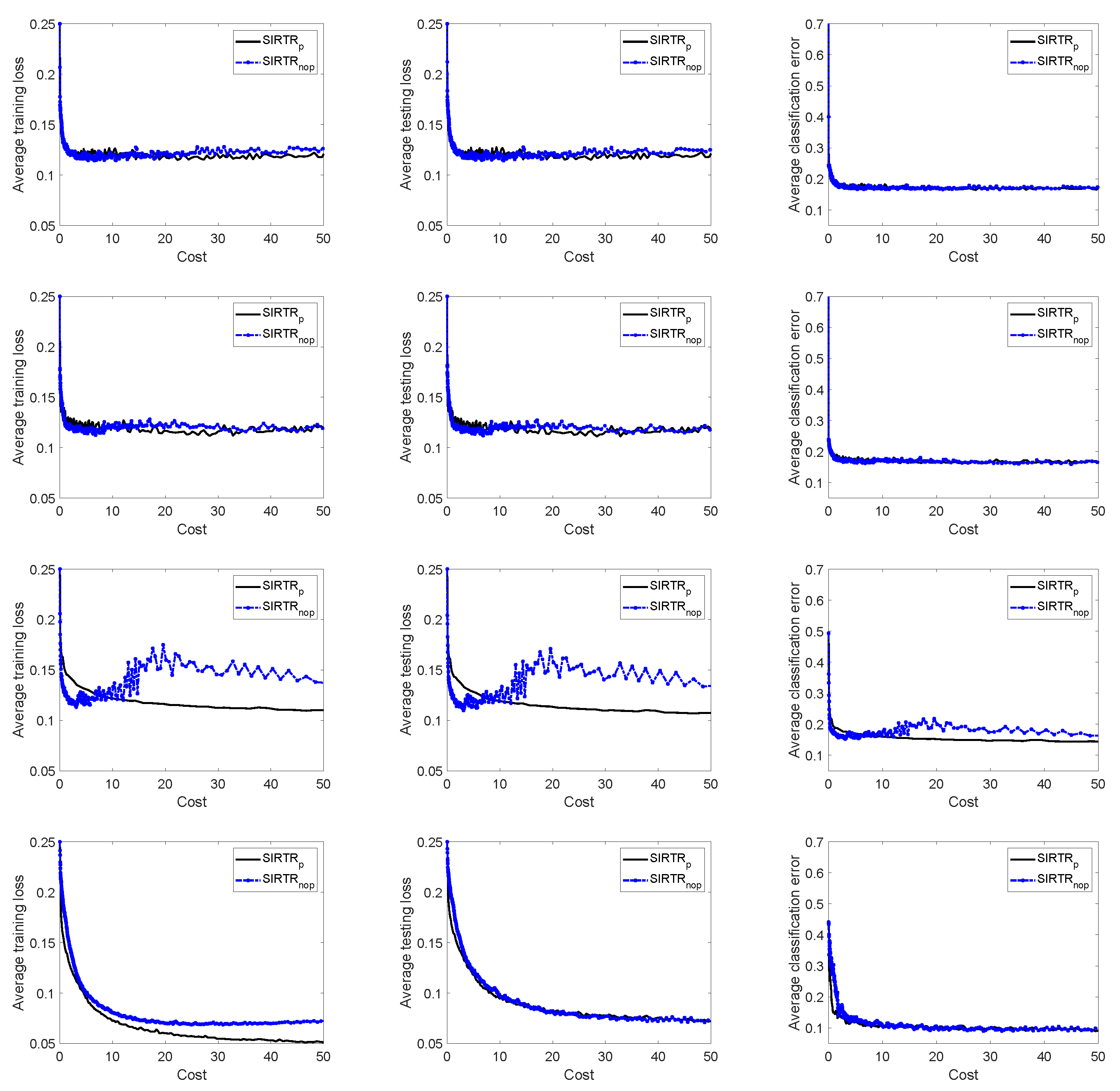
In Figure 1, we show the decrease in the training loss, testing loss, and classification error (all averaged over the 10 runs) versus the average computational cost for the first 20 propagations. For most data sets, we observe that ${\mathrm{SIRTR}}_{\mathrm{nop}}$ performs comparably or even better than ${\mathrm{SIRTR}}_{\mathrm{p}}$. 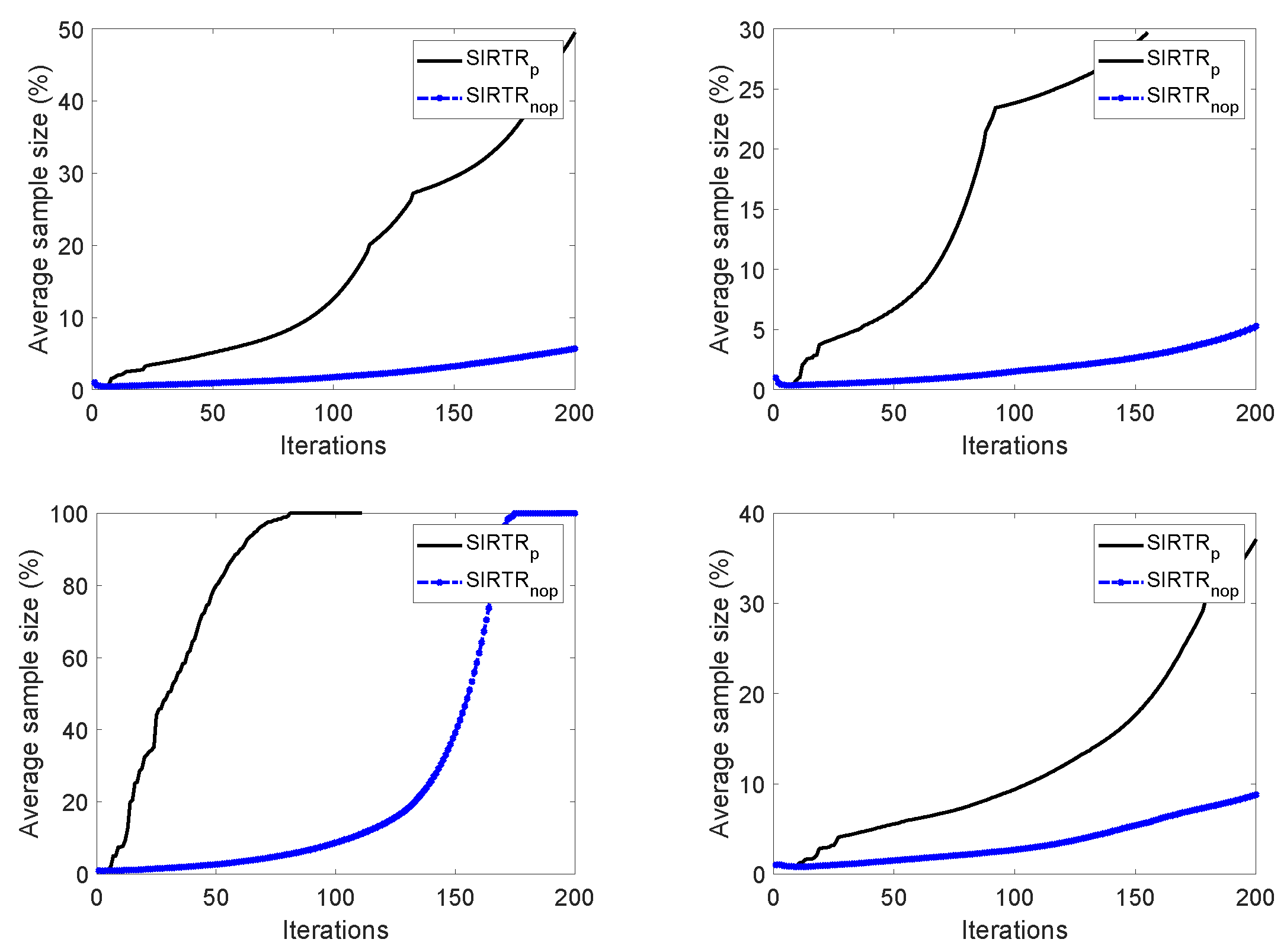However, for one of the four data sets (mnist) in ${\mathrm{SIRTR}}_{\mathrm{nop}}$, the accuracy deteriorates after the first propagations, whereas ${\mathrm{SIRTR}}_{\mathrm{p}}$ provides a more accurate classification and a quite steady decrease in the average training loss, testing loss, and classification error. This different performance of the two algorithms can be explained by looking at Figure 2, which shows the increase in the percentage ratio $\frac{100N_{k+1}}{N}$ of the sample size $N_{k+1}$ over the data set size N (averaged over the 10 runs) for both algorithms. As we can see, the sample size in ${\mathrm{SIRTR}}_{\mathrm{p}}$ rapidly increases to $60\%$ of the data set size in the first 50 iterations, whereas the same percentage is achieved by ${\mathrm{SIRTR}}_{\mathrm{nop}}$ after 150–200 iterations. Overall, we can conclude that the probabilistic requirements of Assumption 4 ensure the theoretical support for convergence in probability but might be excessively demanding. In fact, the numerical examples show that a slower increase in the sample size than that imposed by the probabilistic requirements of Assumption 4 provides a good trade-off between the computational cost and the accuracy in the classification.

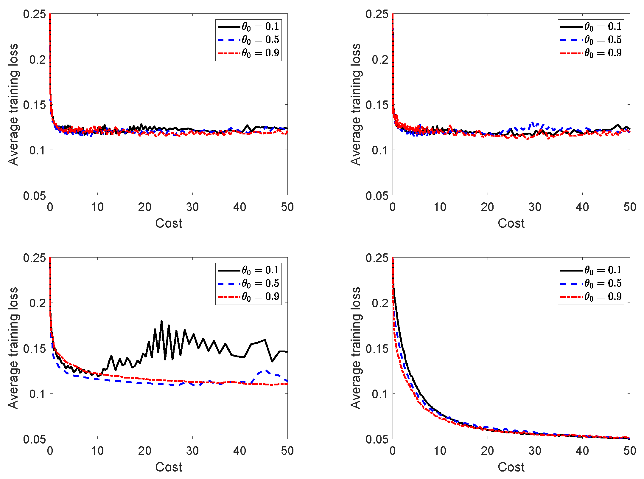
In Figure 3, we test the sensitivity of ${\mathrm{SIRTR}}_{\mathrm{p}}$ with respect to the initial penalty parameter ${\theta }_0$ by reporting the average training loss versus the average computational cost obtained with three different values of ${\theta }_0$. We observe that the performance of the algorithm is not considerably affected by the choice of this parameter, although large oscillations in the average training loss occur for smaller values of ${\theta }_0$ in mnist when ${\theta }_0=0.1$. As a general comment, small initial values of ${\theta }_0$ may not be convenient, as the sequence $\left\{{\theta }_k\right\}$ is non-increasing and small values of ${\theta }_k$ promote a decrease in the infeasibility measure h rather than a decrease in the training loss (see the definition of the actual reduction in (13)). Similar considerations can be made for ${\mathrm{SIRTR}}_{\mathrm{nop}}$ in Figure 4.

5. Conclusions

In this paper, we have proved the convergence in probability of a stochastic trust-region method based on the inexact restoration approach (SIRTR) under the assumption that the function and gradient estimates are sufficiently accurate with sufficiently high probability. This result is novel for SIRTR and agrees with other results obtained in the existing literature [16,18,19]. The numerical experiments on binary classification show that the probabilistic requirements improve the numerical stability of the algorithm, ensuring satisfactory accuracy for all data sets. Future work could address the replacement of the probabilistic requirements considered here with alternative strategies for ensuring convergence in probability, such as variance reduction techniques, or the development of a second-order version of SIRTR for improving accuracy based on approximations of the Hessian obtained through subsampling.