Article

CT-Integral on Interval-Valued Sugeno Probability Measure and Its Application in Multi-Criteria Decision-Making Problems

College of Mathematics and Statistics, Northwest Normal University, Lanzhou 730070, China
*
Authors to whom correspondence should be addressed.
Axioms 2022, 11(7), 317; https://doi.org/10.3390/axioms11070317
Submission received: 16 April 2022 / Revised: 23 June 2022 / Accepted: 24 June 2022 / Published: 29 June 2022

Abstract

:
It is well known that the complexity of the decision-making environment frequently coexists with the diversity of linguistic information in the decision-making process. In order to solve this kind of uncertain multi-criteria decision-making problem, reasonable measures and integrals should be established. In this paper, the discrete expression of the C T -integral on the interval-valued Sugeno probability measure is proposed. The C T -integral is the Choquet integral when the t-norm is T ( x , y ) = x y in the C T -integral and is a pre-aggregation function. Then, the C T -integral on interval-valued Sugeno probability measure is applied to solve end-of-life (EOL) strategy in order to determine multi-criteria decision-making problems. Compared with the general Choquet integral, the method proposed in this paper significantly improves the calculation process, that is, the calculation is simpler and the amount of calculation is smaller. A case study was performed in order to validate the effectiveness of this conclusion.

1. Introduction

In 1954, the French mathematician Choquet introduced capacity theory [1], which is a set function satisfying monotonicity and continuity similar to the Sugeno measure, along with the Choquet integral, which is based on capacity. The Choquet integral is a non-additive measure as well as a nonlinear integral. Afterwards, generalizations of the Choquet integral started to appear; with the work of Sugeno and Murofushi in 1987, a generalized form of the Choquet integral appeared in the literature [2], followed by a corresponding work by Mesiar and Grabisch in 1995. Several other important methods are provided in the literature [3,4], and several boundary conditions have been discussed as well. In 2013, Barrenechea et al. applied the Choquet integral as an aggregation function in a fuzzy rule-based classification system [5]. Then, in 2016, new Choquet integral extensions of the aggregation function appeared in the literature, especially in the research of Lucca et al. [6]. These extensions of the Choquet integral were named, for example, the C C -integral [7], C F -integral [8], and C T -integral [9]. For the C T -integral, the methodology used in these generalizations is simply to replace the product in the Choquet integral, which can be interpreted as the product’s t-norm, with other fusion functions with appropriate properties in order to obtain a resulting aggregation-type function.
The Choquet integral is applied in many fields, such as risk evaluation [10], fuzzy systems and control [11], decision-making, and more (see [12,13,14,15]). For the multi-attribute decision-making problem ([12,16]), the multi-criteria decision-making problem [15], and the group decision-making problem [13], it can be used as aggregation operators to aggregate. Similarly, the C T -integral can be applied to multi-criteria decision-making problems; see [17]. Other generalizations of the Choquet integral have seen use in problems involving multi-criteria decision-making (see [18,19]). In this paper, we focus on multi-criteria decision-making problems. Especially in the multi-criteria decision-making problem of end-of-life (EOL) strategy, the Choquet integral is used as an aggregation operator to aggregate data. However, with the emergence of the generalization of the Choquet integral, generalization solves this type of problem more efficiently than the Choquet integral.
With the development of society and the progress of science and technology, more and more people have begun to pay attention to the EOL strategy of products and how to deal with product after use. Many definitions and classifications of EOL strategy have been developed over the decades. EOL strategy has been continuously developed and improved following its initial proposal by Marco et al. in 1994 [20]. The detailed development process of EOL strategies can be followed in the literature [21]. For a product, EOL strategy analysis is more beneficial to the development of both the environment and the economy. Moreover, certain EOL strategies produce a large amount of energy waste, environmental pollution, and cost over the whole product life cycle. Therefore, the theory and method of EOL research has been a concern of many scholars. EOL decision-making depends on many factors which arise from a wide range of stakeholder interests and components, and the view of the results varies by industry and geographical location. As far as we know, the EOL strategy of refrigerator components is an important research area in evaluating EOL decision factors from a comprehensive perspective. Therefore, it is meaningful to use our proposed C T -integral on interval-valued Sugeno probability measure to solve related uncertain multi-criteria decision-making problems in this paper.
When we solving this kind of multi-criteria decision-making problems, the decision criteria usually interact with each other, and the evaluation values are usually fuzzy linguistic evaluations by experts, often defined as “good”, “a little good” etc. These linguistic calculations are usually converted into triangular fuzzy numbers for calculation; however, triangular fuzzy numbers are not easy to calculate. Generally, they are converted into interval values or exact values for operation. Therefore, it is necessary to extend the general C T -integral to the interval value. In 2016, a new aggregation-like function generalizing the Choquet integral was proposed in [22]. In 2020, Chen et al. proposed the Choquet integral on the interval-valued Sugeno probability measure [23]. The discrete expression of the C T -integral on the interval-valued Sugeno probability measure is proposed in this paper and applied to solve multi-criteria decision-making problems in the context of determining EOL strategy.
It is well known that in dealing with uncertain multi-criteria decision-making problems, the decision criteria usually interact with each other. The Choquet integral on fuzzy measures based on σ - λ rules can be used to solve such problems effectively. The discrete expression of the C T -integral on the interval-valued Sugeno probability measure is proposed in this paper. The C T -integral is the Choquet integral when the t-norm is T ( x , y ) = x y in the C T -integral and is a pre-aggregation function. Then, we apply the C T -integral on interval-valued Sugeno probability measure to determine end-of-life (EOL) strategy as a multi-criteria decision-making problems. Compared with the general Choquet integral, the method proposed in this paper significantly improves the calculation process, that is, the calculation is simpler and the amount of calculation required is smaller. A case study is performed in order to validate the effectiveness of the conclusions.
The remainder of the article is organized as follows. In Section 2, several basic concepts are introduced. Section 3 provides the C T -integral on the interval-valued Sugeno probability measure. In Section 4, a multi-criteria decision-making problem involving the EOL strategy for a refrigerator component is illustrated as a case study. Our conclusions are presented in Section 5.

2. Preliminaries

In this section, basic concepts are introduced. In the following, n > 0 , Ω is a non-empty set, and A is a σ -algebra.
Definition 1
([24]). The fuzzy measure μ is a set function
μ : A [ 0 , ]
with the following properties:
(i)
μ ( ) = 0 ;
(ii)
A B implies μ ( A ) μ ( B ) ;
Fuzzy measure μ is said to be lower semi-continuous when it satisfies
(iii)
A 1 A 2 . . . , implying that μ ( n = 1 A n ) = lim n 0 μ ( A n ) ;
Fuzzy measure μ is said to be upper semi-continuous when it satisfies
(iv)
A 1 A 2 . . . , and μ ( A 1 ) < , implying that μ ( n = 1 A n ) = lim n 0 μ ( A n ) ;
Fuzzy measure μ is said to be continuous if it satisfies both lower semi-continuity and upper semi-continuity.
Definition 2
([25]). Consider function T : [ 0 , 1 ] 2 [ 0 , 1 ] . Then, T is the triangular norm (t-norm for short) if, for all x , y , z [ 0 , 1 ] , the following four axioms are satisfied:
(T1)
Commutativity: T ( x , y ) = T ( y , x ) ;
(T2)
Associativity: T ( x , T ( y , z ) ) = T ( T ( x , y ) , z ) ;
(T3)
Monotonicity: T ( x , y ) T ( x , z ) whenever y z ;
(T4)
Boundary condition: T ( x , 1 ) = x .
The basic definitions of the interval-valued Sugeno probability measure (see [23]) are provided below; R + denotes [ 0 , ) .
Definition 3
([23]). Suppose Ω is a nonempty set and A is σ-algebra on the Ω. The set function μ is a fuzzy measure based on σ-λ rules if
μ i = 1 A ( i ) = 1 λ Π i = 1 1 + λ μ ( A ( i ) ) 1 λ 0 , i = 1 μ A ( i ) λ = 0 .
where λ 1 s u p μ , 0 , A ( i ) A , A ( i ) A ( j ) = for all i , j = 1 , 2 . . . , and i j .
Definition 4
([23]). Suppose Ω is a nonempty set and A a σ-algebra on the Ω, a set function μ : A R + , μ ̲ : A R + , μ ¯ : A R + , μ ̲ and μ ¯ satisfying the following conditions:
(1) 
μ ̲ ( ) = 0 , μ ¯ ( ) = 0 ;
(2) 
if A , B Ω , and A B , then μ ̲ ( A ) μ ̲ ( B ) , μ ¯ ( A ) μ ¯ ( B ) ;
(3) 
for every A Ω , μ ̲ ( A ) μ ¯ ( A ) ;
then μ = [ μ ̲ , μ ¯ ] is an interval-valued fuzzy measure.
Definition 5
([23]). If μ ̲ and μ ¯ satisfy the σ λ rules in (Definition 3), and μ ̲ ( Ω ) = 1 , μ ¯ ( Ω ) = 1 , then μ = [ μ ̲ , μ ¯ ] is called an interval-valued Sugeno probability measure based on σ λ rules, or simply an interval-valued Sugeno probability measures, and denoted g λ = [ g ̲ λ , g ¯ λ ] .
L ( 0 , 1 ) denotes the set of all closed subintervals of the unit interval.
Definition 6
([23]). Suppose Ω is a finite set and 2 Ω is the power set of Ω, the set function μ: 2 Ω [ μ ̲ , μ ¯ ] L ( 0 , 1 ) is a regular interval fuzzy measure defined on 2 Ω if the following conditions hold:
(1) 
μ ̲ ( ) = 0 , μ ¯ ( ) = 0 , μ ̲ ( Ω ) = 1 , μ ¯ ( Ω ) = 1 ;
(2) 
if D 2 Ω , H 2 Ω , D H , then μ ̲ ( D ) μ ̲ ( H ) , μ ¯ ( D ) μ ¯ ( H ) .
Definition 7
([23]). Suppose Ω is a finite set and 2 Ω is the power set of Ω; set function μ: 2 Ω [ μ ̲ , μ ¯ ] L ( 0 , 1 ) , is a regular λ —interval fuzzy measure defined on 2 Ω if the following conditions hold:
(1) 
μ ̲ ( ) = 0 , μ ¯ ( ) = 0 , μ ̲ ( Ω ) = 1 , μ ¯ ( Ω ) = 1 ;
(2) 
if A Ω , B Ω , A B = , then
μ ̲ ( A B ) = μ ̲ ( A ) + μ ̲ ( B ) + λ μ ̲ ( A ) μ ̲ ( B ) ,
and
μ ¯ ( A B ) = μ ¯ ( A ) + μ ¯ ( B ) + λ μ ¯ ( A ) μ ¯ ( B ) , λ ( 1 , ) .
Theorem 1
([23]). If g λ = [ g ̲ λ , g ¯ λ ] is an interval-valued Sugeno probability measure, then g λ is a regular λ —interval fuzzy measure defined on A .
Proof. 
Refer to the proof of Theorem 3.1.2 in [23]. □
Suppose X = { x 1 , x 2 , . . . , x n } is a finite set. Then, g λ i = g λ ( x i ) ( i = 1 , 2 , . . . , n ) can measure the density.
Theorem 2
([24,26]). The parameters λ = ( λ 1 , λ 2 ) of the regular interval Sugeno probability measure are determined by the following equations:
i = 1 n 1 + λ 1 g ̲ λ i = 1 + λ 1 ,
i = 1 n 1 + λ 2 g ¯ λ i = 1 + λ 2 .
Proof. 
Because Theorem 1 and λ = ( λ 1 , λ 2 ) take into account that X = { x 1 , x 2 , . . . , x n } is a finite set, g λ i = g λ ( x i ) ( i = 1 , 2 , . . . , n ) is said to be a measure of density. From Equation (1) λ 0 , have g λ i i = 1 n ( x i ) = 1 , that is,
1 λ i = 1 n 1 + λ 1 g λ i ( x ( i ) ) 1 = 1 ,
i = 1 n 1 + λ 1 g ̲ λ i ( x ( i ) ) 1 = λ 1 ,
i = 1 n 1 + λ 1 g ̲ λ i ( x ( i ) ) = 1 + λ 1 ,
i.e.,
i = 1 n 1 + λ 1 g ̲ λ i = 1 + λ 1 .
Then, Equation (5) can be obtained similarly.

3. The CT-Integral on Interval-Valued Sugeno Probability Measure

Choquet integrals are a natural generalization of the Lebesgue integral; the definition of Lebesgue integrals considers additive measures, whereas the definition of Choquet integrals considers fuzzy measures. In the following, the definition of the discrete Choquet integral is introduced and the discrete expression of the C T -integral on the interval-valued Sugeno probability measure is proposed. Consider N = { 1 , . . . , n } as a finite set.
Definition 8
([1]). Suppose m : 2 N [ 0 , 1 ] is a fuzzy measure; then, the discrete Choquet integral as regards m is the function C m : [ 0 , 1 ] n [ 0 , 1 ] , defined for all x = ( x 1 , . . . , x n ) [ 0 , 1 ] n by
C m x = i = 1 n x ( i ) x ( i 1 ) · m A ( i ) ,
where x ( 1 ) , . . . , x ( n ) is an increasing permutation on the input x , that is, x ( 1 ) . . . x ( n ) , with the convention that x ( 0 ) = 0 and A ( i ) = { i , . . . , n } is the subset of indices corresponding to the n i + 1 largest components of x .
Reference [9] mentions recent advances in the generalization of the standard form of the Choquet integral. The method used for these generalizations is simple, and allows for replacing the product operator in Equation (6) with another fusion function of a suitable nature. The C T -integral is obtained by replacing the product operator of Equation (6) with a t-norm, and is a pre-aggregation function.
Definition 9
([9]). Suppose m: 2 N [ 0 , 1 ] is a fuzzy measure and T : [ 0 , 1 ] 2 [ 0 , 1 ] is a t-norm. Based on the Choquet integral, the C T -integral is defined as the function C m T : [ 0 , 1 ] n [ 0 , 1 ] for all of x = ( x 1 , . . . , x n ) [ 0 , 1 ] n by
C m T x = i = 1 n T x ( i ) x ( i 1 ) , m ( A ( i ) ) ,
where:
(1) 
x ( 1 ) , . . . , x ( n ) is an increasing permutation on the input x , that is, x ( 1 ) . . . x ( n ) ;
(2) 
x ( 0 ) = 0 ;
(3) 
A ( i ) = { ( i ) , . . . , ( n ) } is the subset of indices corresponding to the n i + 1 largest component of x .
The C T -integral has the averaging and idempotent properties after generalization, as shown below.
Proposition 1
([6,8]). Let T : [ 0 , 1 ] 2 [ 0 , 1 ] be a t-norm such that T ( x , y ) x for every x , y [ 0 , 1 ] . Then,
C m T ( x 1 , . . . , x n ) max ( x 1 , . . . , x n ) ,
for every ( x 1 , . . . , x n ) [ 0 , 1 ] n .
Proposition 2
([6,8]). Let T : [ 0 , 1 ] 2 [ 0 , 1 ] be a t-norm such that T ( x , 1 ) = x for every x , y [ 0 , 1 ] . Then,
C m T x 1 , . . . , x n min x 1 , . . . , x n ,
for every ( x 1 , . . . , x n ) [ 0 , 1 ] n .
Proposition 3
([6,8]). Let T : [ 0 , 1 ] 2 [ 0 , 1 ] be a t-norm such that T ( x , 1 ) = x and T ( 0 , y ) = 0 for every x , y [ 0 , 1 ] . Then, C m T is an idempotent function, that is,
C m T ( x , . . . , x ) = x .
Next, the measurability and integrability of interval-valued functions is introduced.
R + = [ 0 , ) , I ( R + ) = r : [ r ̲ , r ¯ ] R + is the subset of the interval number, while P 0 ( R + ) denotes the classes of all non-empty subsets on R + .
Definition 10
([27]). Suppose ( Ω , A , μ ) is a non-additive measure space and F : Ω I ( R + ) is a non-negative measurable interval-valued function on Ω, A A ; then, we have
( c ) A F d μ = ( c ) A f d μ : f S F ,
where S F = g | g : Ω R + is a measurable selection on F ; if ( c ) A F d μ I ( R + ) , then F is C-integrable.
Definition 11
([27]). F is C-integrally bounded if there exists a C-integral function g : Ω P 0 ( R + ) such that for any measurable selection f S F , A A has
( c ) A f d μ ( c ) A g d μ .
Theorem 3
([23]). Let ( Ω , A , μ ) be a non-additive measure space, μ be a fuzzy measure, A A , F be non-negative measurable, and C —be integrally bounded; then, F is C —integrable on A and
( c ) A F d μ = ( c ) A F ̲ d μ , ( c ) A F ¯ d μ .
Proof. 
See [23] in Theorem 3.2.1. □
We know from the previous that the interval-valued function f is C-integrable on A if ( c ) A f ̲ d μ and ( c ) A f ¯ d μ exists and is bounded.
Suppose X = { x 1 , x 2 , . . . x n } is a discrete set; we can then obtain the following Theorem.
Theorem 4.
Suppose f is an interval-valued function on X = { x 1 , x 2 , . . . x n } and T is a t-norm. Then, the C T -integral of f as regards the interval-valued Sugeno probability measure g λ on X is provided by
( c ) X f d g λ = i = 1 n T g λ X i g λ X i + 1 , f X i ,
where x 1 , x 2 , . . . , x n is a permutation of x 1 , x 2 , . . . , x n such that f ( x 0 ) f ( x 1 ) . . . f ( x n ) , f ( x 0 ) = [ 0 , 0 ] , X i = { x i , x i + 1 , . . . , x n } , i = 1 , 2 , . . . , n , and X n + 1 = .
Proof. 
Due to f being an interval-valued function on X, per Theorem 3, we have
( c ) X f d g λ = ( c ) X f ̲ d g λ , ( c ) X f ¯ d g λ .
Note that f ̲ and f ¯ are real-valued functions on X, respectively, on account of the continuity and monotonicity of the C T -integral. Meanwhile, considering the nonnegativity and the monotonicity of the fuzzy measure, we can obtain
( c ) X f d g λ = i = 1 n T g λ X i g λ X i + 1 , f ̲ X i , i = 1 n T g λ X i g λ X i + 1 , f ¯ X i = i = 1 n T g λ X i g λ X i + 1 , f ̲ X i , T g λ X i g λ X i + 1 , f ¯ X i = i = 1 n T g λ X i g λ X i + 1 , f ̲ X i , f ¯ X i = i = 1 n T g λ X i g λ X i + 1 , f X i .
where x 1 , x 2 , . . . , x n is a permutation of x 1 , x 2 , . . . , x n such that f ( x 0 ) f ( x 1 ) . . . f ( x n ) , f ( x 0 ) = [ 0 , 0 ] , X i = { x i , x i + 1 , . . . , x n } , i = 1 , 2 , . . . , n , and X n + 1 = .
Then, the discrete representation of the C T -integral on interval-valued Sugeno probability measure is as follows:
( c ) X f d g λ = i = 1 n T g λ X i g λ X i + 1 , f ̲ X i , i = 1 n T g λ X i g λ X i + 1 , f ¯ X i .
where T can be T M , T P , T , T D P , T N M , and T H P . When T is T M , T M ( x , y ) = min { x , y } , we have an expression of the C T M -integral on interval-valued Sugeno probability measure:
( c ) X f d g λ = i = 1 n min g λ X i g λ X i + 1 , f X i = i = 1 n min g λ X i g λ X i + 1 , f ̲ X i , f ¯ X i = i = 1 n min g λ X i g λ X i + 1 , f ̲ X i , min g λ X i g λ X i + 1 , f ¯ X i = i = 1 n min g λ X i g λ X i + 1 , f ̲ X i , i = 1 n min g λ X i g λ X i + 1 , f ¯ X i .

4. Application in Multi-Criteria Decision-Making Problems

4.1. Case Study

In this case, the multi-criteria decision-making problem of EOL strategy determination for a refrigerator component was studied. We used the extended form of the Choquet integral, which is the C T -integral. This multi-criteria decision-making problem considers four primary criteria and fourteen sub-criteria, as shown in Figure 1. Each component of the refrigerator interacts with other components, and includes only the main part and a few small connectors. The case data sets are taken from [21,28]. The decision alternatives include reuse, restructuring, primary recycling, secondary recycling, refuse incineration, and landfill.
In [12], the language assessment and every attribute are represented by triangular fuzzy numbers. We can evaluate this in natural language and turn it into a triangular fuzzy number. Such an evaluation process requires the participation of participating decision-makers. The language assessment and corresponding triangular fuzzy numbers are provided in Table 1. As an example of the cabinet frame, Table 2 shows the language evaluation of the main criteria and subcriteria, while Table 3 shows the corresponding triangular fuzzy numbers.

4.2. Case Studies and Solutions

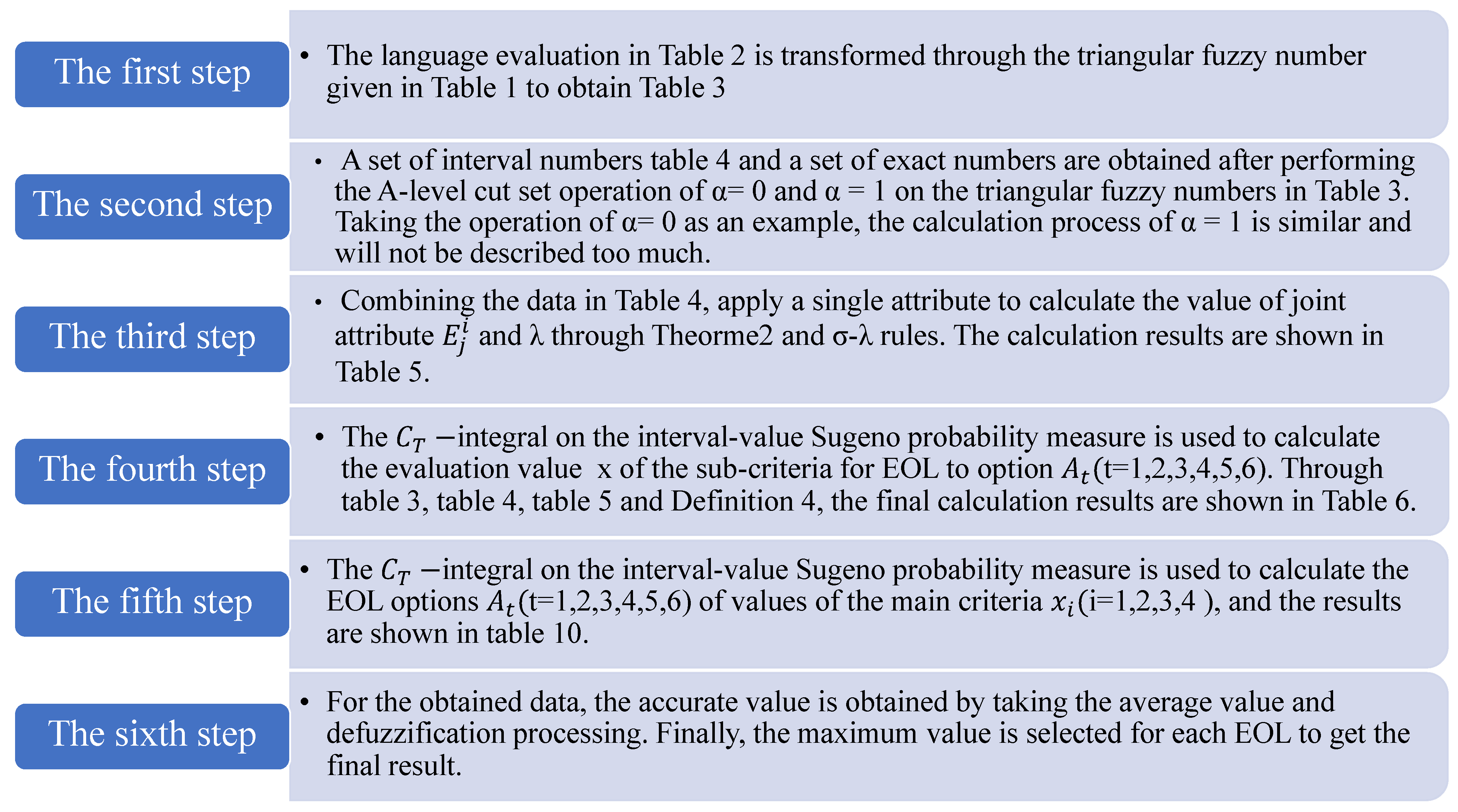
The calculation process for the refrigerator component EOL strategy determination multi-criteria decision-making problem is as follows, in the six steps shown in Figure 2. 
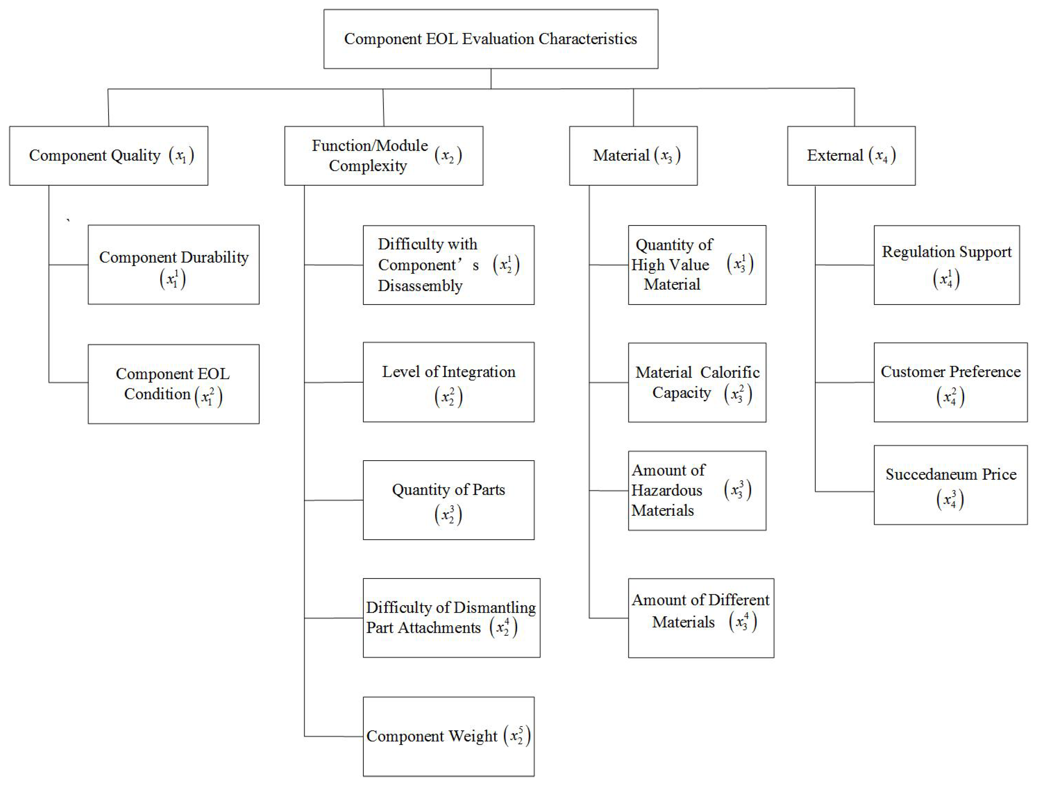
Figure 1 describes the parameter set and variables. In this example, four primary criteria are considered, denoted as x i ( i = 1 , 2 , 3 , 4 ) , and fourteen sub-criteria, denoted as x i j . If i = 1 , then j = 1 , 2 , if i = 2 , then j = 1 , 2 , 3 , 4 , 5 , if i = 3 , then j = 1 , 2 , 3 , 4 , and if i = 4 then j = 1 , 2 , 3 . The six EOL choices (Reuse, Remanufacture, Primary Recycling, Secondary Recycling, Incineration, and Landfill) are A 1 , A 2 , A 3 , A 4 , A 5 , and A 6 , respectively.
Taking α = 0 as an example, α = 1 analogies can be obtained.
The evaluated language information is transformed into triangular fuzzy numbers; Table 2 shows the criteria weights and the linguistic assessment of each EOL strategy. According to Table 1 these can be obtained from the experiment, and Table 3 indicates the corresponding linguistic assessment of the triangular fuzzy numbers.
Second Step: an α -level cut set operation performed on the triangular fuzzy numbers in Table 3 and Table 4 are the operation results of α = 0 ; α = 1 can be obtained similarly.
Third Step: Combining the data in Table 4, we apply a single attribute to calculate the value of the joint attributes E i j and λ through Theorem 2 and σ λ rules. The calculation results are shown in Table 5; E i j = { x i j , x i j + 1 , . . . , x i n } . If i = 1 , then n = 2 , if i = 2 , then n = 5 , if i = 3 , then n = 4 , and if i = 4 , then n = 3 , 1 j n . Furthermore, g ̲ λ ( j ) = g ̲ λ ( E i j ) , g ¯ λ ( j ) = g ¯ λ ( E i j ) .
Fourth Step: calculate the evaluation value of the sub-criteria x j i regarding the EOL options A t ( t = 1 , 2 , 3 , 4 , 5 , 6 ) . According to the third step, we know that ( f i , t j ) α stands for the function f i , t j α -level cut set, while ( f i , t j ) 0 stands for the 0-level cut set of function f i , t j .
For EOL options A 1 about criteria x 2 , α = 0 .
(1)
From Table 4, we can obtain ( f 2 , 1 1 ) 0 = [ 0.7 , 0.9 ] , ( f 2 , 1 2 ) 0 = [ 0.8 , 1 ] , ( f 2 , 1 3 ) 0 = [ 0.4 , 0.6 ] , ( f 2 , 1 4 ) 0 = [ 0.4 , 0.6 ] , ( f 2 , 1 5 ) 0 = [ 0.7 , 0.9 ] .
(2)
From Table 4, we can obtain ( g λ ) 2 1 = [ 0.7 , 0.9 ] , ( g λ ) 2 2 = [ 0.4 , 0.6 ] , ( g λ ) 2 3 = [ 0.7 , 0.9 ] , ( g λ ) 2 4 = [ 0.8 , 1 ] , ( g λ ) 2 5 = [ 0.4 , 0.6 ] .
(3)
From Definition 4, f ̲ i , t j and f ¯ i , t j stand for the left and right endpoints of the α -level cut set of the function f i , t j respectively. In order of magnitude f ̲ i , t j , we have f ̲ 2 , 1 3 f ̲ 2 , 1 4 f ̲ 2 , 1 1 f ̲ 2 , 1 5 f ̲ 2 , 1 2 . Then, we have x 2 1 , x 2 2 , x 2 3 , x 2 4 , x 2 5 , which is a permutation of x 2 1 , x 2 2 , x 2 3 , x 2 4 , x 2 5 ; then, x 2 1 = x 2 3 , x 2 2 = x 2 4 , x 2 3 = x 2 1 , x 2 4 = x 2 5 , x 2 5 = x 2 2 .
The value of parameter λ 1 is calculated using Theorem 2, that is λ 1 = 0.993 . Furthermore, we can calculate the weight of the joint attribute according to σ - λ rules and obtain their values as g ̲ λ ( j ) = g ̲ λ ( E i j ) = g ̲ λ { x i j , x i ( j + 1 ) , . . . , x i n } ,
g ̲ λ ( 5 ) = 0.4 , g ̲ λ ( 4 ) = 0.641 , g ̲ λ ( 3 ) = 0.896 , g ̲ λ ( 2 ) = 0.984 , g ̲ λ ( 1 ) = 1 .
Table 5 lists all measured values and the values of the required parameters λ .
(4)
The value of the main criteria ( x i , i = 1 , 2 , 3 , 4 ) ) regarding the EOL options A t ( t = 1 , 2 , 3 , 4 , 5 ) are calculated using the C T -integral as follows; taking “primary criteria x 2 of EOL options A 1 ”, for example, α = 0 :
( c ) f ̲ 2 , 1 j d g ̲ λ = min { f ̲ 2 , 1 3 , g ̲ λ ( 1 ) } + min { f ̲ 2 , 1 4 f ̲ 2 , 1 3 , g ̲ λ ( 2 ) } + min { f ̲ 2 , 1 1 f ̲ 2 , 1 4 , g ̲ λ ( 3 ) } + min { f ̲ 2 , 1 5 f ̲ 2 , 1 1 , g ̲ λ ( 4 ) } + min { f ̲ 2 , 1 2 f ̲ 2 , 1 5 , g ̲ λ ( 5 ) } = min 0.4 0 , 1 + min { 0.4 0.4 , 0.972 } + min { 0.7 0.4 , 0.896 } + min { 0.7 0.7 , 0.641 } + min { 0.8 0.7 , 0.4 } = 0.4 + 0 + 0.3 + 0 + 0.1 = 0.8 .
In the same manner, ( c ) f ¯ 2 , 1 j d g ¯ λ = 1 . Therefore,
( c ) f 2 , 1 j d g ̲ λ = ( c ) f ̲ 2 , 1 j d g ̲ λ , ( c ) f ¯ 2 , 1 j d g ¯ λ = [ 0.8 , 1 ] .
Similarly, we can calculate the evaluation values for the remaining sub-criteria, as shown in Table 6.
Fifth Step: The C T -integral on the interval-value Sugeno probability measure is used to calculate the EOL options ( A 1 , A 2 , A 3 , A 4 , A 5 , A 6 ) of the values of the main criteria, x i ( i = 1 , 2 , 3 , 4 ) .
For EOL option A 1 , α = 0 ; then,
(1)
From Table 6, we can obtain ( f 1 , 1 ) 0 = [ 0.7 , 0.9 ] , ( f 2 , 1 ) 0 = [ 0.8 , 1 ] , ( f 3 , 1 ) 0 = [ 0.8 , 1 ] , ( f 4 , 1 ) 0 = [ 0.8 , 1 ] .
(2)
From Table 6, we can obtain g λ ( x 1 ) = [ 0.8 , 1 ] , g λ ( x 2 ) = [ 0.7 , 0.9 ] , g λ ( x 3 ) = [ 0.8 , 1 ] , g λ ( x 4 ) = [ 0.4 , 0.6 ] .
(3)
In order of magnitude f ̲ i , 1 , f ̲ i , 1 ( i = 1 , 2 , 3 , 4 ) , there are f ̲ 1 , 1 f ̲ 2 , 1 f ̲ 3 , 1 f ̲ 4 , 1 . Then, we have x 1 , x 2 , x 3 , x 4 , which is a permutation of x 2 1 , x 2 2 , x 2 3 , x 2 4 , where x 1 = x 1 , x 2 = x 2 , x 3 = x 3 , x 4 = x 4 .
Then, the values of the parameters λ and the weights of the joint attributes on the main criterion were calculated in the same way. These are listed in Table 7.
(4)
For the EOL options, A t ( t = 1 , 2 , 3 , 4 , 5 , 6 ) are calculated using the C T -integral as follows:
( c ) f ̲ i , 1 d g ̲ λ = min { f ̲ 2 , 1 , g ̲ λ ( 1 ) } + min { f ̲ 2 , 1 f ̲ 2 , 1 , g ̲ λ ( 2 ) } + min { f ̲ 2 , 1 f ̲ 2 , 1 , g ̲ λ ( 3 ) } + min { f ̲ 2 , 1 f ̲ 2 , 1 , g ̲ λ ( 4 ) } + min { f ̲ 2 , 1 f ̲ 2 , 1 , g ̲ λ ( 5 ) } = min { 0.4 0 , 1 } + min { 0.4 0.4 , 0.972 } + min { 0.7 0.4 , 0.896 } + min { 0.7 0.7 , 0.641 } + min { 0.8 0.7 , 0.4 } = 0.4 + 0 + 0.3 + 0 + 0.1 = 0.8 .
In the same way, ( c ) f ¯ i , 1 d g ¯ λ = 1 . Therefore,
( c ) f 2 , 1 d g ̲ λ = ( c ) f ̲ 2 , 1 d g ̲ λ , ( c ) f ¯ 2 , 1 d g ¯ λ = [ 0.8 , 1 ] .
Similarly, it is possible to calculate the evaluation values for the remaining primary criteria, as shown in Table 8.
Sixth Step: In the process of fuzzy number processing, as the triangular fuzzy numbers cannot be applied directly we must first defuzzify the fuzzy numbers before applying them. There are many methods of defuzzification, and in this study, we choose the mean value method of defuzzification. The mean value was calculated for each of the triangular fuzzy numbers in Table 8 in order to convert the fuzzy number into an exact number.
A similar optimal EOL option for other the components can be obtained as shown in Table 9.
For data comparison, in Table 1, Table 2, Table 3, Table 4 and Table 5 and Table 10, Table 11 and Table 12 we use the data in [23], while Table 6, Table 8 and Table 9 show the results obtained in this paper. Although the final EOL strategy standards reached by the two are the same, the final data obtained are different. Compared with [23], the data with the method in this paper are more concise.
In the above example, we know that Table 10 shows the result of the sub-criteria for the general Choquet aggregation and Table 6 the result of the sub-criteria for the aggregation of C T M -integral. Table 11 and Table 12 contain the final results of the aggregation of the general Choquet integral, while Table 8 and Table 9 are the final results of the aggregation of C T M -integral. By comparing them, we know that the same result as the general Choquet integral can be obtained when the t-norm in the C T integral is taken as the minimum t-norm ( T M ). In this case, the C T integral is more advantageous than the Choquet integral in terms of calculation efficiency.

5. Conclusions

Through the derivation process and examples provided in the paper, we find that the C T -integral on the interval-valued Sugeno probability measure is more advantageous than the general Choquet integral on the interval-valued Sugeno probability measure. Moreover, the C T -integral on interval-valued Sugeno probability measure improves the computational procedure, making the computation simpler and less intensive compared to the general Choquet integral on interval-valued Sugeno probability measure. Furthermore, the C T -integral is the Choquet integral when the t-norm is T ( x , y ) = x y in the C T -integral. In addition, this paper only provides the discrete expression of the C T -integral on the interval-valued Sugeno probability measure, in particular its application in multi-criteria decision-making problems; its specific properties are not studied, nor are its properties as a pre-aggregation function. These properties of the C T -integral should be considered in future work in order to obtain a better understand of the C T -integral and its potential applications.
Although this paper studies C T -integral, it only studies its applications and characteristics in the context of the interval-valued Sugeno measure. Important research on the C T -integral has yet to be carried out. For example, the C T -integral is more widely applicable than the Choquet integral. The calculation intensity of the C T M -integral o then C T -integral is less than that od the Choquet integral, thus, whether T Ł , T D P , T N M , and T H P are the same as the C T -integral is worth studying in the future.

Author Contributions

H.Y., L.S. and Z.G. completed the main study together. L.S. wrote the manuscript, H.Y. checked the proofs process and verified the calculation. All authors have read and agreed to the published version of the manuscript.

Funding

This work was supported by the Natural Science Foundation of China (No.12161082, No.12061067), the Natural Science Foundation of Gansu Province (No.21JR7RA134), and the University Innovation and Entrepreneurship Fund of Gansu Province (2020A-009).

Data Availability Statement

Data is contained within the article.

Acknowledgments

The authors are very grateful to the anonymous referees.

Conflicts of Interest

The authors declare no conflict of interest.

References

  1. Choquet, G. Theory of capacities. Annales de L’Institute Fourier 1954, 5, 131–295. [Google Scholar] [CrossRef] [Green Version]
  2. Sugeno, M.; Murofushi, T. Pseudo-additive measure and integral. J. Math. Anal. Appl. 1987, 122, 197–222. [Google Scholar] [CrossRef] [Green Version]
  3. Grabisch, M. Fuzzy measure and inregrals: Recent developments. In Fifty Years of Fuzzy Logic and its Applications; Tamir, D.E., Rishe, N.D., Kandel, A., Eds.; Spring International Publishing: Cham, Switzerland, 2015; pp. 9–12. [Google Scholar]
  4. Mesiar, R. Choquet-like integral. J. Math. Anal. Appl. 1995, 194, 477–488. [Google Scholar] [CrossRef]
  5. Barrenechea, E.; Bustince, H.; Fernández, J.; Paternain, D.; Sanz, J.A. Using the Choquet integral in the fuzzy reasoning method of fuzzy rule-based classification systems. Axioms 2013, 2, 208–223. [Google Scholar] [CrossRef] [Green Version]
  6. Lucca, G.; Sanz, J.; Dimuro, G.P. Pre-aggregation function: Construction and an application. IEEE Trans. Fuzzy Syst. 2016, 24, 260–272. [Google Scholar] [CrossRef]
  7. Lucca, G.; Sanz, J.A.; Dimuro, G.P.; Bedregal, B.; Asiain, M.J.; Elkano, M.; Bustince, H. CC-integrals: Choquet-like copula-based aggregation functions and its application in fuzzy rule-based classification systems. Knowl.-Based Syst. 2017, 119, 32–43. [Google Scholar] [CrossRef]
  8. Lucca, G.; Sanz, J.A.; Dimuro, G.P.; Bedregal, B.; Bustince, H.; Mesiar, R. CF-integrals: A new family of pre-aggregation functions with application to fuzzy rule-based classification systems. Inf. Sci. 2018, 435, 94–110. [Google Scholar] [CrossRef]
  9. GDimuro, P.; Fernández, J.; Bedregal, B.; Mesiar, R.; Sanz, J.A.; Lucca, G.; Bustince, H. The State-of-Art of the Generalization of the Choquet integral: From aggregation and pre-aggregation to ordered directionally monotone function. Inf. Fusion 2020, 57, 27–43. [Google Scholar] [CrossRef]
  10. Wang, W.; Lin, X.; Qin, Y.; Fu, Y. A risk evaluation and prioritization method for FMEA with prospect theory and Choquet integral. Saf. Sci. 2018, 110, 152–163. [Google Scholar] [CrossRef]
  11. Masoudi, S.; Soltanpour, M.S.; Abdollahi, H. Adaptive fuzzy control method for a linear switched reluctance motor. IET Electr. Power Appl. 2018, 12, 1328–1336. [Google Scholar] [CrossRef]
  12. Chen, S.; Hwang, C.L. Fuzzy Multiple Attribute Decision-Making: Methods and Application; Springer: New York, NY, USA, 1992. [Google Scholar]
  13. Garg, H.; Krishankumar, R.; Ravichandran, K.S. Decision framework with integrated methods for group decision-making under probabilistic hesitant fuzzy context and unknown weights. Expert Syst. Appl. 2022, 200, 117082. [Google Scholar] [CrossRef]
  14. Garg, H. Some methods for strategic decision-making problems with immediate probabilities in Pythagorean fuzzy environment. Int. J. Intell. Syst. 2018, 33, 687–712. [Google Scholar] [CrossRef]
  15. Rani, P.; Govindan, K.; Mishra, A.R.; Mardani, A.; Alrasheedi, M.; Hooda, D.S. Unified Fuzzy Divergence Measures with Multi-Criteria Decision Making Problems for Sustainable Planning of an E-Waste Recycling Job Selection. Symmetry 2020, 12, 90. [Google Scholar] [CrossRef] [Green Version]
  16. Garg, H.; Keikha, A.; Mishmast, N. Multiple-Attribute Decision-Making Problem Using TOPSIS and Choquet Integral with Hesitant Fuzzy Number Information. Math. Probl. Eng. 2020, 2020, 9874951. [Google Scholar] [CrossRef]
  17. Wieczynski, J.C.; Dimuro, G.P.; Borges, E.N. Generalizing the GMC-RTOPSIS Method using CT-integral Pre-aggregation Functions. In Proceedings of the 2020 IEEE International Conference on Fuzzy Systems (FUZZ-IEEE), Glasgow, UK, 19–24 July 2020. [Google Scholar]
  18. Wieczynski, J.C.; Lucca, G.; Borges, E. CC-separation Measure Applied in Business Group Decision Making. In Proceedings of the 23rd International Conference on Enterprise Information Systems, Online Streaming, 26–28 April 2021. [Google Scholar]
  19. Wieczynski, J.C.; Fumanal-Idocin, J.; Lucca, G. d-XC integrals: On the generalization of the expanded form of the Choquet integral by restricted dissimilarity functions and their applications. IEEE Trans. Fuzzy Syst. 2022. [Google Scholar] [CrossRef]
  20. Marco, P.; Eubanks, C.F.; Ishii, K. Compatibility analysis of product design for recyclability and reuse. In Proceedings of the 1994 International Computers in Engineering Conference and Exhibition and the ASME 1994 8th Annual Database Symposium collocated with the ASME 1994 Design Technical Conferences, Minneapolis, MN, USA, 11–14 September 1994. [Google Scholar]
  21. Ma, J.; Kremer, G.E.O.; Ray, C.D. A comprehensive end-of-life strategy decision making approach to handle uncertainty in the product design stage. Res. Eng. Des. 2018, 29, 469–487. [Google Scholar] [CrossRef] [Green Version]
  22. Bustince, H.; Sanz, J.A.; Lucca, G.; Bedregal, G.P.D.B.; Mesiar, R.; Kolesarova, A.; Ochoa, G. Pre-aggregation function: Definition, properties and construction methods. In Proceedings of the 2016 IEEE Interational Conference on Fuzzy Systems (FUZZ-IEEE), Vancouver, BC, Canada, 24–29 July 2016; pp. 294–300. [Google Scholar]
  23. Chen, L. A Choquet integral based fuzzy logic approach to solve uncertain multi-criteria decision making problem. Expert Syst. Appl. 2020, 149, 113303. [Google Scholar] [CrossRef]
  24. Sugeno, M. Theory of Fuzzy Integral and Its Application. Doctorial Dissertation, Tokyo Institute of Technology, Tokyo, Japan, 1974. [Google Scholar]
  25. Klement, E.P.; Mesiar, R.; Pap, E. Triangular Norms; Kluwer Academic Publisher: Dordrecht, The Netherlands, 2000. [Google Scholar]
  26. Wang, Z.; Klir, G.J. Fuzzy Measure Theory; Plenum Press: New York, NY, USA, 1992. [Google Scholar]
  27. Guo, Y.W. Interval-valued Choquet integrals and their properties. J. Shanxi Norm. Univ. Nat. Sci. Ed. 2021, 35, 16–21. [Google Scholar]
  28. Chung, W.; Okudan, G.E.; Wysk, R.A. A modular design approach to improve the life cycle performance derived from optimized closed-loop suply chain. In Proceedings of the ASME 2011 International Design Engineering Technical Conference Computers and Information in Engineering Conference, Washington, DC, USA, 28–31 August 2011. [Google Scholar]
Figure 1. Structure of the decision attributes.
Axioms 11 00317 g001
Figure 2. Calculation process.
Axioms 11 00317 g002
Table 1. Linguistic terms and corresponding fuzzy numbers (from [12,23]).
Evaluation/Weighting TermsLabelTriangular Fuzzy Numbers
Extra poor/Extra unimportantEP/EU(0,0,0.1)
Very poor/Very unimportantVP/VU(0,0.1,0.2)
poor/unimportantP/U(0.1,0.2,0.3)
A little poor/A little unimportantAP/AU(0.2,0.3,0.4)
Slightly poor/Slightly unimportantSP/SU(0.3,0.4,0.5)
Fair/MiddleF/M(0.4,0.5,0.6)
Slightly good/Slightly importantSG/SI(0.5,0.6,0.7)
A little good/A little importantAH/AI(0.6,0.7,0.8)
good/importantG/I(0.7,0.8,0.9)
Very good/Very importantVG/VI(0.8,0.9,1)
Extra good/Extra importantEG/EI(0.9,1,1)
Table 2. Criteria importance and EOL options for linguistic evaluation with respect to cabinet frame.
CriteriaWeightsLinguistic Evaluation of EOL Options f it j
A 1 A 2 A 3 A 4 A 5 A 6
x 1 VG
x 1 1 VGGGFVGVGVP
x 2 G
x 2 1 GGGFFVPVP
x 2 2 FVGGGGGP
x 2 3 GFVGVGFVGG
x 2 4 VGFGGGFF
x 2 5 FGVGFGPVP
x 3 VG
x 3 1 VGGPVGFVGVG
x 3 2 FPVPVGGPG
x 3 3 GVGFGGVPG
x 3 4 PFFGFFG
x 4 F
x 4 1 FGGFPFF
x 4 2 FVGGVGPVGF
x 4 3 FVGVGVGVPVGVG
Table 3. Triangular fuzzy number evaluation with respect to cabinet frame.
CriteriaWeights A 1 A 2 A 3 A 4 A 5 A 6
x 1 ( 0.8 , 0.9 , 1 )
x 1 1 ( 0.8 , 0.9 , 1 ) ( 0.7 , 0.8 , 0.9 ) ( 0.7 , 0.8 , 0.9 ) ( 0.4 , 0.5 , 0.6 ) ( 0.8 , 0.9 , 1 ) ( 0.8 , 0.9 , 1 ) ( 0 , 0.1 , 0.2 )
x 1 2 ( 0.4 , 0.5 , 0.6 ) ( 0.7 , 0.8 , 0.9 ) ( 0.7 , 0.8 , 0.9 ) ( 0.8 , 0.9 , 1 ) ( 0.7 , 0.8 , 0.9 ) ( 0.4 , 0.5 , 0.6 ) ( 0 , 0.1 , 0.2 )
x 2 ( 0.7 , 0.8 , 0.9 )
x 2 1 ( 0.7 , 0.8 , 0.9 ) ( 0.7 , 0.8 , 0.9 ) ( 0.7 , 0.8 , 0.9 ) ( 0.4 , 0.5 , 0.6 ) ( 0.4 , 0.5 , 0.6 ) ( 0 , 0.1 , 0.2 ) ( 0 , 0.1 , 0.2 )
x 2 2 ( 0.4 , 0.5 , 0.6 ) ( 0.8 , 0.9 , 1 ) ( 0.7 , 0.8 , 0.9 ) ( 0.7 , 0.8 , 0.9 ) ( 0.7 , 0.8 , 0.9 ) ( 0.7 , 0.8 , 0.9 ) ( 0.1 , 0.2 , 0.3 )
x 2 3 ( 0.7 , 0.8 , 0.9 ) ( 0.4 , 0.5 , 0.6 ) ( 0.8 , 0.9 , 1 ) ( 0.8 , 0.9 , 1 ) ( 0.4 , 0.5 , 0.6 ) ( 0.8 , 0.9 , 1 ) ( 0.7 , 0.8 , 0.9 )
x 2 4 ( 0.8 , 0.9 , 1 ) ( 0.4 , 0.5 , 0.6 ) ( 0.7 , 0.8 , 0.9 ) ( 0.7 , 0.8 , 0.9 ) ( 0.7 , 0.8 , 0.9 ) ( 0.4 , 0.5 , 0.6 ) ( 0.4 , 0.5 , 0.6 )
x 2 5 ( 0.4 , 0.5 , 0.6 ) ( 0.7 , 0.8 , 0.9 ) ( 0.8 , 0.9 , 1 ) ( 0.4 , 0.5 , 0.6 ) ( 0.7 , 0.8 , 0.9 ) ( 0.1 , 0.2 , 0.3 ) ( 0 , 0.1 , 0.2 )
x 3 ( 0.8 , 0.9 , 1 )
x 3 1 ( 0.8 , 0.9 , 1 ) ( 0.7 , 0.8 , 0.9 ) ( 0.1 , 0.2 , 0.3 ) ( 0.8 , 0.9 , 1 ) ( 0.4 , 0.5 , 0.6 ) ( 0.8 , 0.9 , 1 ) ( 0.8 , 0.9 , 1 )
x 3 2 ( 0.4 , 0.5 , 0.6 ) ( 0.1 , 0.2 , 0.3 ) ( 0 , 0.1 , 0.2 ) ( 0.8 , 0.9 , 1 ) ( 0.7 , 0.8 , 0.9 ) ( 0.1 , 0.2 , 0.3 ) ( 0.7 , 0.8 , 0.9 )
x 3 3 ( 0.7 , 0.8 , 0.9 ) ( 0.8 , 0.9 , 1 ) ( 0.4 , 0.5 , 0.6 ) ( 0.7 , 0.8 , 0.9 ) ( 0.7 , 0.8 , 0.9 ) ( 0 , 0.1 , 0.2 ) ( 0.7 , 0.8 , 0.9 )
x 3 4 ( 0.1 , 0.2 , 0.3 ) ( 0.4 , 0.5 , 0.6 ) ( 0.4 , 0.5 , 0.6 ) ( 0.7 , 0.8 , 0.9 ) ( 0.4 , 0.5 , 0.6 ) ( 0.4 , 0.5 , 0.6 ) ( 0.7 , 0.8 , 0.9 )
x 4 ( 0.4 , 0.5 , 0.6 )
x 4 1 ( 0.4 , 0.5 , 0.6 ) ( 0.7 , 0.8 , 0.9 ) ( 0.7 , 0.8 , 0.9 ) ( 0.4 , 0.5 , 0.6 ) ( 0.1 , 0.2 , 0.3 ) ( 0.4 , 0.5 , 0.6 ) ( 0.4 , 0.5 , 0.6 )
x 4 2 ( 0.4 , 0.5 , 0.6 ) ( 0.8 , 0.9 , 1 ) ( 0.7 , 0.8 , 0.9 ) ( 0.8 , 0.9 , 1 ) ( 0.1 , 0.2 , 0.3 ) ( 0.8 , 0.9 , 1 ) ( 0.4 , 0.5 , 0.6 )
x 4 3 ( 0.4 , 0.5 , 0.6 ) ( 0.8 , 0.9 , 1 ) ( 0.8 , 0.9 , 1 ) ( 0.8 , 0.9 , 1 ) ( 0 , 0.1 , 0.2 ) ( 0.8 , 0.9 , 1 ) ( 0.8 , 0.9 , 1 )
Table 4. The value of α -level cut set for α = 0 of Table 3.
CriteriaWeights A 1 A 2 A 3 A 4 A 5 A 6
x 1 [ 0.8 , 1 ]
x 1 1 [ 0.8 , 1 ] [ 0.7 , 0.9 ] [ 0.7 , 0.9 ] [ 0.4 , 0.6 ] [ 0.8 , 1 ] [ 0.8 , 1 ] [ 0 , 0.2 ]
x 1 2 [ 0.4 , 0.6 ] [ 0.7 , 0.9 ] [ 0.7 , 0.9 ] [ 0.8 , 1 ] [ 0.7 , 0.9 ] [ 0.4 , 0.6 ] [ 0 , 0.2 ]
x 2 [ 0.7 , 0.9 ]
x 2 1 [ 0.7 , 0.9 ] [ 0.7 , 0.9 ] [ 0.7 , 0.9 ] [ 0.4 , 0.6 ] [ 0.4 , 0.6 ] [ 0 , 0.2 ] [ 0 , 0.2 ]
x 2 2 [ 0.4 , 0.6 ] [ 0.8 , 1 ] [ 0.7 , 0.9 ] [ 0.7 , 0.9 ] [ 0.7 , 0.9 ] [ 0.7 , 0.9 ] [ 0.1 , 0.3 ]
x 2 3 [ 0.7 , 0.9 ] [ 0.4 , 0.6 ] [ 0.8 , 1 ] [ 0.8 , 1 ] [ 0.4 , 0.6 ] [ 0.8 , 1 ] [ 0.7 , 0.9 ]
x 2 4 [ 0.8 , 1 ] [ 0.4 , 0.6 ] [ 0.7 , 0.9 ] [ 0.7 , 0.9 ] [ 0.7 , 0.9 ] [ 0.4 , 0.6 ] [ 0.4 , 0.6 ]
x 2 5 [ 0.4 , 0.6 ] [ 0.7 , 0.9 ] [ 0.8 , 1 ] [ 0.4 , 0.6 ] [ 0.7 , 0.9 ] [ 0.1 , 0.3 ] [ 0 , 0.2 ]
x 3 [ 0.8 , 1 ]
x 3 1 [ 0.8 , 1 ] [ 0.7 , 0.9 ] [ 0.1 , 0.3 ] [ 0.8 , 1 ] [ 0.4 , 0.6 ] [ 0.8 , 1 ] [ 0.8 , 1 ]
x 3 2 [ 0.4 , 0.6 ] [ 0.1 , 0.3 ] [ 0 , 0.2 ] [ 0.8 , 1 ] [ 0.7 , 0.9 ] [ 0.1 , 0.3 ] [ 0.7 , 0.9 ]
x 3 3 [ 0.7 , 0.9 ] [ 0.8 , 1 ] [ 0.4 , 0.6 ] [ 0.7 , 0.9 ] [ 0.7 , 0.9 ] [ 0 , 0.2 ] [ 0.7 , 0.9 ]
x 3 4 [ 0.1 , 0.3 ] [ 0.4 , 0.6 ] [ 0.4 , 0.6 ] [ 0.7 , 0.9 ] [ 0.4 , 0.6 ] [ 0.4 , 0.6 ] [ 0.7 , 0.9 ]
x 4 [ 0.4 , 0.6 ]
x 4 1 [ 0.4 , 0.6 ] [ 0.7 , 0.9 ] [ 0.7 , 0.9 ] [ 0.4 , 0.6 ] [ 0.1 , 0.3 ] [ 0.4 , 0.6 ] [ 0.4 , 0.6 ]
x 4 2 [ 0.4 , 0.6 ] [ 0.8 , 1 ] [ 0.7 , 0.9 ] [ 0.8 , 1 ] [ 0.1 , 0.3 ] [ 0.8 , 1 ] [ 0.4 , 0.6 ]
x 4 3 [ 0.4 , 0.6 ] [ 0.8 , 1 ] [ 0.8 , 1 ] [ 0.8 , 1 ] [ 0 , 0.2 ] [ 0.8 , 1 ] [ 0.8 , 1 ]
Table 5. The values of fuzzy measure sub-criteria for α = 0 .
A 1 A 2 A 3
g ̲ λ ( E j ) g ¯ λ ( E j ) g ̲ λ ( E j ) g ¯ λ ( E j ) g ̲ λ ( E j ) g ¯ λ ( E j )
λ 1 = 0.625 λ 2 = 1 λ 1 = 0.625 λ 2 = 1 λ 1 = 0.625 λ 2 = 1
g ̲ λ ( 2 ) = 0.4 g ¯ λ ( 2 ) = 0.6 g ̲ λ ( 2 ) = 0.4 g ¯ λ ( 2 ) = 0.6 g ̲ λ ( 2 ) = 0.4 g ¯ λ ( 2 ) = 0.6
g ̲ λ ( 1 ) = 1 g ¯ λ ( 1 ) = 1 g ̲ λ ( 1 ) = 1 g ¯ λ ( 1 ) = 1 g ̲ λ ( 1 ) = 1 g ¯ λ ( 1 ) = 1
λ 1 = 0.993 λ 2 = 1 λ 1 = 0.993 λ 2 = 1 λ 1 = 0.993 λ 2 = 1
g ̲ λ ( 5 ) = 0.4 g ¯ λ ( 5 ) = 0.6 g ̲ λ ( 5 ) = 0.4 g ¯ λ ( 5 ) = 0.6 g ̲ λ ( 5 ) = 0.7 g ¯ λ ( 5 ) = 0.9
g ̲ λ ( 4 ) = 0.641 g ¯ λ ( 4 ) = 0.84 g ̲ λ ( 4 ) = 0.822 g ¯ λ ( 4 ) = 0.96 g ̲ λ ( 4 ) = 0.944 g ¯ λ ( 4 ) = 1
g ̲ λ ( 3 ) = 0.896 g ¯ λ ( 3 ) = 0.984 g ̲ λ ( 3 ) = 0.967 g ¯ λ ( 3 ) = 1 g ̲ λ ( 3 ) = 0.969 g ¯ λ ( 3 ) = 1
g ̲ λ ( 2 ) = 0.984 g ¯ λ ( 2 ) = 1 g ̲ λ ( 2 ) = 0.984 g ¯ λ ( 2 ) = 1 g ̲ λ ( 2 ) = 0.984 g ¯ λ ( 2 ) = 1
g ̲ λ ( 1 ) = 1 g ¯ λ ( 1 ) = 1 g ̲ λ ( 1 ) = 1 g ¯ λ ( 1 ) = 1 g ̲ λ ( 1 ) = 1 g ¯ λ ( 1 ) = 1
λ 1 = 0.975 λ 2 = 1 λ 1 = 0.975 λ 2 = 1 λ 1 = 0.975 λ 2 = 1
g ̲ λ ( 4 ) = 0.7 g ¯ λ ( 4 ) = 0.9 g ̲ λ ( 4 ) = 0.1 g ¯ λ ( 4 ) = 0.3 g ̲ λ ( 4 ) = 0.4 g ¯ λ ( 4 ) = 0.6
g ̲ λ ( 3 ) = 0.964 g ¯ λ ( 3 ) = 1 g ̲ λ ( 3 ) = 0.733 g ¯ λ ( 3 ) = 0.93 g ̲ λ ( 3 ) = 0.888 g ¯ λ ( 3 ) = 1
g ̲ λ ( 2 ) = 0.972 g ¯ λ ( 2 ) = 1 g ̲ λ ( 2 ) = 0.972 g ¯ λ ( 2 ) = 1 g ̲ λ ( 2 ) = 0.901 g ¯ λ ( 2 ) = 1
g ̲ λ ( 1 ) = 1 g ¯ λ ( 1 ) = 1 g ̲ λ ( 1 ) = 1 g ¯ λ ( 1 ) = 1 g ̲ λ ( 1 ) = 1 g ¯ λ ( 1 ) = 1
λ 1 = 0.443 λ 2 = 0.904 λ 1 = 0.443 λ 2 = 0.904 λ 1 = 0.443 λ 2 = 0.904
g ̲ λ ( 3 ) = 0.4 g ¯ λ ( 3 ) = 0.6 g ̲ λ ( 3 ) = 0.4 g ¯ λ ( 3 ) = 0.6 g ̲ λ ( 3 ) = 0.4 g ¯ λ ( 3 ) = 0.6
g ̲ λ ( 2 ) = 0.729 g ¯ λ ( 2 ) = 0.875 g ̲ λ ( 2 ) = 0.729 g ¯ λ ( 2 ) = 0.875 g ̲ λ ( 2 ) = 0.729 g ¯ λ ( 2 ) = 0.875
g ̲ λ ( 1 ) = 1 g ¯ λ ( 1 ) = 1 g ̲ λ ( 1 ) = 1 g ¯ λ ( 1 ) = 1 g ̲ λ ( 1 ) = 1 g ¯ λ ( 1 ) = 1
A 4 A 5 A 6
g ̲ λ ( E j ) g ¯ λ ( E j ) g ̲ λ ( E j ) g ¯ λ ( E j ) g ̲ λ ( E j ) g ¯ λ ( E j )
λ 1 = 0.625 λ 2 = 1 λ 1 = 0.625 λ 2 = 1 λ 1 = 0.625 λ 2 = 1
g ̲ λ ( 2 ) = 0.8 g ¯ λ ( 2 ) = 0.1 g ̲ λ ( 2 ) = 0.8 g ¯ λ ( 2 ) = 0.1 g ̲ λ ( 2 ) = 0.4 g ¯ λ ( 2 ) = 0.6
g ̲ λ ( 1 ) = 1 g ¯ λ ( 1 ) = 1 g ̲ λ ( 1 ) = 1 g ¯ λ ( 1 ) = 1 g ̲ λ ( 1 ) = 1 g ¯ λ ( 1 ) = 1
λ 1 = 0.993 λ 2 = 1 λ 1 = 0.993 λ 2 = 1 λ 1 = 0.993 λ 2 = 1
g ̲ λ ( 5 ) = 0.7 g ¯ λ ( 5 ) = 0.9 g ̲ λ ( 5 ) = 0.7 g ¯ λ ( 5 ) = 0.9 g ̲ λ ( 5 ) = 0.7 g ¯ λ ( 5 ) = 0.9
g ̲ λ ( 4 ) = 0.822 g ¯ λ ( 4 ) = 0.96 g ̲ λ ( 4 ) = 0.944 g ¯ λ ( 4 ) = 1 g ̲ λ ( 4 ) = 0.944 g ¯ λ ( 4 ) = 1
g ̲ λ ( 3 ) = 0.969 g ¯ λ ( 3 ) = 1 g ̲ λ ( 3 ) = 0.969 g ¯ λ ( 3 ) = 1 g ̲ λ ( 3 ) = 0.969 g ¯ λ ( 3 ) = 1
g ̲ λ ( 2 ) = 0.984 g ¯ λ ( 2 ) = 1 g ̲ λ ( 2 ) = 0.984 g ¯ λ ( 2 ) = 1 g ̲ λ ( 2 ) = 0.984 g ¯ λ ( 2 ) = 1
g ̲ λ ( 1 ) = 1 g ¯ λ ( 1 ) = 1 g ̲ λ ( 1 ) = 1 g ¯ λ ( 1 ) = 1 g ̲ λ ( 1 ) = 1 g ¯ λ ( 1 ) = 1
λ 1 = 0.975 λ 2 = 1 λ 1 = 0.975 λ 2 = 1 λ 1 = 0.975 λ 2 = 1
g ̲ λ ( 4 ) = 0.7 g ¯ λ ( 4 ) = 0.9 g ̲ λ ( 4 ) = 0.8 g ¯ λ ( 4 ) = 1 g ̲ λ ( 4 ) = 0.8 g ¯ λ ( 4 ) = 1
g ̲ λ ( 3 ) = 0.827 g ¯ λ ( 3 ) = 1 g ̲ λ ( 3 ) = 0.823 g ¯ λ ( 3 ) = 1 g ̲ λ ( 3 ) = 0.823 g ¯ λ ( 3 ) = 1
g ̲ λ ( 2 ) = 0.846 g ¯ λ ( 2 ) = 0.927 g ̲ λ ( 2 ) = 0.908 g ¯ λ ( 2 ) = 1 g ̲ λ ( 2 ) = 0.927 g ¯ λ ( 2 ) = 1
g ̲ λ ( 1 ) = 1 g ¯ λ ( 1 ) = 1 g ̲ λ ( 1 ) = 1 g ¯ λ ( 1 ) = 1 g ̲ λ ( 1 ) = 1 g ¯ λ ( 1 ) = 1
λ 1 = 0.443 λ 2 = 0.904 λ 1 = 0.443 λ 2 = 0.904 λ 1 = 0.443 λ 2 = 0.904
g ̲ λ ( 3 ) = 0.4 g ¯ λ ( 3 ) = 0.6 g ̲ λ ( 3 ) = 0.4 g ¯ λ ( 3 ) = 0.6 g ̲ λ ( 3 ) = 0.4 g ¯ λ ( 3 ) = 0.6
g ̲ λ ( 2 ) = 0.729 g ¯ λ ( 2 ) = 0.875 g ̲ λ ( 2 ) = 0.729 g ¯ λ ( 2 ) = 0.875 g ̲ λ ( 2 ) = 0.729 g ¯ λ ( 2 ) = 0.875
g ̲ λ ( 1 ) = 1 g ¯ λ ( 1 ) = 1 g ̲ λ ( 1 ) = 1 g ¯ λ ( 1 ) = 1 g ̲ λ ( 1 ) = 1 g ¯ λ ( 1 ) = 1
Table 6. The evaluation value of primary criteria for α = 0 with respect to the cabinet frame.
CriteriaWeights A 1 A 2 A 3 A 4 A 5 A 6
x 1 [ 0.8 , 1 ] [ 0.7 , 0.9 ] [ 0.7 , 0.9 ] [ 0.8 , 1 ] [ 0.8 , 1 ] [ 0.7 , 0.8 ] [ 0 , 0.2 ]
x 1 1 [ 0.8 , 1 ] [ 0.7 , 0.9 ] [ 0.7 , 0.9 ] [ 0.4 , 0.6 ] [ 0.8 , 1 ] [ 0.8 , 1 ] [ 0 , 0.2 ]
x 1 2 [ 0.4 , 0.6 ] [ 0.7 , 0.9 ] [ 0.7 , 0.9 ] [ 0.8 , 1 ] [ 0.7 , 0.9 ] [ 0.4 , 0.6 ] [ 0 , 0.2 ]
x 2 [ 0.7 , 0.9 ] [ 0.8 , 1 ] [ 0.8 , 1 ] [ 0.8 , 1 ] [ 0.7 , 0.9 ] [ 0.8 , 1 ] [ 0.8 , 1 ]
x 2 1 [ 0.7 , 0.9 ] [ 0.7 , 0.9 ] [ 0.7 , 0.9 ] [ 0.4 , 0.6 ] [ 0.4 , 0.6 ] [ 0 , 0.2 ] [ 0 , 0.2 ]
x 2 2 [ 0.4 , 0.6 ] [ 0.8 , 1 ] [ 0.7 , 0.9 ] [ 0.7 , 0.9 ] [ 0.7 , 0.9 ] [ 0.7 , 0.9 ] [ 0.1 , 0.3 ]
x 2 3 [ 0.7 , 0.9 ] [ 0.4 , 0.6 ] [ 0.8 , 1 ] [ 0.8 , 1 ] [ 0.4 , 0.6 ] [ 0.8 , 1 ] [ 0.7 , 0.9 ]
x 2 4 [ 0.8 , 1 ] [ 0.4 , 0.6 ] [ 0.7 , 0.9 ] [ 0.7 , 0.9 ] [ 0.7 , 0.9 ] [ 0.4 , 0.6 ] [ 0.4 , 0.6 ]
x 2 5 [ 0.4 , 0.6 ] [ 0.7 , 0.9 ] [ 0.8 , 1 ] [ 0.4 , 0.6 ] [ 0.7 , 0.9 ] [ 0.1 , 0.3 ] [ 0 , 0.2 ]
x 3 [ 0.8 , 1 ] [ 0.8 , 1 ] [ 0.4 , 0.6 ] [ 0.8 , 1 ] [ 0.7 , 0.9 ] [ 0.8 , 1 ] [ 0.8 , 1 ]
x 3 1 [ 0.8 , 1 ] [ 0.7 , 0.9 ] [ 0.1 , 0.3 ] [ 0.8 , 1 ] [ 0.4 , 0.6 ] [ 0.8 , 1 ] [ 0.8 , 1 ]
x 3 2 [ 0.4 , 0.6 ] [ 0.1 , 0.3 ] [ 0 , 0.2 ] [ 0.8 , 1 ] [ 0.7 , 0.9 ] [ 0.1 , 0.3 ] [ 0.7 , 0.9 ]
x 3 3 [ 0.7 , 0.9 ] [ 0.8 , 1 ] [ 0.4 , 0.6 ] [ 0.7 , 0.9 ] [ 0.7 , 0.9 ] [ 0 , 0.2 ] [ 0.7 , 0.9 ]
x 3 4 [ 0.1 , 0.3 ] [ 0.4 , 0.6 ] [ 0.4 , 0.6 ] [ 0.7 , 0.9 ] [ 0.4 , 0.6 ] [ 0.4 , 0.6 ] [ 0.7 , 0.9 ]
x 4 [ 0.4 , 0.6 ] [ 0.8 , 1 ] [ 0.8 , 1 ] [ 0.8 , 1 ] [ 0.1 , 0.3 ] [ 0.8 , 1 ] [ 0.8 , 1 ]
x 4 1 [ 0.4 , 0.6 ] [ 0.7 , 0.9 ] [ 0.7 , 0.9 ] [ 0.4 , 0.6 ] [ 0.1 , 0.3 ] [ 0.4 , 0.6 ] [ 0.4 , 0.6 ]
x 4 2 [ 0.4 , 0.6 ] [ 0.8 , 1 ] [ 0.7 , 0.9 ] [ 0.8 , 1 ] [ 0.1 , 0.3 ] [ 0.8 , 1 ] [ 0.4 , 0.6 ]
x 4 3 [ 0.4 , 0.6 ] [ 0.8 , 1 ] [ 0.8 , 1 ] [ 0.8 , 1 ] [ 0 , 0.2 ] [ 0.8 , 1 ] [ 0.8 , 1 ]
Table 7. The value of fuzzy measures on the primary criteria for α = 0 with respect to the cabinet frame.
A 1 A 2 A 3
g ̲ λ ( E j ) g ¯ λ ( E j ) g ̲ λ ( E j ) g ¯ λ ( E j ) g ̲ λ ( E j ) g ¯ λ ( E j )
λ 1 = 0.993 λ 2 = 1 λ 1 = 0.993 λ 2 = 1 λ 1 = 0.993 λ 2 = 1
g ̲ λ ( 4 ) = 0.641 g ¯ λ ( 4 ) = 0.84 g ̲ λ ( 4 ) = 0.822 g ¯ λ ( 4 ) = 0.96 g ̲ λ ( 4 ) = 0.944 g ¯ λ ( 4 ) = 1
g ̲ λ ( 3 ) = 0.896 g ¯ λ ( 3 ) = 0.984 g ̲ λ ( 3 ) = 0.967 g ¯ λ ( 3 ) = 1 g ̲ λ ( 3 ) = 0.969 g ¯ λ ( 3 ) = 1
g ̲ λ ( 2 ) = 0.984 g ¯ λ ( 2 ) = 1 g ̲ λ ( 2 ) = 0.984 g ¯ λ ( 2 ) = 1 g ̲ λ ( 2 ) = 0.984 g ¯ λ ( 2 ) = 1
g ̲ λ ( 1 ) = 1 g ¯ λ ( 1 ) = 1 g ̲ λ ( 1 ) = 1 g ¯ λ ( 1 ) = 1 g ̲ λ ( 1 ) = 1 g ¯ λ ( 1 ) = 1
A 4 A 5 A 6
g ̲ λ ( E j ) g ¯ λ ( E j ) g ̲ λ ( E j ) g ¯ λ ( E j ) g ̲ λ ( E j ) g ¯ λ ( E j )
λ 1 = 0.993 λ 2 = 1 λ 1 = 0.993 λ 2 = 1 λ 1 = 0.993 λ 2 = 1
g ̲ λ ( 4 ) = 0.822 g ¯ λ ( 4 ) = 0.96 g ̲ λ ( 4 ) = 0.944 g ¯ λ ( 4 ) = 1 g ̲ λ ( 4 ) = 0.944 g ¯ λ ( 4 ) = 1
g ̲ λ ( 3 ) = 0.969 g ¯ λ ( 3 ) = 1 g ̲ λ ( 3 ) = 0.969 g ¯ λ ( 3 ) = 1 g ̲ λ ( 3 ) = 0.969 g ¯ λ ( 3 ) = 1
g ̲ λ ( 2 ) = 0.984 g ¯ λ ( 2 ) = 1 g ̲ λ ( 2 ) = 0.984 g ¯ λ ( 2 ) = 1 g ̲ λ ( 2 ) = 0.984 g ¯ λ ( 2 ) = 1
g ̲ λ ( 1 ) = 1 g ¯ λ ( 1 ) = 1 g ̲ λ ( 1 ) = 1 g ¯ λ ( 1 ) = 1 g ̲ λ ( 1 ) = 1 g ¯ λ ( 1 ) = 1
Table 8. The comprehensive evaluation value of EOL options with respect to the cabinet frame.
Main Criteria ( c ) f d g λ Crisp Number
A 1 A 2 A 3 A 1 A 2 A 3
Overall EOL ( 0.8 , 0.9 , 1 ) ( 0.8 , 0.9 , 1 ) ( 0.8 , 0.99 , 1 ) 0.9 0.9 0.933 *
Main criteria ( c ) f d g λ Crisp number
A 4 A 5 A 6 A 4 A 5 A 6
Overall EOL ( 0.8 , 0.9 , 1 ) ( 0.8 , 0.9 , 1 ) ( 0.8 , 0.9 , 1 ) 0.9 0.9 0.9
* Represents the largest value in each group.
Table 9. Refrigerator component relevant closeness RC and appropriate EOL strategy.
Component A 1 A 2 A 3 A 4 A 5 A 6 Appropriate EOL Strategy
Cabinet frame 0.9 0.9 0.933  * 0.9 0.9 0.9 Primary recycle
Cabinet 0.9 0.9 0.9 0.933  * 0.8 0.9 Secondary recycle
Duct in room 0.9 0.9 0.9 0.9 0.933  * 0.8 Incinerate
Fan unit 1 0.9 0.9 0.933  * 0.8 0.9 0.8 Primary recycle
Fan unit 2 0.933  * 0.8 0.8 0.7 0.9 0.8 Reuse
Evaporator 0.933  * 0.9 0.9 0.8 0.9 0.9 Reuse
Rear board 0.9 0.8 0.933  * 0.8 0.9 0.9 Primary recycle
Compressor 0.9 0.9 0.933  * 0.9 0.9 0.8 Primary recycle
Condenser 0.9 0.9 0.933  * 0.8 0.9 0.8 Primary recycle
Base 0.9 0.933  * 0.9 0.8 0.8 0.9 Remanufacturing
Door 1 0.9 0.9 0.9 0.8 0.933  * 0.9 Incinerate
Door 2 0.933  * 0.8 0.8 0.7 0.9 0.8 Reuse
Gasket 1 0.9 0.9 0.933  * 0.7 0.9 0.8 Primary recycle
Gasket 2 0.9 0.8 0.9 0.933  * 0.9 0.9 Secondary recycle
Door liner 1 0.9 0.9 0.9 0.933  * 0.9 0.8 Secondary recycle
Door liner 2 0.9 0.9 0.8 0.933  * 0.8 0.8 Secondary recycle
Control unit 0.933  * 0.9 0.9 0.9 0.9 0.8 Reuse
Heater 0.9 0.9 0.933  * 0.8 0.9 0.8 Primary recycle
Dryer 0.9 0.9 0.933  * 0.8 0.9 0.9 Primary recycle
Shelf set 0.9 0.8 0.933  * 0.8 0.9 0.9 Primary recycle
* Represents the largest value in each group.
Table 10. The evaluation value of primary criteria for α = 0 with respect to the cabinet frame.
CriteriaWeights A 1 A 2 A 3 A 4 A 5 A 6
x 1 [ 0.8 , 1 ] [ 0.7 , 0.9 ] [ 0.7 , 0.9 ] [ 0.56 , 0.84 ] [ 0.78 , 1 ] [ 0.75 , 1 ] [ 0 , 0.2 ]
x 1 1 [ 0.8 , 1 ] [ 0.7 , 0.9 ] [ 0.7 , 0.9 ] [ 0.4 , 0.6 ] [ 0.8 , 1 ] [ 0.8 , 1 ] [ 0 , 0.2 ]
x 1 2 [ 0.4 , 0.6 ] [ 0.7 , 0.9 ] [ 0.7 , 0.9 ] [ 0.8 , 1 ] [ 0.7 , 0.9 ] [ 0.4 , 0.6 ] [ 0 , 0.2 ]
x 2 [ 0.7 , 0.9 ] [ 0.709 , 0.955 ] [ 0.782 , 0.996 ] [ 0.761 , 0.99 ] [ 0.691 , 0.888 ] [ 0.742 , 0.99 ] [ 0.59 , 0.87 ]
x 2 1 [ 0.7 , 0.9 ] [ 0.7 , 0.9 ] [ 0.7 , 0.9 ] [ 0.4 , 0.6 ] [ 0.4 , 0.6 ] [ 0 , 0.2 ] [ 0 , 0.2 ]
x 2 2 [ 0.4 , 0.6 ] [ 0.8 , 1 ] [ 0.7 , 0.9 ] [ 0.7 , 0.9 ] [ 0.7 , 0.9 ] [ 0.7 , 0.9 ] [ 0.1 , 0.3 ]
x 2 3 [ 0.7 , 0.9 ] [ 0.4 , 0.6 ] [ 0.8 , 1 ] [ 0.8 , 1 ] [ 0.4 , 0.6 ] [ 0.8 , 1 ] [ 0.7 , 0.9 ]
x 2 4 [ 0.8 , 1 ] [ 0.4 , 0.6 ] [ 0.7 , 0.9 ] [ 0.7 , 0.9 ] [ 0.7 , 0.9 ] [ 0.4 , 0.6 ] [ 0.4 , 0.6 ]
x 2 5 [ 0.4 , 0.6 ] [ 0.7 , 0.9 ] [ 0.8 , 1 ] [ 0.4 , 0.6 ] [ 0.7 , 0.9 ] [ 0.1 , 0.3 ] [ 0 , 0.2 ]
x 3 [ 0.8 , 1 ] [ 0.751 , 0.99 ] [ 0.317 , 0.579 ] [ 0.788 , 1 ] [ 0.648 , 0.888 ] [ 0.657 , 1 ] [ 0.78 , 1 ]
x 3 1 [ 0.8 , 1 ] [ 0.7 , 0.9 ] [ 0.1 , 0.3 ] [ 0.8 , 1 ] [ 0.4 , 0.6 ] [ 0.8 , 1 ] [ 0.8 , 1 ]
x 3 2 [ 0.4 , 0.6 ] [ 0.1 , 0.3 ] [ 0 , 0.2 ] [ 0.8 , 1 ] [ 0.7 , 0.9 ] [ 0.1 , 0.3 ] [ 0.7 , 0.9 ]
x 3 3 [ 0.7 , 0.9 ] [ 0.8 , 1 ] [ 0.4 , 0.6 ] [ 0.7 , 0.9 ] [ 0.7 , 0.9 ] [ 0 , 0.2 ] [ 0.7 , 0.9 ]
x 3 4 [ 0.1 , 0.3 ] [ 0.4 , 0.6 ] [ 0.4 , 0.6 ] [ 0.7 , 0.9 ] [ 0.4 , 0.6 ] [ 0.4 , 0.6 ] [ 0.7 , 0.9 ]
x 4 [ 0.4 , 0.6 ] [ 0.773 , 0.988 ] [ 0.74 , 0.96 ] [ 0.691 , 0.95 ] [ 0.073 , 0.287 ] [ 0.692 , 0.95 ] [ 0.56 , 0.84 ]
x 4 1 [ 0.4 , 0.6 ] [ 0.7 , 0.9 ] [ 0.7 , 0.9 ] [ 0.4 , 0.6 ] [ 0.1 , 0.3 ] [ 0.4 , 0.6 ] [ 0.4 , 0.6 ]
x 4 2 [ 0.4 , 0.6 ] [ 0.8 , 1 ] [ 0.7 , 0.9 ] [ 0.8 , 1 ] [ 0.1 , 0.3 ] [ 0.8 , 1 ] [ 0.4 , 0.6 ]
x 4 3 [ 0.4 , 0.6 ] [ 0.8 , 1 ] [ 0.8 , 1 ] [ 0.8 , 1 ] [ 0 , 0.2 ] [ 0.8 , 1 ] [ 0.8 , 1 ]
Table 11. The comprehensive evaluation value of EOL options with respect to the cabinet frame.
Main Criteria ( c ) f d g λ Crisp number
A 1 A 2 A 3 A 1 A 2 A 3
Overall EOL ( 0.755 , 0.876 , 0.99 ) ( 0.75 , 0.874 , 0.989 ) ( 0.755 , 0.892 , 1 ) 0.874 0.871 0.882  *
Main criteria ( c ) f d g λ Crisp number
A 4 A 5 A 6 A 4 A 5 A 6
Overall EOL ( 0.757 , 0.879 , 1 ) ( 0.733 , 0.858 , 1 ) ( 0.723 , 0.877 , 1 ) 0.879 0.864 0.867
* Represents the largest value in each group.
Table 12. Refrigerator component relevant closeness RC and appropriate EOL strategy.
Component A 1 A 2 A 3 A 4 A 5 A 6 Appropriate EOL Strategy
Cabinet frame 0.874 0.871 0.882  * 0.879 0.864 0.867 Primary recycle
Cabinet 0.8859 0.871 0.8644 0.8947 * 0.8457 0.88 Secondary recycle
Duct in room 0.8834 0.8785 0.8725 0.8667 0.8878  * 0.8363 Incinerate
Fan unit 1 0.8787 0.8685 0.8981  * 0.7563 0.8889 0.7908 Primary recycle
Fan unit 2 0.8847  * 0.8051 0.8465 0.7191 0.8633 0.8074 Reuse
Evaporator 0.8974  * 0.8919 0.891 0.8495 0.8677 0.8821 Reuse
Rear board 0.8759 0.8382 0.8974  * 0.8473 0.8954 0.879 Primary recycle
Compressor 0.8873 0.8739 0.8927  * 0.8697 0.8887 0.841 Primary recycle
Condenser 0.8538 0.8683 0.8944  * 0.7563 0.8869 0.834 Primary recycle
Base 0.8741 0.8856  * 0.8729 0.8493 0.8326 0.881 Remanufacturing
Door 1 0.8573 0.8737 0.8737 0.8475 0.8886  * 0.8752 Incinerate
Door 2 0.8954  * 0.8051 0.8196 0.7272 0.8849 0.8093 Reuse
Gasket 1 0.8533 0.8685 0.8939  * 0.6727 0.8868 0.776 Primary recycle
Gasket 2 0.8532 0.8381 0.8964 0.8974  * 0.8914 0.888 Secondary recycle
Door liner 1 0.8851 0.8788 0.8726 0.8987  * 0.8667 0.8364 Secondary recycle
Door liner 2 0.8677 0.8774 0.754 0.8886  * 0.8422 0.7979 Secondary recycle
Control unit 0.8981  * 0.8788 0.8779 0.8667 0.893 0.8364 Reuse
Heater 0.8759 0.8685 0.8944  * 0.7563 0.8889 0.8341 Primary recycle
Dryer 0.8684 0.8736 0.8936  * 0.8382 0.8745 0.867 Primary recycle
Shelf set 0.8566 0.8382 0.8953  * 0.8471 0.8941 0.888 Primary recycle
* Represents the largest value in each group.
Publisher’s Note: MDPI stays neutral with regard to jurisdictional claims in published maps and institutional affiliations.

