
Analysis of Interval-Valued Intuitionistic Fuzzy Aczel–Alsina Geometric Aggregation Operators and Their Application to Multiple Attribute Decision-Making

 ,
, 
 ,
,  , and
, and
Abstract
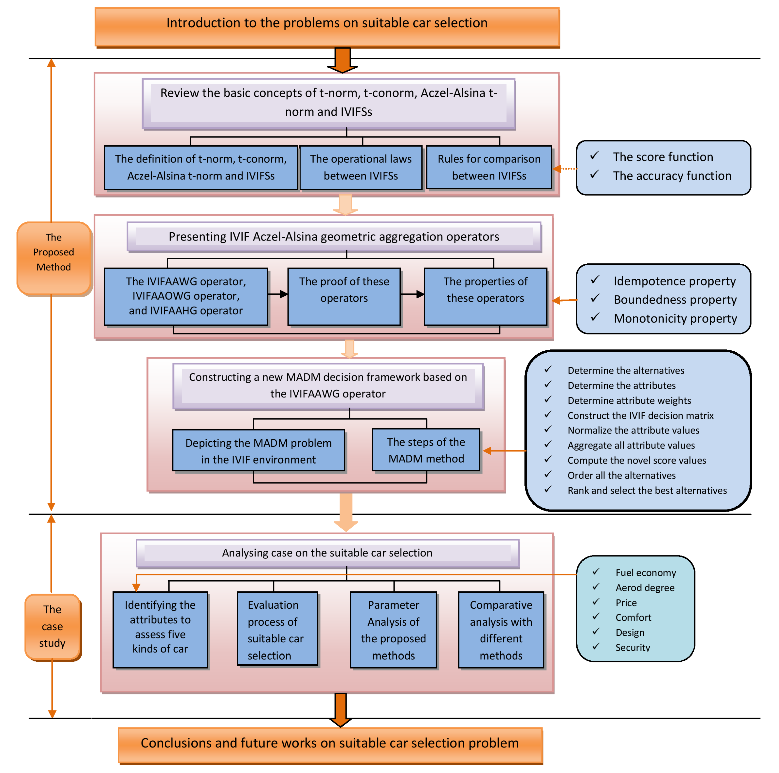
:1. Introduction
1.1. Motivation of the Study
1.2. Structure of This Study
2. Preliminaries
- (i)
- , if , , , and for all ;
- (ii)
- iff and ;
- (iii)
- for all ;
- (iv)
- (v)
- (i)
- ;
- (ii)
- ;
- (iii)
- ;
- (iv)
- ;
- (v)
- , ;
- (vi)
- , .
- (1)
- if , then ,
- (2)
- if , then
- (a)
- if , then ,
- (b)
- if , then
- (I)
- if , then ,
- (II)
- if , then
- (i)
- if , then ,
- (ii)
- if , then and are same, i.e., , , and , denoted by .
3. Aczel–Alsina Operations of IVIFNs
- (i)
- ,
- (ii)
- ,
- (i)
- ,
- (ii)
- .
- (i)
- (ii)
- (iii)
- (iv)
- .
- (i)
- ;
- (ii)
- ;
- (iii)
- , ;
- (iv)
- , ;
- (v)
- , ;
- (vi)
- , .
- (i)
- .
- (ii)
- It is simple.
- (iii)
- Let .Then, .Using this, we get .
- (iv)
- .
- (v)
- .
- (vi)
- .
4. IVIF Aczel–Alsina Geometric Aggregation Operators
5. MADM Methods Influenced by IVIFAAWG Operator
- Step 1.
- Modify decision matrix into the normalization matrix .where is the complement of , such that .
- Step 2.
- Make use of the decision data expressed in matrix , and the operator IVIFAAWG to get the overall preference values of the alternative , i.e.,
- Step 3.
- Rank all of the alternatives in order of preference. Make use of the method in Definition 3 to rank the entire rating values and rank all the alternatives as per ˜ in descending order. Lastly, we choose the advantageous alternative(s) with the highest rating value.
- Step 4.
- End.
6. Numerical Example
6.1. Problem Description
6.2. The IFAAWG Operator-Based Technique
- Step 2. Assume that . The IVIFAAWG operator is used to know the overall alternative values for five alternatives ,,,,,.
- Step 3. We evaluate the score values of the universal IVIFNs utilizing Equation (2) as , , , , .
- Step 4. Ranking these five alternatives according to the score values of the overall IVIFNs as .
- Step 5. Thus, the best car is .
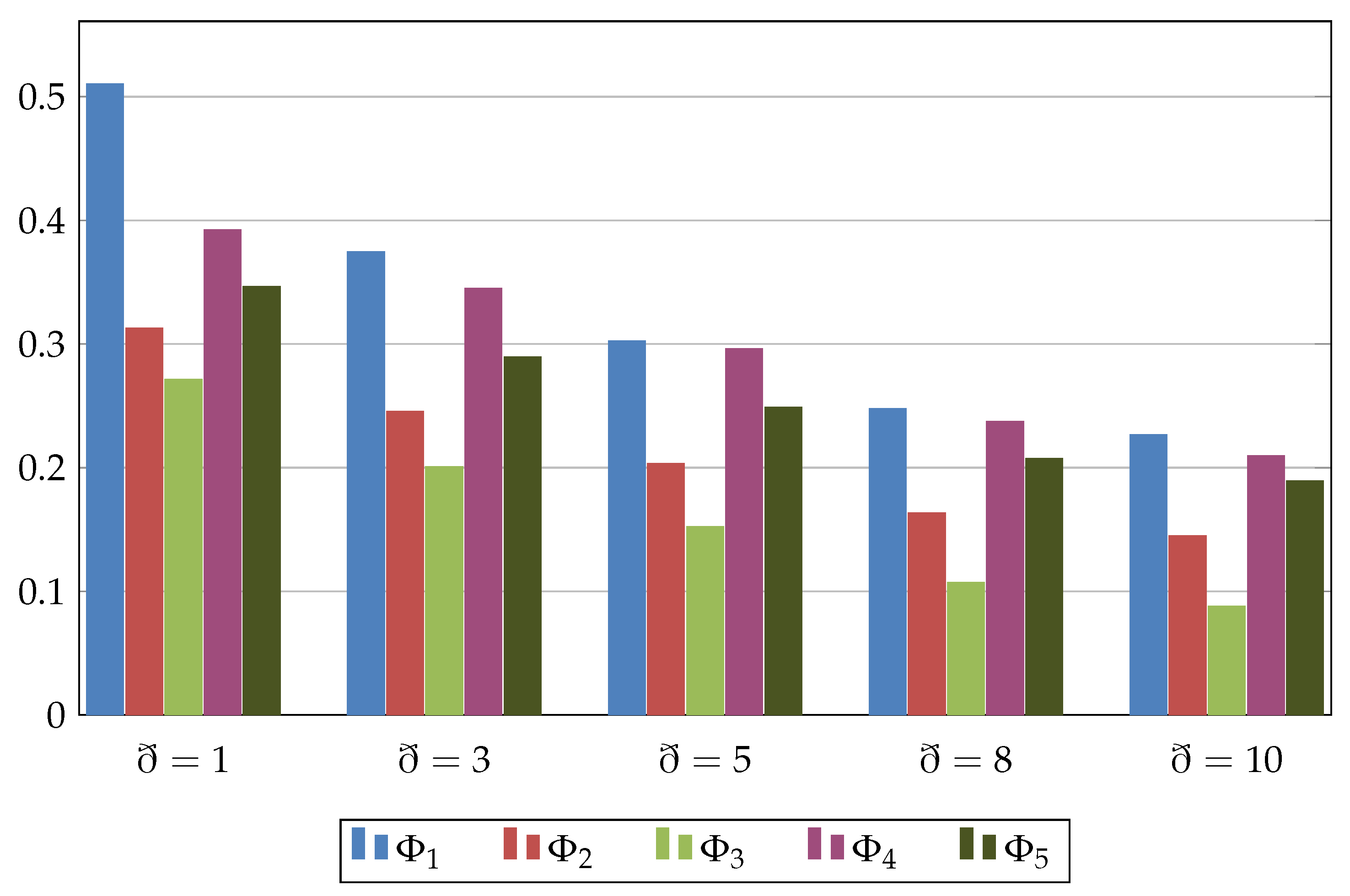
7. The Impact of the Parameter ð in This Technique
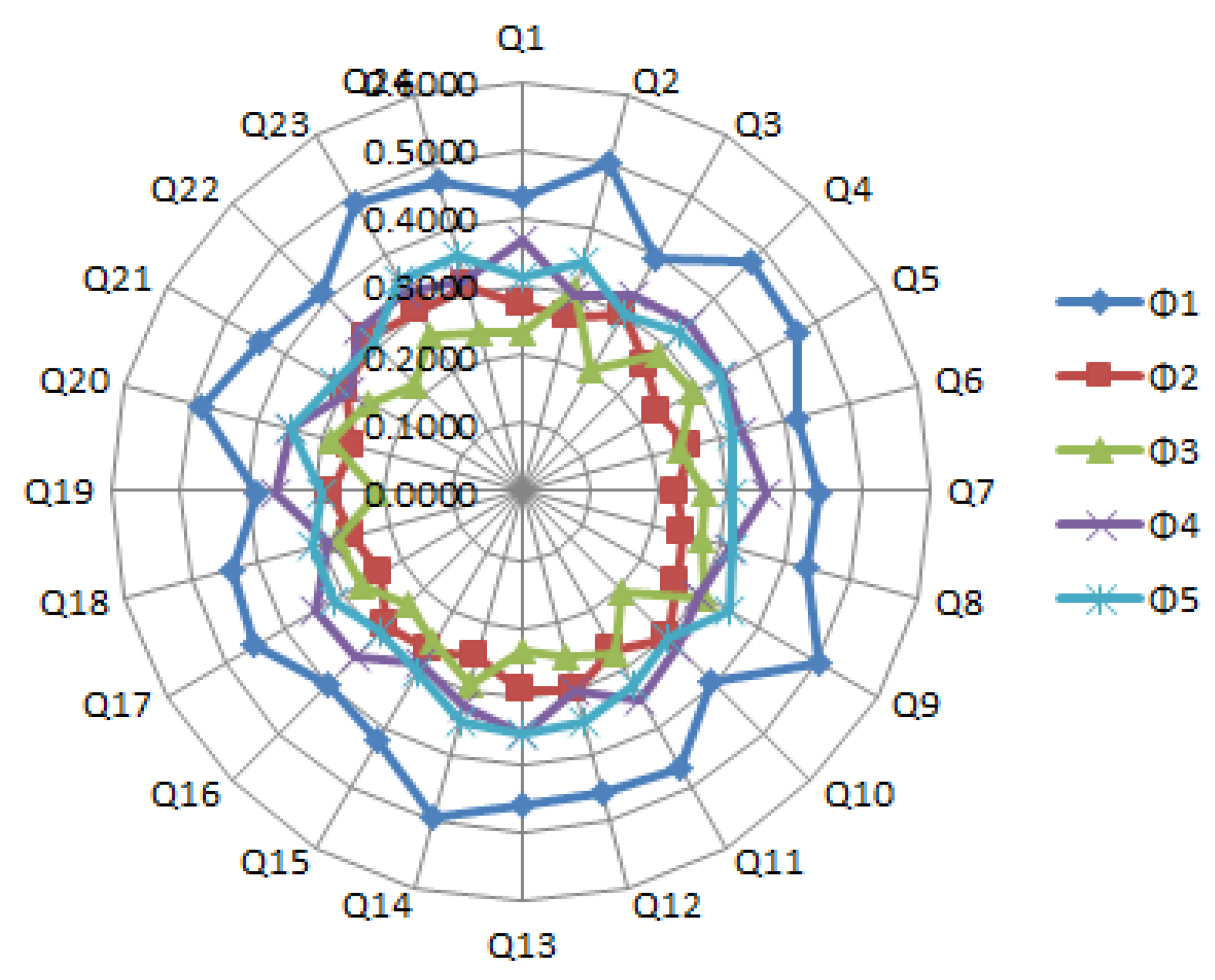
8. Sensitivity Analysis (SA) of Criteria Weights
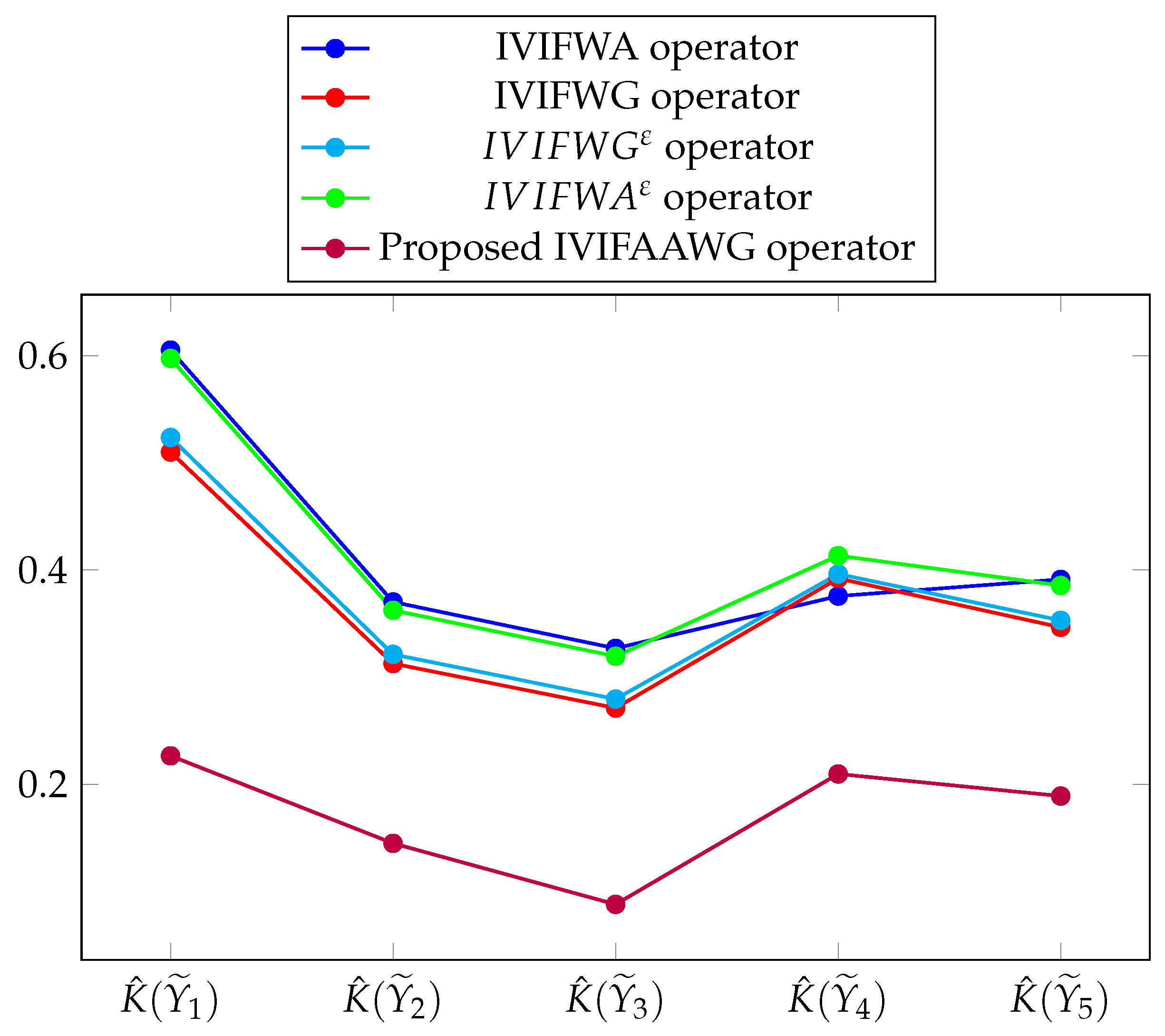
9. Comparison Study
10. Conclusions
Author Contributions
Funding
Data Availability Statement
Conflicts of Interest
Abbreviations
| IVIF | interval-valued intuitionistic fuzzy |
| IVIFS | interval-valued intuitionistic fuzzy set |
| IVIFN | interval-valued intuitionistic fuzzy number |
| MADM | multiple attribute decision making |
| IVIFWA | IVIF weighted averaging |
| IVIFHA | IVIF hybrid averaging |
| IVIF Einstein weighted averaging | |
| IVIF Einstein weighted geometric | |
| IVIFAAWG | IVIF Aczel-Alsina weighted geometric |
| IVIFAAOWG | IVIF Aczel-Alsina order weighted geometric |
| IVIFAAHG | IVIF Aczel-Alsina hybrid geometric |
References
- Attanassov, K.T. Intuitionistic fuzzy sets. Fuzzy Sets Syst. 1986, 20, 87–96. [Google Scholar] [CrossRef]
- Atanassov, K.T.; Gargov, G. Interval valued intuitionistic fuzzy sets. Fuzzy Sets Syst. 1989, 31, 343–349. [Google Scholar] [CrossRef]
- Beliakov, G.; Bustince, H.; James, S.; Calvo, T.; Fernandez, J. Aggregation for Atanassov’s intuitionistic and interval valued fuzzy sets: The median operator. IEEE Trans. Fuzzy Syst. 2012, 20, 487–498. [Google Scholar] [CrossRef]
- Chen, T.Y.; Wang, H.P.; Lu, Y.Y. A multicriteria group decision-making approach based on interval-valued intuitionistic fuzzy sets: A comparative perspective. Expert Syst. Appl. 2011, 38, 7647–7658. [Google Scholar] [CrossRef]
- Xu, Z. Methods for aggregating interval-valued intuitionistic fuzzy information and their application to decision making. Control Decis. 2007, 22, 215–219. [Google Scholar]
- Liu, P. Multiple attribute group decision making method based on interval-valued intuitionistic fuzzy power Heronian aggregation operators. Comput. Ind. Eng. 2017, 108, 199–212. [Google Scholar] [CrossRef]
- Zhao, H.; Xu, Z. Group decision making with density-based aggregation operators under interval-valued intuitionistic fuzzy environments. J. Intell. Fuzzy Syst. 2014, 27, 1021–1033. [Google Scholar] [CrossRef]
- Yu, D.; Wu, Y.; Lu, T. Interval-valued intuitionistic fuzzy prioritized operators and their application in group decision making. Know-Based Syst. 2012, 30, 57–66. [Google Scholar] [CrossRef]
- Chen, S.M.; Han, W.H. A new multiattribute decision making method based on multiplication operations of interval-valued intuitionistic fuzzy values and linear programming methodology. Inf. Sci. 2018, 429, 421–432. [Google Scholar] [CrossRef]
- Chen, S.M.; Han, W.H. Multiattribute decision making based on nonlinear programming methodology, particle swarm optimization techniques and interval-valued intuitionistic fuzzy values. Inf. Sci. 2019, 471, 252–268. [Google Scholar] [CrossRef]
- Wei, G.; Wang, X. Some geometric aggregation operators based on interval-valued intuitionistic fuzzy sets and their application to group decision making. In Proceedings of the 2007 International Conference on Computational Intelligence and Security (CIS 2007), Harbin, China, 15–19 December 2007; pp. 495–499. [Google Scholar]
- Li, D.F. TOPSIS-based nonlinear-programming methodology for multiattribute decision making with interval-valued intuitionistic fuzzy sets. IEEE Trans. Fuzzy Syst. 2010, 18, 299–311. [Google Scholar] [CrossRef]
- Xu, Z.; Gou, X. An overview of interval-valued intuitionistic fuzzy information aggregations and applications. Granul. Comput. 2017, 2, 13–39. [Google Scholar] [CrossRef]
- Chen, S.M.; Kuo, L.W.; Zou, X.Y. Multiattribute decision making based on Shannon’s information entropy, non-linear programming methodology, and interval-valued intuitionistic fuzzy values. Inf. Sci. 2018, 465, 404–424. [Google Scholar] [CrossRef]
- Meng, F.Y.; Cheng, H.; Zhang, Q. Induced Atanassov’s inter-valvalued intuitionistic fuzzy hybrid Choquet integral operators and their application in decision making. Int. J. Comput. Intell. Syst. 2014, 7, 524–542. [Google Scholar] [CrossRef] [Green Version]
- Wang, W.; Liu, X. The multi-attribute decision making method based on interval-valued intuitionistic fuzzy Einstein hybrid weighted geometric operator. Comput. Math. Appl. 2013, 66, 1845–1856. [Google Scholar] [CrossRef]
- Wang, W.; Liu, X. Interval-valued intuitionistic fuzzy hybrid weighted averaging operator based on Einstein operation and its application to decision making. J. Intell. Fuzzy Syst. 2013, 25, 279–290. [Google Scholar] [CrossRef]
- Cheng, S.H. Autocratic multiattribute group decision making for hotel location selection based on interval-valued intuitionistic fuzzy sets. Inf. Sci. 2018, 427, 77–87. [Google Scholar] [CrossRef]
- Chen, S.M.; Cheng, S.H.; Tsai, W.H. Multiple attribute group decision making based on interval-valued intuitionistic fuzzy aggregation operators and transformation techniques of interval-valued intuitionistic fuzzy values. Inf. Sci. 2016, 367–368, 418–442. [Google Scholar] [CrossRef]
- Abdullah, L.; Zulkifli, N.; Liao, H.; Herrera-Viedma, E.; Al-Barakati, A. An interval-valued intuitionistic fuzzy DEMATEL method combined with Choquet integral for sustainable solid waste management. Eng. Appl. Artif. Intel. 2019, 82, 207–215. [Google Scholar] [CrossRef]
- Liu, H.C.; Quan, M.Y.; Li, Z.W.; Wang, Z.L. A new integrated MCDM model for sustainable supplier selection under interval-valued intuitionistic uncertain linguistic environment. Inf. Sci. 2019, 486, 254–270. [Google Scholar] [CrossRef]
- Meng, F.; Tang, J.; Wang, P.; Chen, X. A programming-based algorithm for interval-valued intuitionistic fuzzy group decision making. Knowl. Based Syst. 2018, 144, 122–143. [Google Scholar] [CrossRef]
- Kong, D.; Chang, T.; Pan, J.; Hao, N.; Yang, G. A decision variable-based combinatorial optimization approach for interval-valued intuitionistic fuzzy MAGDM. Inf. Sci. 2019, 484, 197–218. [Google Scholar] [CrossRef]
- Schweizer, B.; Sklar, A. Statistical metric spaces. Pacific J. Math. 1960, 10, 313–334. [Google Scholar] [CrossRef] [Green Version]
- Deschrijver, G.; Cornelis, C.; Kerre, E.E. On the representation of intuitionistic fuzzy t-norms and t-conorms. IEEE Trans. Fuzzy Syst. 2004, 12, 45–61. [Google Scholar] [CrossRef]
- Liu, P. Some Hamacher aggregation operators based on the interval-valued intuitionistic fuzzy numbers and their application to group decision making. IEEE Trans. Fuzzy Syst. 2014, 22, 83–97. [Google Scholar] [CrossRef]
- Yu, D. Group decision making under interval-valued multiplicative intuitionistic fuzzy environment based on Archimedean t-conorm and t-norm. Int. J. Intell. Syst. 2015, 30, 590–616. [Google Scholar] [CrossRef]
- Klement, E.P.; Mesiar, R.; Pap, E. Triangular Norms; Kluwer Academic Publishers: Dordrecht, The Netherlands, 2000. [Google Scholar]
- Menger, K. Statistical metrics. Proc. Natl. Acad. Sci. USA 1942, 8, 535–537. [Google Scholar] [CrossRef] [Green Version]
- Zadeh, L.A. Fuzzy sets. Inform. Control 1965, 8, 338–353. [Google Scholar] [CrossRef] [Green Version]
- Schweizer, B.; Sklar, A. Associative functions and statistical triangle inequalities. Publ. Math. Debrecen 1961, 8, 169–186. [Google Scholar]
- Goguen, J.A. L-fuzzy sets. J. Math. Anal. Appl. 1967, 8, 145–174. [Google Scholar] [CrossRef] [Green Version]
- Aczel, J.; Alsina, C. Characterization of some classes of quasilinear functions with applications to triangular norms and to synthesizing judgements. Aequationes Math. 1982, 25, 313–315. [Google Scholar] [CrossRef]
- Wang, N.; Li, Q.; El-Latif, A.A.A.; Yan, X.; Niu, X. A Novel Hybrid Multibiometrics Based on the Fusion of Dual Iris, Visible and Thermal Face Images. In Proceedings of the 2013 International Symposium on Biometrics and Security Technologies, Chengdu, China, 2–5 July 2013; pp. 217–223. [Google Scholar] [CrossRef]
- Senapati, T.; Chen, G.; Yager, R.R. Aczel-Alsina aggregation operators and their application to intuitionistic fuzzy multiple attribute decision making. Int. J. Intell. Syst. 2022, 37, 1529–1551. [Google Scholar] [CrossRef]
- Senapati, T.; Chen, G.; Mesiar, R.; Yager, R.R. Novel Aczel–Alsina operations-based interval-valued intuitionistic fuzzy aggregation operatorsandtheir applications in multiple attribute decision-making process. Int. J. Intell. Syst. 2021, 1–23. [Google Scholar] [CrossRef]
- Senapati, T.; Chen, G.; Mesiar, R.; Yager, R.R.; Saha, A. Novel Aczel-Alsina operations-based hesitant fuzzy aggregation operators and their applications in cyclone disaster assessment. Int. J. Gen. Syst. 2022, 1–39. [Google Scholar] [CrossRef]
- Senapati, T. Approaches to multi-attribute decision-making based on picture fuzzy Aczel–Alsina average aggregation operators. Comp. Appl. Math. 2022, 41, 40. [Google Scholar] [CrossRef]
- Xu, Z.; Chen, J. On geometric aggregation over interval-valued intuitionistic fuzzy information. In Proceedings of the Fourth International Conference on Fuzzy Systems and Knowledge Discovery (FSKD 07), Haikou, China, 24–27 August 2007; Volume 2, pp. 466–471. [Google Scholar]
- Wang, Z.; Li, K.W.; Wang, W. An approach to multiattribute decision making with interval-valued intuitionistic fuzzy assessments and incomplete weights. Inf. Sci. 2009, 179, 3026–3040. [Google Scholar] [CrossRef] [Green Version]
- Deschrijver, G.; Kerre, E. On the relationship between some extensions of fuzzy set theory. Fuzzy Sets Syst. 2003, 133, 227–235. [Google Scholar] [CrossRef]
- Miguel, D.L.; Bustince, H.; Fernandez, J.; Indurain, E.; Kolesarova, A.; Mesiar, R. Construction of admissible linear orders for interval-valued Atanassov intuitionistic fuzzy sets with an application to decisionmaking. Inf. Fusion 2016, 27, 189–197. [Google Scholar] [CrossRef]
- De Miguel, L.; Bustince, H.; Pekala, B.; Bentkowska, U.; Da Silva, I.; Bedregal, B.; Mesiar, R.; Ochoa, G. Interval-valued Atanassov intuitionistic OWA aggregations using admissible linear orders and their application to decision making. IEEE Trans. Fuzzy Syst. 2016, 24, 1586–1597. [Google Scholar] [CrossRef] [Green Version]
- Herrera, E.; Martinez, L. An approach for combining linguistic and numerical information based on 2-tuple fuzzy linguistic representation model in decision-making. Int. J. Uncertain. Fuzziness Knowl. Based Syst. 2000, 8, 539–562. [Google Scholar] [CrossRef]
- Beg, I.; Rashid, T. Group decision making using intuitionistic hesitant fuzzy sets. Int. J. Fuzzy Log. Intell. 2014, 14, 181–187. [Google Scholar] [CrossRef] [Green Version]
- Saha, A.; Simic, V.; Senapati, T.; Dabic-Miletic, S.; Ala, A. A dual hesitant fuzzy sets-based methodology for advantage prioritization of zero-emission last-mile delivery solutions for sustainable city logistics. IEEE Trans. Fuzzy Syst. 2022. [Google Scholar] [CrossRef]
- Tan, J.; Liu, Y.; Senapati, T.; Garg, H.; Rong, Y. An extended MABAC method based on prospect theory with unknown weight information under Fermatean fuzzy environment for risk investment assessment in B&R. J. Ambient. Intell. Humaniz. Comput. 2022. [Google Scholar] [CrossRef]
- Sahoo, L.; Sen, S.; Tiwary, K.; Samanta, S.; Senapati, T. Modified Floyd-Warshall’s algorithm for maximum connectivity in Wireless Sensor Networks under uncertainty. Discrete Dyn. Nat. Soc. 2022, 2022, 5973433. [Google Scholar] [CrossRef]
- Sergi, D.; Sari, I.U.; Senapati, T. Extension of capital budgeting techniques using interval-valued Fermatean fuzzy sets. J. Intell. Fuzzy Syst. 2022, 42, 365–376. [Google Scholar] [CrossRef]
- Ibrar, M.; Khan, A.; Khan, S.; Abbas, F. Fuzzy parameterized bipolar fuzzy soft expert set and its application in decision making. Int. J. Fuzzy Log. Intell. 2019, 19, 234–241. [Google Scholar] [CrossRef] [Green Version]
- Saha, A.; Senapati, T.; Yager, R.R. Hybridizations of generalized Dombi operators and Bonferroni mean operators under dual probabilistic linguistic environment for group decision-making. Int. J. Intell. Syst. 2021, 36, 6645–6679. [Google Scholar] [CrossRef]
- Senapati, T.; Yager, R.R. Fermatean fuzzy weighted averaging/geometric operators and its application in multi-criteria decision-making methods. Eng. Appl. Artif. Intel. 2019, 85, 112–121. [Google Scholar] [CrossRef]
- Senapati, T.; Yager, R.R. Some new operations over Fermatean fuzzy numbers and application of Fermatean fuzzy WPM in multiple criteria decision making. Informatica 2019, 30, 391–412. [Google Scholar] [CrossRef] [Green Version]
- Senapati, T.; Yager, R.R. Fermatean fuzzy sets. J. Ambient. Intell. Humaniz. Comput. 2020, 11, 663–674. [Google Scholar] [CrossRef]
- Mesiar, R.; Kolesarova, A.; Senapati, T. Aggregation on lattices isomorphic to the lattice of closed subintervals of the real unit interval. Fuzzy Sets Syst. 2022. [Google Scholar] [CrossRef]
- Senapati, T.; Chen, G. Picture fuzzy WASPAS technique and its application in multi-criteria decision-making. Soft Comput. 2022. [Google Scholar] [CrossRef]
- Senapati, T.; Chen, G. Some novel interval-valued Pythagorean fuzzy aggregation operator based on Hamacher triangular norms and their application in MADM issues. Comp. Appl. Math. 2021, 40, 109. [Google Scholar] [CrossRef]
- Senapati, T.; Yager, R.R.; Chen, G. Cubic intuitionistic WASPAS technique and its application in multi-criteria decision-making. J. Ambient. Intell. Humaniz. Comput. 2021, 12, 8823–8833. [Google Scholar] [CrossRef]


| ([0.56,0.66],[0.26,0.31]) | ([0.38,0.47],[0.34,0.44]) | ([0.56,0.63],[0.23,0.32]) | ([0.64,0.73],[0.16,0.27]) | ([0.48,0.63],[0.26,0.36]) | |
| ([0.78,0.88],[0.07,0.12]) | ([0.47,0.56],[0.27,0.37]) | ([0.51,0.57],[0.16,0.26]) | ([0.65,0.75],[0.13,0.20]) | ([0.64,0.69],[0.21,0.31]) | |
| ([0.61,0.82],[0.11,0.18]) | ([0.79,0.84],[0.11,0.16]) | ([0.51,0.56],[0.36,0.44]) | ([0.54,0.64],[0.25,0.36]) | ([0.79,0.84],[0.08,0.16]) | |
| ([0.82,0.91],[0.02,0.07]) | ([0.55,0.65],[0.22,0.32]) | ([0.63,0.74],[0.21,0.25]) | ([0.65,0.75],[0.20,0.25]) | ([0.60,0.73],[0.17,0.27]) | |
| ([0.44,0.56],[0.32,0.42]) | ([0.68,0.78],[0.17,0.22]) | ([0.35,0.45],[0.35,0.45]) | ([0.59,0.69],[0.25,0.30]) | ([0.45,0.54],[0.35,0.45]) | |
| ([0.70,0.83],[0.08,0.17]) | ([0.53,0.58],[0.31,0.36]) | ([0.76,0.83],[0.07,0.17]) | ([0.41,0.51],[0.36,0.42]) | ([0.56,0.66],[0.22,0.32]) |
| ð | Ranking Order | |||||
|---|---|---|---|---|---|---|
| 1 | 0.510021 | 0.312610 | 0.271095 | 0.392077 | 0.346408 | |
| 2 | 0.432522 | 0.274768 | 0.232654 | 0.369262 | 0.315391 | |
| 3 | 0.374209 | 0.245251 | 0.200569 | 0.344796 | 0.289366 | |
| 4 | 0.332473 | 0.222023 | 0.174023 | 0.319924 | 0.267292 | |
| 5 | 0.302133 | 0.203274 | 0.152149 | 0.295960 | 0.248489 | |
| 6 | 0.279331 | 0.187738 | 0.134129 | 0.273905 | 0.232478 | |
| 7 | 0.261630 | 0.174584 | 0.119238 | 0.254265 | 0.218860 | |
| 8 | 0.247512 | 0.163268 | 0.106868 | 0.237122 | 0.207273 | |
| 9 | 0.236003 | 0.153420 | 0.096520 | 0.222303 | 0.197390 | |
| 10 | 0.226454 | 0.144778 | 0.087797 | 0.209530 | 0.188927 |
| Weight Sets | Weight Sets | ||||||||||||
|---|---|---|---|---|---|---|---|---|---|---|---|---|---|
| Q1 | 0.15 | 0.25 | 0.14 | 0.16 | 0.20 | 0.10 | Q13 | 0.16 | 0.20 | 0.25 | 0.15 | 0.14 | 0.10 |
| Q2 | 0.15 | 0.14 | 0.16 | 0.20 | 0.10 | 0.25 | Q14 | 0.16 | 0.25 | 0.15 | 0.14 | 0.10 | 0.20 |
| Q3 | 0.15 | 0.16 | 0.20 | 0.10 | 0.25 | 0.14 | Q15 | 0.16 | 0.15 | 0.14 | 0.10 | 0.20 | 0.25 |
| Q4 | 0.15 | 0.20 | 0.10 | 0.25 | 0.14 | 0.16 | Q16 | 0.16 | 0.14 | 0.10 | 0.20 | 0.25 | 0.15 |
| Q5 | 0.25 | 0.15 | 0.14 | 0.20 | 0.10 | 0.16 | Q17 | 0.20 | 0.25 | 0.10 | 0.14 | 0.15 | 0.16 |
| Q6 | 0.25 | 0.14 | 0.20 | 0.10 | 0.16 | 0.15 | Q18 | 0.20 | 0.10 | 0.14 | 0.15 | 0.16 | 0.25 |
| Q7 | 0.25 | 0.20 | 0.10 | 0.16 | 0.15 | 0.14 | Q19 | 0.20 | 0.14 | 0.15 | 0.16 | 0.25 | 0.10 |
| Q8 | 0.25 | 0.10 | 0.16 | 0.15 | 0.14 | 0.20 | Q20 | 0.20 | 0.15 | 0.16 | 0.25 | 0.10 | 0.14 |
| Q9 | 0.14 | 0.16 | 0.15 | 0.20 | 0.10 | 0.25 | Q21 | 0.10 | 0.14 | 0.15 | 0.16 | 0.20 | 0.25 |
| Q10 | 0.14 | 0.15 | 0.20 | 0.10 | 0.25 | 0.16 | Q22 | 0.10 | 0.15 | 0.16 | 0.20 | 0.25 | 0.14 |
| Q11 | 0.14 | 0.20 | 0.10 | 0.25 | 0.16 | 0.15 | Q23 | 0.10 | 0.16 | 0.20 | 0.25 | 0.14 | 0.15 |
| Q12 | 0.14 | 0.10 | 0.25 | 0.16 | 0.15 | 0.20 | Q24 | 0.10 | 0.20 | 0.25 | 0.14 | 0.15 | 0.16 |
| Ranking Order | Ranking Order | Ranking Order | |||
|---|---|---|---|---|---|
| Q1 | Q9 | Q17 | |||
| Q2 | Q10 | Q18 | |||
| Q3 | Q11 | Q19 | |||
| Q4 | Q12 | Q20 | |||
| Q5 | Q13 | Q21 | |||
| Q6 | Q14 | Q22 | |||
| Q7 | Q15 | Q23 | |||
| Q8 | Q16 | Q24 |
| Techniques | Preference Order | |||||
|---|---|---|---|---|---|---|
| Xu [5] | 0.605185 | 0.370086 | 0.326785 | 0.375578 | 0.391143 | |
| Xu & Chen [39] | 0.510021 | 0.312610 | 0.271095 | 0.392077 | 0.346408 | |
| Wang & Liu [16] | 0.523568 | 0.321157 | 0.279447 | 0.396147 | 0.352904 | |
| Wang & Liu [17] | 0.597400 | 0.362337 | 0.319370 | 0.413345 | 0.385472 | |
| Proposed method | 0.226454 | 0.144778 | 0.087797 | 0.209530 | 0.188927 |
Publisher’s Note: MDPI stays neutral with regard to jurisdictional claims in published maps and institutional affiliations. |
© 2022 by the authors. Licensee MDPI, Basel, Switzerland. This article is an open access article distributed under the terms and conditions of the Creative Commons Attribution (CC BY) license (https://creativecommons.org/licenses/by/4.0/).
Share and Cite
Senapati, T.; Mesiar, R.; Simic, V.; Iampan, A.; Chinram, R.; Ali, R. Analysis of Interval-Valued Intuitionistic Fuzzy Aczel–Alsina Geometric Aggregation Operators and Their Application to Multiple Attribute Decision-Making. Axioms 2022, 11, 258. https://doi.org/10.3390/axioms11060258
Senapati T, Mesiar R, Simic V, Iampan A, Chinram R, Ali R. Analysis of Interval-Valued Intuitionistic Fuzzy Aczel–Alsina Geometric Aggregation Operators and Their Application to Multiple Attribute Decision-Making. Axioms. 2022; 11(6):258. https://doi.org/10.3390/axioms11060258
Chicago/Turabian StyleSenapati, Tapan, Radko Mesiar, Vladimir Simic, Aiyared Iampan, Ronnason Chinram, and Rifaqat Ali. 2022. "Analysis of Interval-Valued Intuitionistic Fuzzy Aczel–Alsina Geometric Aggregation Operators and Their Application to Multiple Attribute Decision-Making" Axioms 11, no. 6: 258. https://doi.org/10.3390/axioms11060258