
Investigation into the Explicit Solutions of the Integrable (2+1)—Dimensional Maccari System via the Variational Approach


Abstract
:1. Introduction
2. The VP
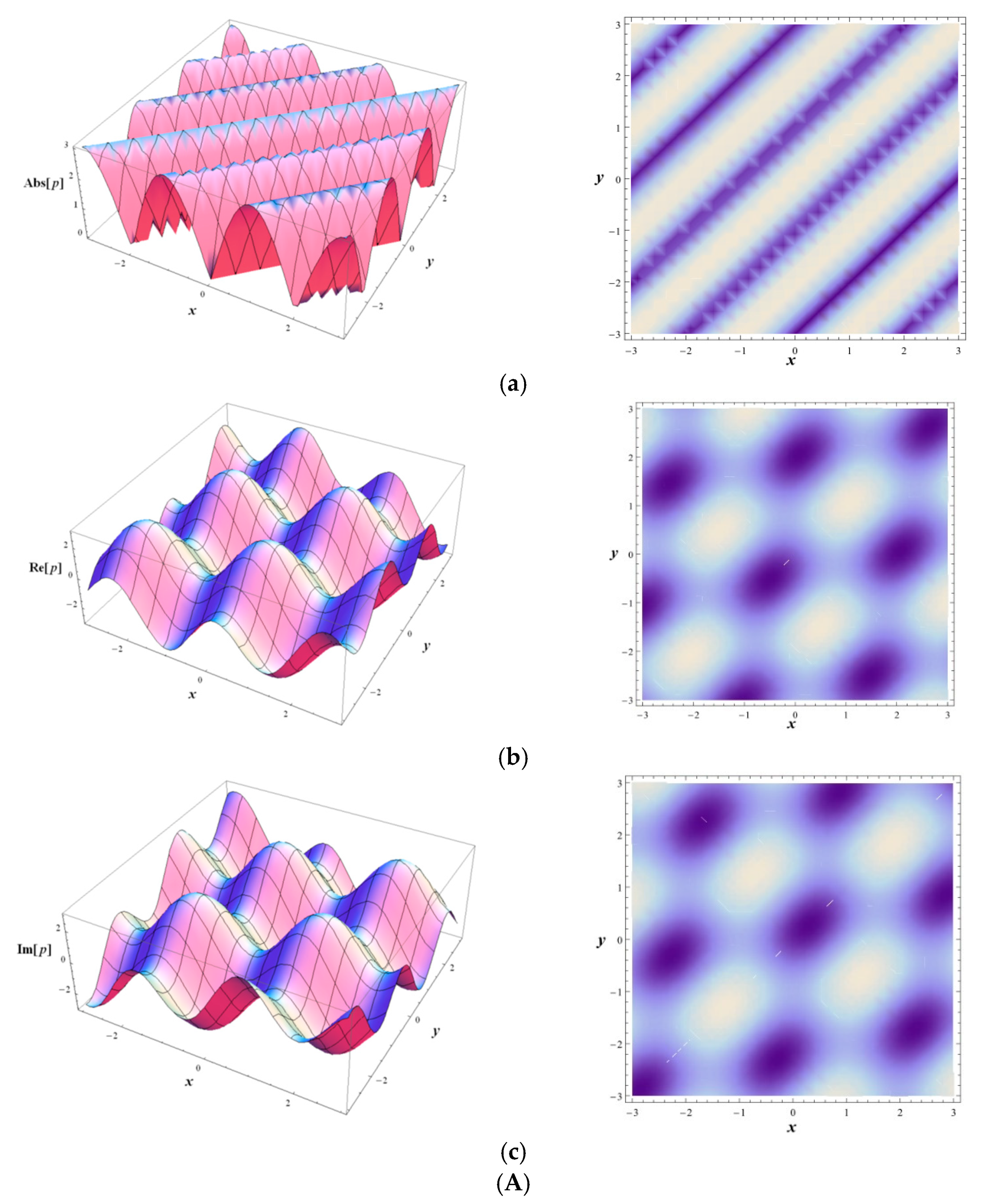
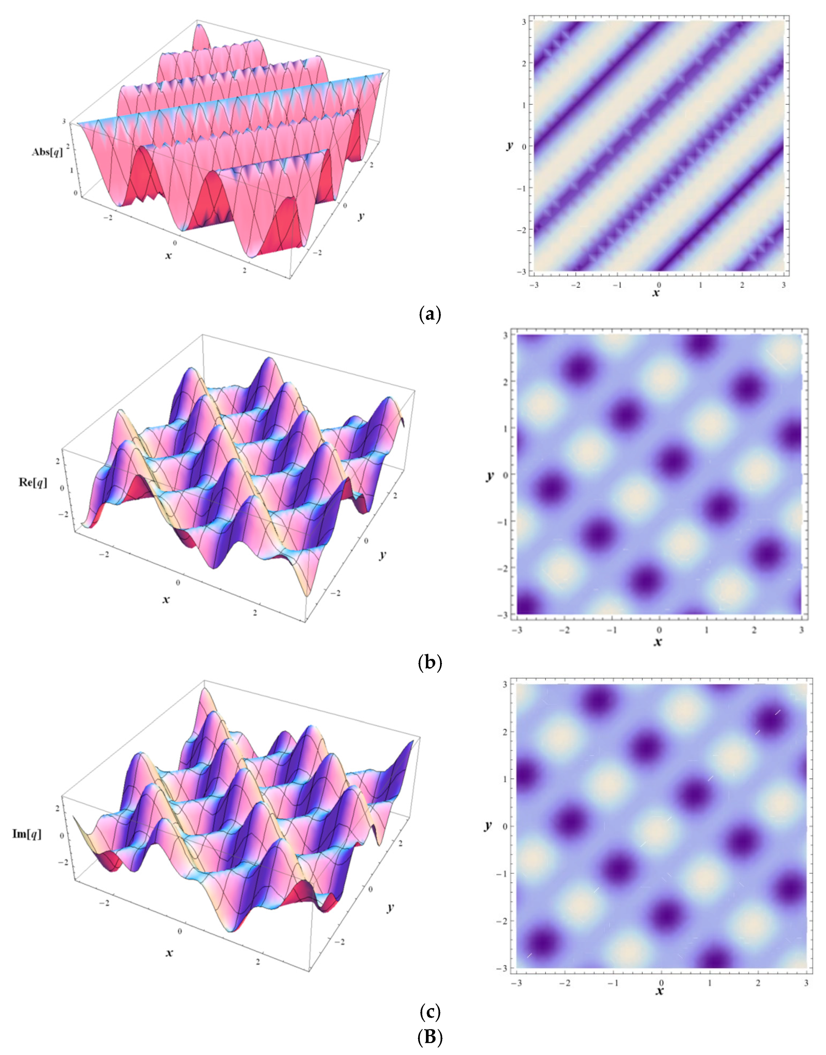
3. The PWSs
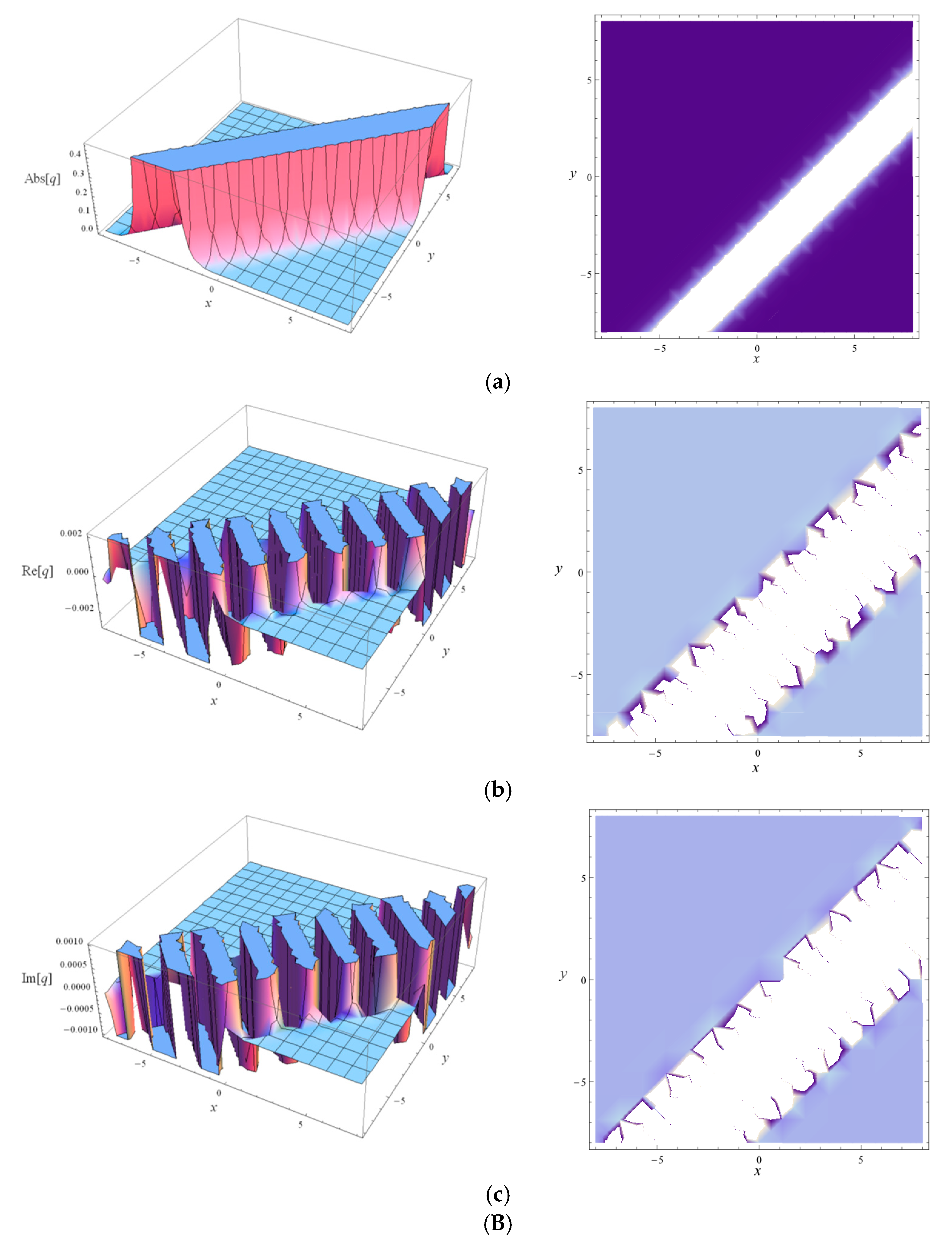
4. The SWSs
5. Numerical Results and Discussion
6. Conclusions and Future Research
Author Contributions
Funding
Institutional Review Board Statement
Data Availability Statement
Acknowledgments
Conflicts of Interest
References
- Ding, B.; Zhang, Z.H.; Gong, L.; Xu, M.-H.; Huang, Z.-Q. A novel thermal management scheme for 3D-IC chips with multi-cores and high power density. Appl. Therm. Eng. 2020, 168, 114832. [Google Scholar] [CrossRef]
- Sivakumar, P.; Pandiaraj, K.; JeyaPrakash, K. Optimization of thermal aware multilevel routing for 3D IC. Analog. Integr. Circuits Signal Processing 2020, 103, 131–142. [Google Scholar] [CrossRef]
- Elshaari, A.W.; Pernice, W.; Srinivasan, K.; Benson, O.; Zwiller, V. Hybrid integrated quantum photonic circuits. Nat. Photonics 2020, 14, 285–298. [Google Scholar] [CrossRef] [PubMed]
- Khater, M.M.A.; Attia, R.A.M.; Alodhaibi, S.S.; Lu, D. Novel soliton waves of two fluid nonlinear evolutions models in the view of computational scheme. Int. J. Mod. Phys. B. 2020, 34, 2050096. [Google Scholar] [CrossRef]
- Imran, N.; Javed, M.; Sohail, M.; Thounthong, P.; Abdelmalek, Z. Theoretical exploration of thermal transportation with chemical reactions for sutterby fluid model obeying peristaltic mechanism. J. Mater. Res. Technol. 2020, 9, 7449–7459. [Google Scholar]
- Sohai, M.; Nazir, l.; Bazighifan, O.; El-Nabulsi, R.A.; Selim, M.M.; Alrabaiah, H.; Thounthong, P. Significant involvement of double diffusion theories on viscoelastic fluid comprising variable thermophysical properties. Micromachines 2021, 12, 951. [Google Scholar] [CrossRef]
- Wang, K.J. Traveling wave solutions of the Gardner equation in dusty plasmas. Results Phys. 2022, 33, 105207. [Google Scholar]
- Saha Ray, S.; Sagar, B. Numerical Soliton Solutions of Fractional Modified (2+1)-Dimensional Konopelchenko–Dubrovsky Equations in Plasma Physics. J. Comput. Nonlinear Dyn. 2022, 17, 011007. [Google Scholar] [CrossRef]
- Ali, K.K.; Yilmazer, R.; Baskonus, H.M.; Bulut, H. New wave behaviors and stability analysis of the Gilson–Pickering equation in plasma physics. Indian J. Phys. 2021, 95, 1003–1008. [Google Scholar] [CrossRef]
- Ali, K.K.; Wazwaz, A.M.; Osman, M.S. Optical soliton solutions to the generalized nonautonomous nonlinear Schrödinger equations in optical fibers via the sine-Gordon expansion method. Optik 2020, 208, 164132. [Google Scholar]
- Attia, R.A.M.; Lu, D.; Ak, T.; Khater, M.M.A. Optical wave solutions of the higher-order nonlinear Schrödinger equation with the non-Kerr nonlinear term via modified Khater method. Mod. Phys. Lett. B 2020, 34, 2050044. [Google Scholar] [CrossRef]
- Wang, K.J. Periodic solution of the time-space fractional complex nonlinear Fokas-Lenells equation by an ancient Chinese algorithm. Optik 2021, 243, 167461. [Google Scholar] [CrossRef]
- Biswas, A. Optical soliton cooling with polynomial law of nonlinear refractive index. J. Opt. 2020, 49, 580–583. [Google Scholar] [CrossRef]
- Wang, L.; Luan, Z.; Zhou, Q.; Biswas, A.; Alzahrani, A.K.; Liu, W. Effects of dispersion terms on optical soliton propagation in a lossy fiber system. Nonlinear Dyn. 2021, 104, 629–637. [Google Scholar] [CrossRef]
- Wang, K.J. Abundant exact soliton solutions to the Fokas system. Optik 2022, 249, 168265. [Google Scholar] [CrossRef]
- Attia, R.A.M.; Baleanu, D.; Lu, D.; Khater, M.M.A.; Ahmed, E.-S. Computational and numerical simulations for the deoxyribonucleic acid (DNA) model. Discret. Contin. Dyn. Syst. S 2021, 14, 3459. [Google Scholar] [CrossRef]
- Baleanu, D.; Mohammadi, H.; Rezapour, S. Analysis of the model of HIV-1 infection of CD4+ T-cell with a new approach of fractional derivative. Adv. Differ. Equ. 2020, 2020, 71. [Google Scholar] [CrossRef] [Green Version]
- Khater, M.M.A.; Attia, R.A.M.; Abdel-Aty, A.H.; Alharbi, W.; Lu, D. Abundant analytical and numerical solutions of the fractional microbiological densities model in bacteria cell as a result of diffusion mechanisms. Chaos Solitons Fractals 2020, 136, 109824. [Google Scholar] [CrossRef]
- Ren, X.; Tian, Y.; Liu, L.; Liu, X. A reaction–diffusion within-host HIV model with cell-to-cell transmission. J. Math. Biol. 2018, 76, 1831–1872. [Google Scholar] [CrossRef]
- He, J.H.; Yang, Q.; He, C.H.; Khan, Y. A simple frequency formulation for the tangent oscillator. Axioms 2021, 10, 320. [Google Scholar] [CrossRef]
- Salas, A.H.; El-Tantawy, S.A.; Aljahdaly, N.H. An exact solution to the quadratic damping strong nonlinearity Duffing oscillator. Math. Probl. Eng. 2021, 2021, 8875589. [Google Scholar] [CrossRef]
- Wang, K.J. Research on the nonlinear vibration of carbon nanotube embedded in fractal medium. Fractals 2022, 30, 2250016. [Google Scholar] [CrossRef]
- Ren, Z.Y. A simplified He’s frequency–amplitude formulation for nonlinear oscillators. J. Low Freq. Noise Vib. Act. Control. 2022, 41, 14613484211030737. [Google Scholar] [CrossRef]
- Anjum, N.; Ul Rahman, J.; He, J.H.; Alam, M.N.; Suleman, M. An Efficient Analytical Approach for the Periodicity of Nano/Microelectromechanical Systems’ Oscillators. Math. Probl. Eng. 2022, 2022, 9712199. [Google Scholar] [CrossRef]
- Janani, M.; Devadharshini, S.; Hariharan, G. Analytical expressions of amperometric enzyme kinetics pertaining to the substrate concentration using wavelets. J. Math. Chem. 2019, 57, 1191–1200. [Google Scholar] [CrossRef]
- Loghambal, S.; Rajendran, L. Mathematical modeling in amperometric oxidase enzyme-membrane electrodes. J. Membr. Sci. 2011, 373, 20–28. [Google Scholar] [CrossRef]
- Cheemaa, N.; Younis, M. New and more exact traveling wave solutions to integrable (2+1)-dimensional Maccari system. Nonlinear Dyn. 2016, 83, 1395–1401. [Google Scholar] [CrossRef]
- Raza, N.; Jhangeer, A.; Rezazadeh, H.; Bekir, A. Explicit solutions of the (2+ 1)-dimensional Hirota-Maccari system arising in nonlinear optics. Int. J. Mod. Phys. B 2019, 33, 1950360. [Google Scholar] [CrossRef]
- He, J.-H. A family of variational principles for compressible rotational blade-toblade flow using semi-inverse method. Int. J. Turbo Jet Engines 1998, 15, 95–100. [Google Scholar]
- He, J.-H. Semi-Inverse method of establishing generalized variational principles for fluid mechanics with emphasis on turbomachinery aerodynamics. Int. J. Turbo Jet Engines 1997, 14, 23–28. [Google Scholar] [CrossRef]
- Wang, K.J.; Wang, G.D. Solitary waves of the fractal regularized long wave equation travelling along an unsmooth boundary. Fractals 2022, 30, 2250008. [Google Scholar] [CrossRef]
- Cao, X.Q.; Hou, S.C.; Guo, Y.N.; Zhang, C.H. Variational principle for (2+1)-dimensional Broer–Kaup equations with fractal derivatives. Fractals 2020, 28, 2050107. [Google Scholar] [CrossRef]
- He, J.H. Variational principle for the generalized KdV-burgers equation with fractal derivatives for shallow water waves. J. Appl. Comput. Mech. 2020, 6, 735–740. [Google Scholar]
- He, J.H.; Sun, C. A variational principle for a thin film equation. J. Math. Chem. 2019, 57, 2075–2081. [Google Scholar] [CrossRef]
- He, J.H. Variational principle and periodic solution of the Kundu-Mukherjee-Naskar equation. Results Phys. 2020, 17, 103031. [Google Scholar] [CrossRef]
- Wang, K.J.; Shi, F.; Liu, J.H. A fractal modification of the Sharma-Tasso-Olver equation and its fractal generalized variational principle. Fractals 2022. [Google Scholar] [CrossRef]
- He, J.H. Lagrange crisis and generalized variational principle for 3D unsteady flow. Int. J. Numer. Methods Heat Fluid Flow 2019, 30, 1189–1196. [Google Scholar] [CrossRef]
- He, J.H. Variational approach for nonlinear oscillators. Chaos Solitons Fractals 2007, 34, 1430–1439. [Google Scholar] [CrossRef] [Green Version]
- Liu, J.F. He’s variational approach for nonlinear oscillators with high nonlinearity. Comput. Math. Appl. 2009, 58, 2423–2426. [Google Scholar] [CrossRef] [Green Version]
- He, J.H. The simpler, the better: Analytical methods for nonlinear oscillators and fractional oscillators. J. Low Freq. Noise Vib. Act. Control. 2019, 38, 1252–1260. [Google Scholar] [CrossRef] [Green Version]
- Geng, L.; Cai, X.C. He’s frequency formulation for nonlinear oscillators. Eur. J. Phys. 2007, 28, 923. [Google Scholar] [CrossRef]
- He, J.H. Asymptotic Methods for Solitary Solutions and Compactons. Abstr. Appl. Anal. 2012, 2012, 916793. [Google Scholar] [CrossRef] [Green Version]
- Wang, K.J.; Zou, B.R. On new abundant solutions of the complex nonlinear Fokas-Lenells equation in optical fiber. Math. Methods Appl. Sci. 2021, 48, 13881–13893. [Google Scholar] [CrossRef]
- Elboree, M.K. Soliton Solutions for Some Nonlinear Partial Differential Equations in Mathematical Physics Using He’s Variational Method. Int. J. Nonlinear Sci. Numer. Simul. 2020, 21, 147–158. [Google Scholar] [CrossRef]
- Elboree, M.K. Derivation of soliton solutions to nonlinear evolution equations using He’s variational principle. Appl. Math. Model. 2015, 39, 4196–4201. [Google Scholar] [CrossRef]
- Lhan, E.; Kymaz, O. A generalization of truncated M-fractional derivative and applications to fractional differential equations. Appl. Math. Nonlinear Sci. 2020, 5, 171–188. [Google Scholar]
- Yang, X.J.; Machado, J.A.T.; Cattani, C.; Gao, F. On a fractal LC-electric circuit modeled by local fractional calculu. Commun. Nonlinear Sci. Numer. Simul. 2017, 47, 200–206. [Google Scholar] [CrossRef]
- Wang, K.J. Exact traveling wave solutions to the local fractional (3+1)-dimensional Jimbo-Miwa equation on Cantor sets. Fractals 2022. [Google Scholar] [CrossRef]
- Liu, J.; Yang, X.-J.; Feng, Y.-Y. On integrability of the time fractional nonlinear heat conduction equation. J. Geom. Phys. 2019, 144, 190–198. [Google Scholar] [CrossRef]
- Wang, K.J. Abundant exact traveling wave solutions to the local fractional (3+1)-dimensional Boiti-Leon-Manna-Pempinelli equation. Fractals 2022, 30, 2250064. [Google Scholar] [CrossRef]
- He, J.I.; Qie, N.; He, C.H. Solitary waves travelling along an unsmooth boundary. Results Phys. 2021, 24, 104104. [Google Scholar] [CrossRef]
- Xiao, B.; Li, Y.; Long, G.; Yu, B. Fractal Permeability Model for Power-Law Fluids in Fractured Porous Media with Rough Surfaces. Fractals 2022. [Google Scholar] [CrossRef]
- Yu, B.; Li, J. Some fractal characters of porous media. Fractals 2001, 9, 365–372. [Google Scholar] [CrossRef]


Publisher’s Note: MDPI stays neutral with regard to jurisdictional claims in published maps and institutional affiliations. |
© 2022 by the authors. Licensee MDPI, Basel, Switzerland. This article is an open access article distributed under the terms and conditions of the Creative Commons Attribution (CC BY) license (https://creativecommons.org/licenses/by/4.0/).
Share and Cite
Wang, K.-J.; Si, J. Investigation into the Explicit Solutions of the Integrable (2+1)—Dimensional Maccari System via the Variational Approach. Axioms 2022, 11, 234. https://doi.org/10.3390/axioms11050234
Wang K-J, Si J. Investigation into the Explicit Solutions of the Integrable (2+1)—Dimensional Maccari System via the Variational Approach. Axioms. 2022; 11(5):234. https://doi.org/10.3390/axioms11050234
Chicago/Turabian StyleWang, Kang-Jia, and Jing Si. 2022. "Investigation into the Explicit Solutions of the Integrable (2+1)—Dimensional Maccari System via the Variational Approach" Axioms 11, no. 5: 234. https://doi.org/10.3390/axioms11050234