Some Notes for Two Generalized Trigonometric Families of Distributions

Abstract

The paper deals with two general families of cumulative distribution functions based on arctangent function. We provide analysis of the error of the best one-sided Hausdorff approximation for some special cases of these families. We obtain precious estimates for the value of the Hausdorff distance that can be used as an additional criterion in practice. Further, the family of recurrence generated adaptive functions is constructed and investigated. All new results are illustrated with suitable numerical experiments. Simple dynamic software modules show applicability of Hausdorff approximation.

1. Introduction

Over the last few years, the general classes of trigonometric distributions have been seriously studied by many researchers. The main goal of these new distributions is to create models with a small number of parameters but a high degree of flexibility using trigonometric functions and their inverses. Some of these new families are based on Cauchy distribution and involve the arctangent function. For example, one can see generalized odd half-Cauchy-G (GOHC-G) family [1], the odd power Cauchy-G family (OPC-G) [2], truncated Cauchy power-G family (TCP-G) and its extensions [3], extended odd Half-Cauchy-G family (EOHC-G) [4], Arctan-X family [5] and many others.

Recently Altun, Alizadeh, Ramires and Ortega [6] proposed a new family of distributions named generalized odd power Cauchy-G (GOPC-G). The cumulative distribution function of GOPC-G family is given by

$$F_{GOPC-G}(t;\alpha ,\beta ,\xi )=\frac{2}{\pi }arctan\left\{{\left[\frac{G{(t;\xi )}^{\alpha }}{1-G{(t;\xi )}^{\alpha }}\right]}^{\beta }\right\},$$

(1)

where $G(t;\xi )$ is the cumulative distribution function of the baseline distribution and $\xi$ represents the parameter vector of the baseline distribution, $\alpha >0$ and $\beta >0$ are the shape parameters.

In [7] Shrahili and Elbatal construct a new family called Truncated Cauchy Power Odd Fréchet-G (TCPOF-G) family of distributions with cumulative distribution function defined by

$$F_{TCPOF-G}(t;\lambda ,\kappa ,\xi )=\frac{4}{\pi }arctan\left\{e^{-\lambda {\left(\frac{1-G(t;\xi )}{G(t;\xi )}\right)}^{\kappa }}\right\},$$

(2)

where $\lambda >0$ and $\kappa >0$.

The main purpose of this paper is to investigate some properties of cumulative function for some of the special cases of GOPC-G family and TCPOF-G family. We need an approximation error between sigmoidal (cumulative) function and a step function if we want to substitute the one for the other. Hausdorff metric between the graphs of these functions is a native metric that can be used in this case. We look for an expression for the error of the best one-sided approximation from cumulative function to the horizontal asymptote (at the median level) in the Hausdorff sense. This characteristic can help researchers in the choice of a suitable model for approximating specific cumulative data.

Definition 1.

The interval Heaviside step function is defined by

$$h_{t_0}\left(t\right)=\left\{\begin{array}{cc}0\hfill & \mathit{if}t<t_0,\hfill \\ \left[0,1\right]\hfill & \mathit{if}t=t_0,\hfill \\ 1\hfill & \mathit{if}t>t_0.\hfill \end{array}\right.$$

Definition 2

([8,9]). The one-sided Hausdorff distance $\overrightarrow{\rho }(f,g)$ between two interval functions $f,g$ on $\Omega \subseteq \mathbb{R}$, is the one-sided Hausdorff distance between their completed graphs $F\left(f\right)$ and $F\left(g\right)$ considered as closed subsets of $\Omega \times \mathbb{R}$. More precisely,

$$\overrightarrow{\rho }(f,g)=\underset{B\in F\left(g\right)}{sup}\underset{A\in F\left(f\right)}{inf}\parallel A-B\parallel ,$$

wherein $\parallel \dot{\parallel }$ is any norm in ${\mathbb{R}}^2$, e.g., the maximum norm $\parallel (t,x)\parallel =max\left\{\right|t|,|x\left|\right\}$; hence, the distance between points $A=(t_A,x_A)$, $B=(t_B,x_B)$ in ${\mathbb{R}}^2$ is $\parallel A-B\parallel =max\left(\right|t_A-t_B|,|x_A-x_B\left|\right)$.

According to authors’ knowledge, only Kyurkchiev and Iliev [10,11] have made an investigation on Hausdorff approximation of the Heaviside step function and distribution functions containing arctangent function. Similar investigation on some generalized trigonometric distributions (Sin-G, Cos-G and Tan-G families) can be found in [12,13,14,15,16,17,18]. The investigations on the Hausdorff approximation can be useful when researchers make a choice for an approximation model of cumulative data in various modeling problems—from growth theory, population dynamics, biostatistics, computer viruses propagation, debugging and test theory, financial and insurance mathematics and many others. One can see some modeling and approximation problems in related articles [19,20,21,22] and references therein.

The rest of the paper is organized as follows: Section 2 is devoted to distance d to the horizontal asymptote in the Hausdorff sense. We obtain precise estimates for this one-sided Hausdorff approximation for four special cases of proposed families. Some numerical examples show the feasibility of obtained results. We propose two simple dynamic software modules, implemented within the programming environment CAS Wolfram Mathematica. First one present new results using real cumulative data. Second one shows Hausdorff approximation of two submodels from proposed families with the same baseline distribution. In Section 3, we construct a new family of recurrence generated adaptive functions based on the GOPC-G family. Further, we explore asymptotic behavior of the one-sided Hausdorff distance of the shifted Heaviside function by means of the corresponding family. Finally, some concluding remarks are included in Section 4.

2. Approximation Results

This section is devoted to investigation of error of the best one-sided approximation to the horizontal asymptote $a=1$ (at the median level) in the Hausdorff sense. We present a detailed study of two special cases of GOPC-G family and TCPOF-G family considered from [6,7], respectively. The reader can formulate other special cases of proposed families using different baseline distributions with corresponding approximation problems.

2.1. Generalized Odd Power Cauchy-G Family

Here we shall prove that cumulative function tends to Heaviside step function. The one-sided Hausdorff distance is a square (box) unit ball in the case of maximum norm. From Definition 2 we have that distance d is the side of the smallest unit square, centered at the point $(0,1)$ touching the graph of the cumulative function. First the following equality holds true

$$F_{GOPC-G}(t_0;\alpha ,\beta ,\xi )=\frac{1}{2}\mathrm{with}{t}_0=G^{(-1)}\left(2^{-1/\alpha };\xi \right),$$

where $F_{GOPC-G}\left(t\right)$ is defined by (1).

Hence, for this “median” level for the one-sided Hausdorff approximation d between cumulative distribution function $F_{GOPC-G}(t;\alpha ,\beta ,\xi )$ and the Heaviside step function $h_{t_0}\left(t\right)$ we have

$$F_{GOPC-G}(t_0+d;\alpha ,\beta ,\xi )=1-d.$$

(3)

Next theorem gives upper and lower estimates for the one-sided Hausdorff distance d. Note that one can use them as an additional criteria in investigation of one-sided Hausdorff approximation.

Theorem 1.

Let

$$A=1+\frac{2\alpha \beta 2^{\frac{1}{\alpha }}{G}^{\prime }\left(G^{(-1)}\left(2^{-1/\alpha };\xi \right);\xi \right)}{\pi }.$$

(4)

Then the one-sided Hausdorff distance d between interval Heaviside step function $h_{t_0}\left(t\right)$ and the cumulative distribution function $F_{GOPC-G}(t;\alpha ,\beta ,\xi )$ defined by (1) satisfies the following inequalities for $2.1A>e^{1.05}$:

$$d_l=\frac{1}{2.1A}<d<\frac{ln\left(2.1A\right)}{2.1A}=d_r.$$

Proof. 

Let us define a function $H\left(d\right)$ as follows

$$H\left(d\right)=F_{GOPC-G}(t_0+d;\alpha ,\beta ,\xi )-1+d.$$

Function $H\left(d\right)$ is increasing since $H^{\prime }\left(d\right)>0$. We consider the approximation of $H\left(d\right)$ as we use the function

$$T\left(d\right)=-\frac{1}{2}+Ad,$$

where A is defined by (4). From Taylor series we have

$$H\left(d\right)=F\left(t_0\right)-1+(1+F^{\prime }\left(t_0\right))d+\mathcal{O}\left(d^2\right)=-\frac{1}{2}+(1+F^{\prime }\left(t_0\right))d+\mathcal{O}\left(d^2\right),$$

where $F\left(t\right)\equiv F_{GOPC-G}(t;\alpha ,\beta ,\xi )$. Then using that $G\left(t_0\right)=2^{-1/\alpha }$ we obtain

$$F^{\prime }\left(t_0\right)=\frac{2\beta {\left(\frac{G{\left(t_0\right)}^{\alpha }}{1-G{\left(t_0\right)}^{\alpha }}\right)}^{\beta -1}\left(\frac{\alpha G{\left(t_0\right)}^{\alpha -1}{G}^{\prime }\left(t_0\right)}{1-G{\left(t_0\right)}^{\alpha }}+\frac{\alpha G{\left(t_0\right)}^{2\alpha -1}{G}^{\prime }\left(t_0\right)}{{\left(1-G{\left(t_0\right)}^{\alpha }\right)}^2}\right)}{\pi \left({\left(\frac{G{\left(t_0\right)}^{\alpha }}{1-G{\left(t_0\right)}^{\alpha }}\right)}^{2\beta }+1\right)}=\frac{\alpha \beta 2^{1+\frac{1}{\alpha }}{G}^{\prime }\left(t_0\right)}{\pi }=A-1.$$

So we obtain that $T\left(d\right)-H\left(d\right)=\mathcal{O}\left(d^2\right)$. Note that function $T\left(d\right)$ is increasing too. Hence, $T\left(d\right)$ approximates $H\left(d\right)$ with $d\to 0$ as $\mathcal{O}\left(d^2\right)$. Let $2.1A>e^{1.05}$. It is easy to check that the following inequalities hold true

$$T\left(d_l\right)=-\frac{1}{2}+A\frac{1}{2.1A}<0\mathrm{and}T\left(d_r\right)=-\frac{1}{2}+A\frac{ln\left(2.1A\right)}{2.1A}>-\frac{1}{2}+\frac{1.05}{2.1}=0,$$

that completes the proof. □

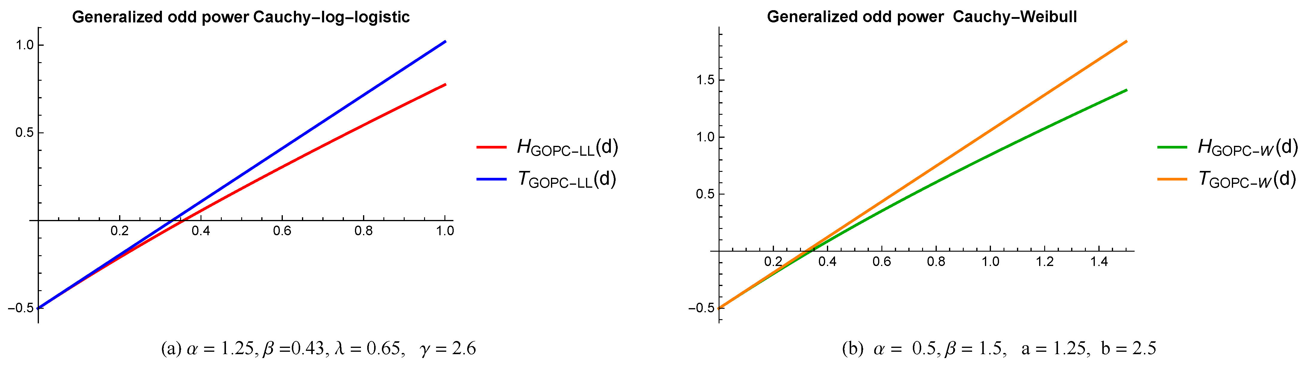
We consider two special cases of GOPC-G family with baseline distributions: Log-logistic and Weibull called GOPC-LL and GOPC-W, respectively. Figure 1 presents graphs of approximation functions H and T for fixed parameters in the cases of GOPC-LL and GOPC-W distributions.

The cumulative distribution function of log-logistic distribution is given by

$$G\left(t\right)=\frac{1}{1+{\left(\frac{t}{\lambda }\right)}^{-\gamma }},$$

where $t>0$, $\lambda >0$ and $\gamma >0$.

Definition 3.

Generalized odd power Cauchy-log-logistic (GOPC-LL) distribution is associated with the cumulative distribution function given as

$$F_{GOPC-LL}(t;\alpha ,\beta ,\lambda ,\gamma )=\frac{2}{\pi }arctan\left({\left(\frac{{\left(\frac{1}{{\left(\frac{t}{\lambda }\right)}^{-\gamma }+1}\right)}^{\alpha }}{1-{\left(\frac{1}{{\left(\frac{t}{\lambda }\right)}^{-\gamma }+1}\right)}^{\alpha }}\right)}^{\beta }\right).$$

(5)

Then for the one-sided Hausdorff approximation (using square unit ball with a side d) we have

$$F_{GOPC-LL}(t_0+d;\alpha ,\beta ,\lambda ,\gamma )=1-d,$$

(6)

where

$$F_{GOPC-LL}(t_0;\alpha ,\beta ,\lambda ,\gamma )=\frac{1}{2}\mathrm{with}{t}_0=\lambda {\left(\frac{2^{-1/\alpha }}{1-2^{-1/\alpha }}\right)}^{1/\gamma }.$$

Now we are ready to state our first corollary of Theorem 1. It shows how one-sided Hausdorff distance is related with parameters of cumulative distribution function.

Theorem 2.

Let

$$B=1+\frac{2\alpha \beta \gamma 2^{\frac{1}{\alpha }}{\left(2^{1/\alpha }-1\right)}^{1+\frac{1}{\gamma }}}{\pi \lambda }.$$

(7)

Then the one-sided Hausdorff distance d between interval Heaviside step function $h_{t_0}\left(t\right)$ and the cumulative distribution function $F_{GOPC-LL}(t;\alpha ,\beta ,\lambda ,\gamma )$ defined by (5) satisfies the following inequalities for $2.1B>e^{1.05}$:

$$d_l=\frac{1}{2.1B}<d<\frac{ln\left(2.1B\right)}{2.1B}=d_r.$$

Table 1. Bounds for Hausdorff distance d according to Theorem 2.

$\mathit{\alpha }$	$\mathit{\beta }$	$\mathit{\lambda }$	$\mathit{\gamma }$	${\mathit{d}}_{\mathit{l}}$	d computed by (6)	${\mathit{d}}_{\mathit{r}}$
1.05	5.71	0.01	2.23	0.001191	0.004766	0.008014
10.05	0.71	0.03	5.23	0.014494	0.045419	0.061356
2.51	7.06	2.16	13.13	0.029458	0.053603	0.103833
0.15	0.61	0.03	2.55	0.015408	0.059157	0.064296
2.71	9.31	0.12	0.91	0.058845	0.094795	0.166699

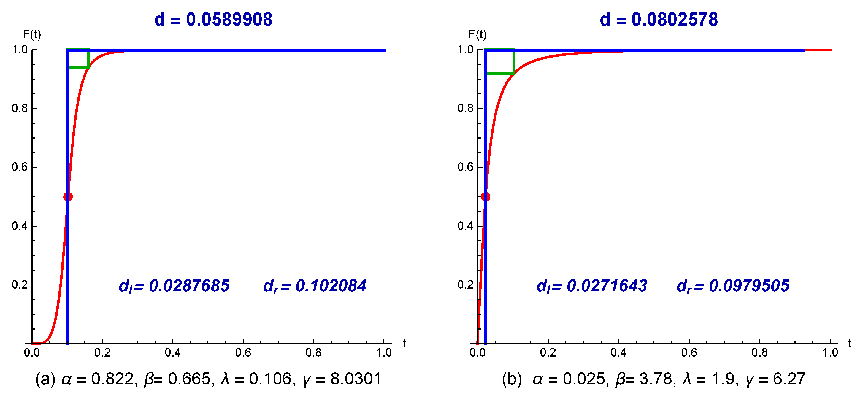
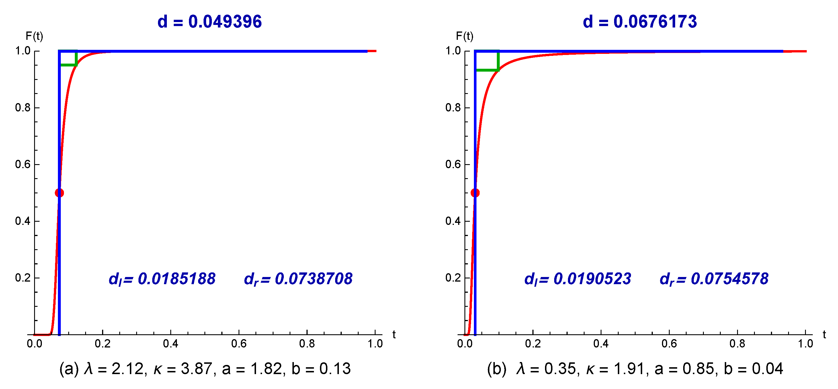
gives several numerical experiments for different values of parameters $\alpha$, $\beta$, $\lambda$ and $\gamma$. The values of estimates $d_l$ and $d_r$ are computed according to Theorem 2. Figure 2 shows some graphical representations.

Let us recall that the cumulative distribution function of Weibull distribution is

$$G\left(t\right)=1-e^w,$$

where $w=-{\left(\frac{t}{b}\right)}^a$, $a>0$ is a shape parameter and $b>0$ is a scale parameter.

Definition 4.

Generalized odd power Cauchy–Weibull (GOPC-W) distribution is associated with the cumulative distribution function given as

$$F_{GOPC-W}(t;\alpha ,\beta ,a,b)=\frac{2}{\pi }arctan{\left(\frac{{\left(1-e^{-{\left(\frac{t}{b}\right)}^a}\right)}^{\alpha }}{1-{\left(1-e^{-{\left(\frac{t}{b}\right)}^a}\right)}^{\alpha }}\right)}^{\beta }.$$

(8)

Here we examine the one-sided Hausdorff distance of the Heaviside step function and cumulative distribution function $F_{GOPC-W}(t;\alpha ,\beta ,a,b)$ defined by (8). For the “median level” we have

$$F_{GOPC-W}(t_0;\alpha ,\beta ,a,b)=\frac{1}{2}\mathrm{with}{t}_0=b\sqrt[a]{log\left(\frac{1}{1-2^{-1/\alpha }}\right)}.$$

Then the one-sided Hausdorff distance d satisfies the following nonlinear equation

$$F_{GOPC-W}(t_0+d;\alpha ,\beta ,a,b)=1-d.$$

(9)

Next corollary of Theorem 1 gives useful estimates for the one-sided Hausdorff approximation d.

Theorem 3.

Let

$$C=1+\frac{2a\alpha \beta \left(2^{1/\alpha }-1\right)log{\left(1+\frac{1}{2^{1/\alpha }-1}\right)}^{\frac{a-1}{a}}}{\pi b}.$$

(10)

Then the one-sided Hausdorff distance d between interval Heaviside step function $h_{t_0}\left(t\right)$ and the cumulative distribution function $F_{GOPC-W}(t;\alpha ,\beta ,a,b)$ defined by (8) satisfies the following inequalities for $2.1C>e^{1.05}$:

$$d_l=\frac{1}{2.1C}<d<\frac{ln\left(2.1C\right)}{2.1C}=d_r.$$

Table 2. Bounds for the one-sided Hausdorff distance d computed by Theorem 3.

$\mathit{\alpha }$	$\mathit{\beta }$	a	b	${\mathit{d}}_{\mathit{l}}$	d computed by (9)	${\mathit{d}}_{\mathit{r}}$
1.62	2.45	0.92	0.05	0.018521	0.042754	0.073878
0.85	0.93	1.75	0.09	0.044115	0.075925	0.137681
1.62	3.25	4.93	1.15	0.052857	0.080239	0.155409
3.09	0.93	2.82	0.25	0.059214	0.087407	0.167374
0.09	3.75	2.01	1.98	0.043054	0.099305	0.135419

presents some computational examples for different values of parameters $\alpha$, $\beta$, a and b. We exhibit the values of $d_l$ and $d_r$ as we use Theorem 3. Some graphical visualizations are given in Figure 3.

2.2. Some Special Models from Truncated Cauchy Power Odd Frechet-G Family of Distributions

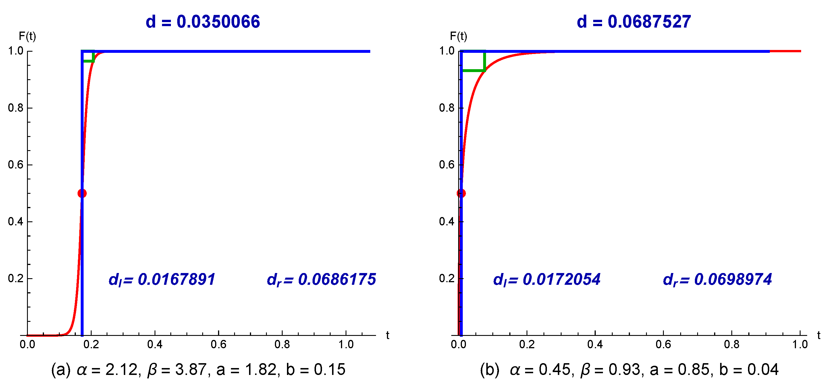
In this section we consider two submodels of TCPOF-G family based on the baseline distributions: Weibull and Lomax named TCPOFW and TCPOFL. For these two special cases, we obtain upper and lower estimates for the one-sided Hausdorff distance d. Since the proof of Theorems 4 and 5 follows the ideas given in Theorem 1, then they will be omitted. Some computational examples and graphical representations are presented in

Table 3. Bounds for one-sided Hausdorff distance d computed by Theorem 4.

$\mathit{\lambda }$	$\mathit{\kappa }$	a	b	${\mathit{d}}_{\mathit{l}}$	d computed by (12)	${\mathit{d}}_{\mathit{r}}$
0.29	3.87	1.82	0.13	0.012021	0.031634	0.053148
1.59	2.45	0.92	0.05	0.014215	0.040334	0.060465
0.05	2.32	1.02	0.18	0.020202	0.057339	0.078829
3.62	3.87	4.82	1.03	0.039285	0.071086	0.127163
1.62	3.25	4.93	1.15	0.050716	0.085735	0.151211

with Figure 4 for TCPOFW distribution and

Table 4. Bounds for the one-sided Hausdorff distance d computed by Theorem 5.

$\mathit{\lambda }$	$\mathit{\kappa }$	a	b	${\mathit{d}}_{\mathit{l}}$	d computed by (14)	${\mathit{d}}_{\mathit{r}}$
0.84	3.63	1.75	0.16	0.021236	0.055276	0.081803
0.05	2.32	1.02	0.18	0.024986	0.072125	0.092186
1.62	2.45	0.92	0.05	0.034049	0.087080	0.115085
1.62	3.25	4.93	1.15	0.049539	0.094769	0.148865
3.67	5.05	6.01	2.88	0.064591	0.109868	0.176961

with Figure 5 for TCPOFL distribution, respectively.

Definition 5.

Truncated Cauchy Power Odd Fréchet–Weibull (TCPOFW) distribution is associated with the cumulative distribution function given as

$$F_{TCPOFW}(t;\lambda ,\kappa ,a,b)=\frac{4}{\pi }arctan\left\{e^{-\lambda {\left(\frac{e^{-{\left(\frac{t}{b}\right)}^a}}{1-e^{-{\left(\frac{t}{b}\right)}^a}}\right)}^{\kappa }}\right\}.$$

(11)

Hence, the one-sided Hausdorff distance d between $F_{TCPOFW}(t;\lambda ,\kappa ,a,b)$ defined by (11) and the Heaviside function $h_{t_0}\left(t\right)$ satisfy the relation

$$F_{TCPOFW}(t_0+d;\lambda ,\kappa ,a,b)=1-d,$$

(12)

where

$$F_{TCPOFW}(t_0;\lambda ,\kappa ,a,b)=\frac{1}{2}\mathrm{with}{t}_0=b\left({log\left(1+{\lambda }^{1/\kappa }log{\left(cot\left(\frac{\pi }{8}\right)\right)}^{-1/\kappa }\right)}^{1/a}\right).$$

Theorem 4.

Let

$$D=1+\frac{\sqrt{2}a\kappa {\lambda }^{-1/\kappa }log\left(cot\left(\frac{\pi }{8}\right)\right)\left({\lambda }^{1/\kappa }+\sqrt[\kappa ]{log\left(cot\left(\frac{\pi }{8}\right)\right)}\right)log{\left(1+{\lambda }^{1/\kappa }log{\left(cot\left(\frac{\pi }{8}\right)\right)}^{-1/\kappa }\right)}^{\frac{a-1}{a}}}{\pi b}.$$

Then the one-sided Hausdorff distance d between interval Heaviside step function $h_{t_0}\left(t\right)$ and the cumulative distribution function $F_{TCPOFW}(t;\lambda ,\kappa ,a,b)$ defined by (11) satisfies the following inequalities for $2.1D>e^{1.05}$:

$$d_l=\frac{1}{2.1D}<d<\frac{ln\left(2.1D\right)}{2.1D}=d_r.$$

Definition 6.

Truncated Cauchy Power Odd Fréchet–Lomax (TCPOFL) distribution is associated with the cumulative distribution function given as

$$F_{TCPOFW}(t;\lambda ,\kappa ,a,b)=\frac{4}{\pi }arctan\left\{e^{-\lambda {\left(\frac{{\left(1+\frac{t}{b}\right)}^{-a}}{1-{\left(1+\frac{t}{b}\right)}^{-a}}\right)}^{\kappa }}\right\}.$$

(13)

The one-sided Hausdorff distance d between $F_{TCPOFL}(t;\lambda ,\kappa ,a,b)$ defined by (13) and the Heaviside function $h_{t_0}\left(t\right)$ satisfies the relation

$$F_{TCPOFL}(t_0+d;\lambda ,\kappa ,a,b)=1-d,$$

(14)

where

$$F_{TCPOFL}(t_0;\lambda ,\kappa ,a,b)=\frac{1}{2}\mathrm{with}{t}_0=b\left({\left(1+{\lambda }^{1/\kappa }log{\left(cot\left(\frac{\pi }{8}\right)\right)}^{-1/\kappa }\right)}^{1/a}-1\right).$$

Theorem 5.

Let

$$E=1+\frac{\sqrt{2}a\kappa {\lambda }^{-1/\kappa }log{\left(cot\left(\frac{\pi }{8}\right)\right)}^{\frac{\kappa +1}{\kappa }}{\left(1+{\lambda }^{1/\kappa }log{\left(cot\left(\frac{\pi }{8}\right)\right)}^{-1/\kappa }\right)}^{\frac{a-1}{a}}}{\pi b}.$$

Then the one-sided Hausdorff distance d between interval Heaviside step function $h_{t_0}\left(t\right)$ and the cumulative distribution function $F_{TCPOFL}(t;\lambda ,\kappa ,a,b)$ defined by (13) satisfies the following inequalities for $2.1E>e^{1.05}$:

$$d_l=\frac{1}{2.1E}<d<\frac{ln\left(2.1E\right)}{2.1E}=d_r.$$

2.3. Some Applications

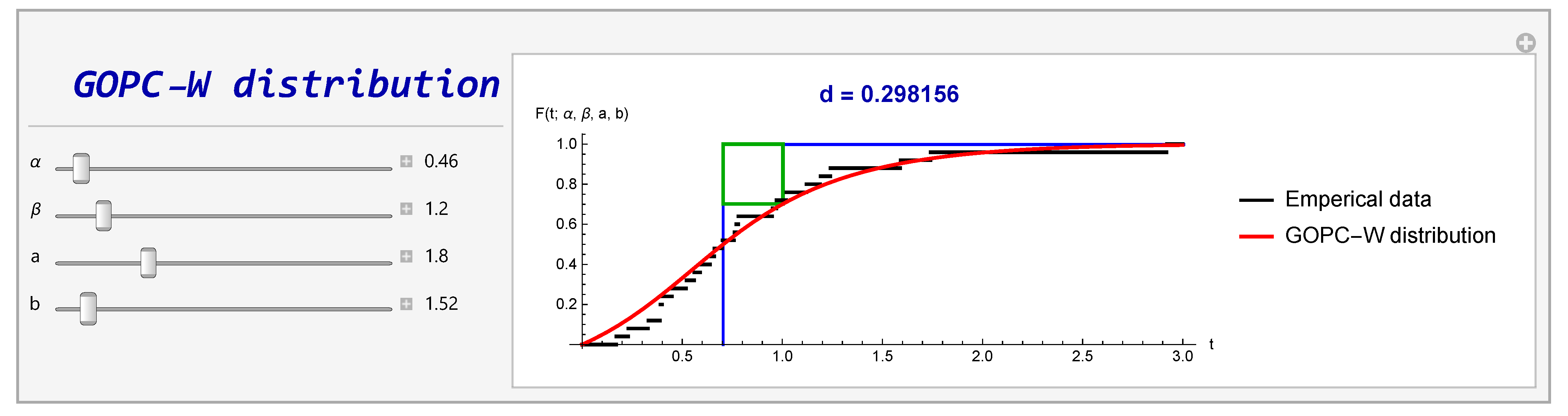
In this section we present one particular application of obtained results. We consider data that represent runoff amounts of Jug Bridge, Maryland (see Chhikara and Folks [23]):

$$\begin{array}{ccc}& & 0.17,1.19,0.23,0.33,0.39,0.39,0.40,0.45,0.52,0.56,0.59,0.64,0.66\hfill \\ & & 0.70,0.76,0.77,0.78,0.95,0.97,1.02,1.12,1.24,1.59,1.74,2.92.\hfill \end{array}$$

Here we present a simple dynamic programming module, implemented within the programming environment CAS Wolfram Mathematica, for the analysis of cumulative distribution function of GOPC-W (see Figure 6). We consider that the considered data set can be approximated with cumulative distribution function GOPC-W $F(t;\alpha ,\beta ,a,b)$ with parameters $\alpha =0.46$, $\beta =1.2$, $a=1.8$ and $b=1.52$. We compute Hausdorff distance with its upper and lower estimates as we use Theorem 3. The obtained values are $d=0.298156$ with estimates $d_l=0.266013$ and $d_r=0.352257$, respectively. Our module provides graphical visualization of the results. Similar modules can be obtained for other cases of proposed families.

2.4. Simple Comparison of GOPC-G and TCPOF-G Families

Some special cases of GOPC-G family and TCPOF-G family are proposed from [6] and [7], respectively. Reader can obtain many others using different base cumulative distribution functions. For example in the literature there are many modifications of classical Weibull distribution. In 2014, Almalki and Nadarajah [24] present a review of some of them.

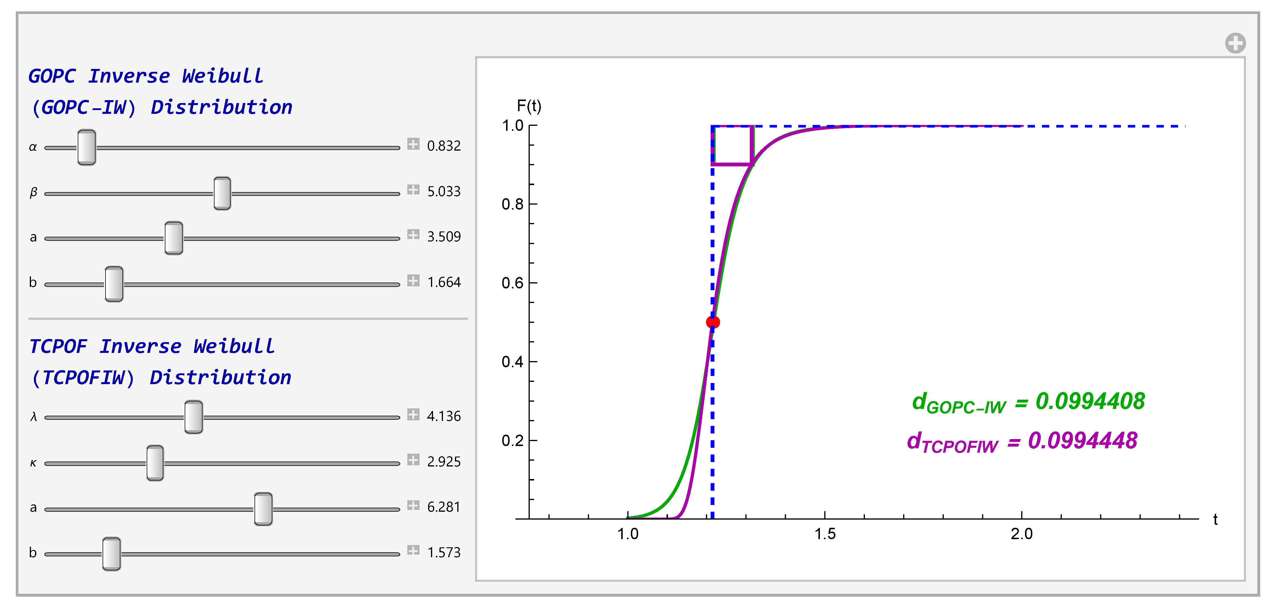
In this section we propose a simple comparison of GOPC-G and TCPOF-G families with the same Weibull-type correction. Let us consider an example with Inverse Weibull distribution with cumulative distribution function defined by

$$G\left(t\right)=e^{-b{t}^{-a}}.$$

Hence we obtain the following submodels of GOPC-G and TCPOF-G named GOPC-IW and TCPOFIW, respectively.

Cumulative distribution function of Generalized odd power Cauchy-Inverse Weibull (GOPC-IW) distribution is defined by

$$F_{GOPC-IW}(t;\alpha ,\beta ,a,b)=\frac{2}{\pi }arctan{\left(\frac{{\left(e^{-b{t}^{-a}}\right)}^{\alpha }}{1-{\left(e^{-b{t}^{-a}}\right)}^{\alpha }}\right)}^{\beta }.$$

(15)

Cumulative distribution of Truncated Cauchy Power Odd Fréchet-Inverse Weibull (TCPOFIW) distribution is given by

$$F_{TCPOFIW}(t;\lambda ,\kappa ,a,b)=\frac{4}{\pi }arctan\left\{e^{-\lambda {\left(\frac{1-e^{-b{t}^{-a}}}{e^{-b{t}^{-a}}}\right)}^{\kappa }}\right\}.$$

(16)

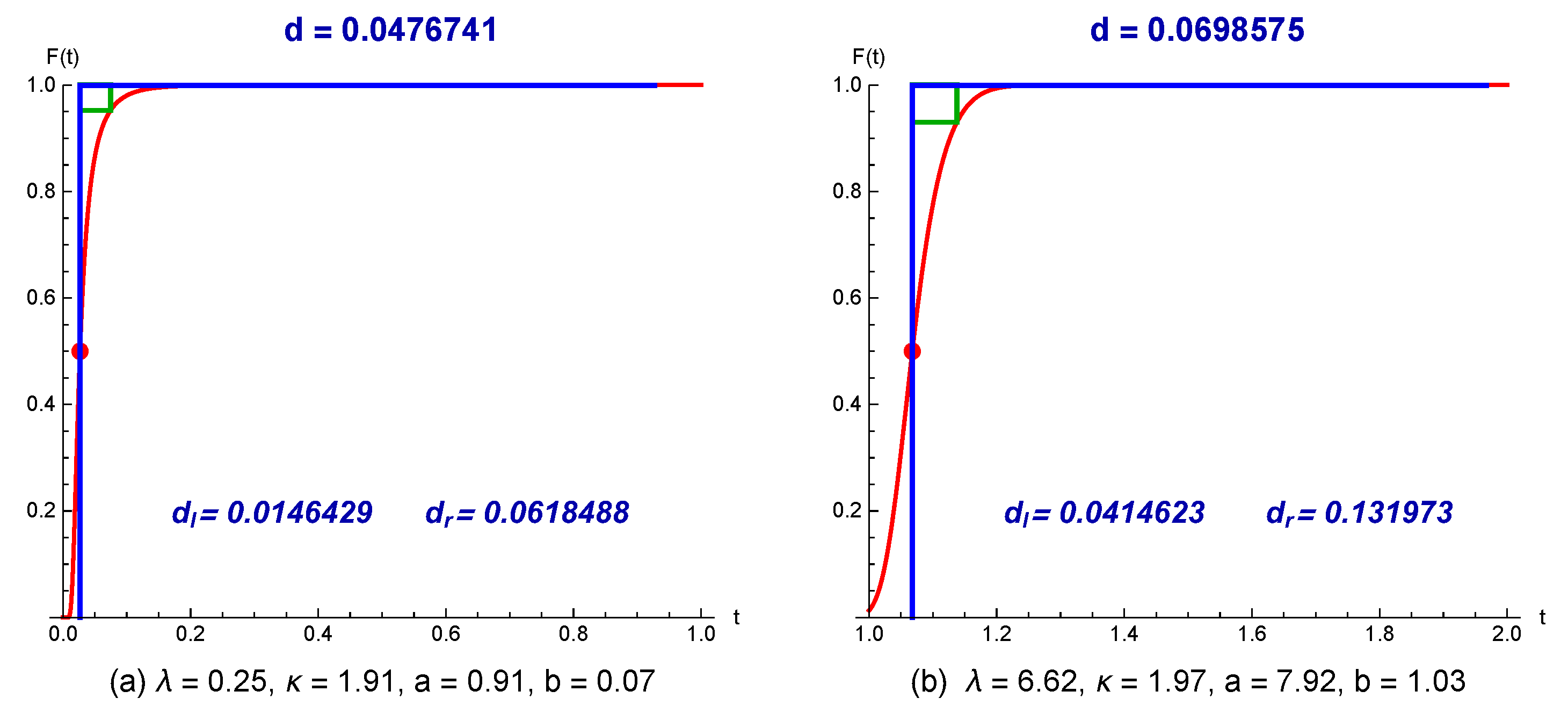
In Figure 7, we present simple comparatively investigation of asymptotic behavior of one-sided Hausdorff distance between Heaviside step function and cumulative distribution functions of GOPC-IW and TCPOFIW. Both models are based on arctangent function but they have different construction. In our simple dynamic programming module we choose corresponding distribution parameters which yield similar type of cumulative shapes. The corresponding Hausdorff distances that we obtain are $d_{GOPC-IW}=0.0994408$ and $d_{TCPOFIW}=0.0994448$.

3. Recurrent Generation of New Families of “Adaptive Functions”

We construct a family of recurrence generated activation functions based on GOPC-G family in the following way

$$F_{i+1}\left(t\right)=\frac{2}{\pi }arctan\left\{{\left[\frac{G{(t+F_i\left(t\right);\xi )}^{\alpha }}{1-G{(t+F_i\left(t\right);\xi )}^{\alpha }}\right]}^{\beta }\right\},i=0,1,2,\dots ,$$

(17)

with

$$F_0\left(t\right)=F_{GOPC-G}(t;\alpha ,\beta ,\xi );F_0\left(0\right)=0.$$

The reader may formulate some special cases of a family of recurrence generated activation functions with the corresponding approximation problems based on GOPC-G family or TCPOF-G family. In this section we consider a special case based on GOPC-G family with Weibull as baseline distribution. Here we investigate the one-sided Hausdorff approximation of the shifted Heaviside function by means of the corresponding family at “median level”. For other results about families of recurrence generated parametric activation functions with various approximation and modeling aspects see [12,14,17,18,22].

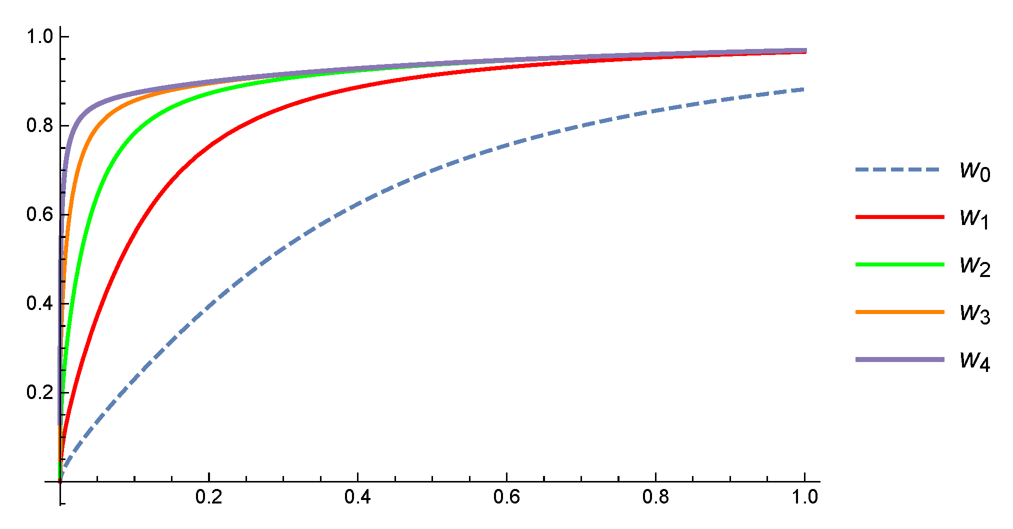
Let us consider one special case. The recurrent family based on GOPC-W is defined by

$$w_{i+1}\left(t\right)=\frac{2}{\pi }arctan{\left(\frac{{\left(1-e^{-{\left(\frac{t+w_i\left(t\right)}{b}\right)}^a}\right)}^{\alpha }}{1-{\left(1-e^{-{\left(\frac{t+w_i\left(t\right)}{b}\right)}^a}\right)}^{\alpha }}\right)}^{\beta },i=0,1,2,\dots ,$$

(18)

with

$$w_0\left(t\right)=\frac{2}{\pi }arctan{\left(\frac{{\left(1-e^{-{\left(\frac{t}{b}\right)}^a}\right)}^{\alpha }}{1-{\left(1-e^{-{\left(\frac{t}{b}\right)}^a}\right)}^{\alpha }}\right)}^{\beta };w_0\left(0\right)=0.$$

The recurrence generated functions $w_0\left(t\right)$, $w_1\left(t\right)$, $w_2\left(t\right)$, $w_3\left(t\right)$ and $w_4\left(t\right)$ from family (18) for fixed $\alpha =0.25$, $\beta =1.75$, $a=1.25$ and $b=2.5$ are visualized on Figure 8.

The one-sided Hausdorff distance d between cumulative distribution function $w_i\left(t\right)$$i=1,2,\dots$ and the Heaviside function $h_{t_0}\left(t\right)$ satisfies the following nonlinear equation

$$w_i(t_0+d)=1-d,$$

(19)

where $t_0$ is a positive solution of the equation ${\displaystyle w_i\left(t_0\right)=\frac{1}{2}}$. We present some computational examples in

Table 5. The one-sided Hausdorff distance d computed by (19) for reccurent family (18).

	$\mathit{\alpha }=0.25$, $\mathit{\beta }=1.51$	$\mathit{\alpha }=0.09$, $\mathit{\beta }=0.30$	$\mathit{\alpha }=0.41$, $\mathit{\beta }=0.98$	$\mathit{\alpha }=1.20$, $\mathit{\beta }=3.50$	$\mathit{\alpha }=0.75$, $\mathit{\beta }=3.80$
	$\mathit{a}=1.25$, $\mathit{b}=1.75$	$\mathit{a}=2.90$, $\mathit{b}=0.60$	$\mathit{a}=1.30$, $\mathit{b}=0.70$	$\mathit{a}=0.20$, $\mathit{b}=0.20$	$\mathit{a}=0.25$, $\mathit{b}=1.90$
$w_0$	0.253906	0.338647	0.249528	0.167576	0.203568
$w_1$	0.154401	0.170627	0.148968	0.063312	0.098448
$w_2$	0.107709	0.113641	0.097871	0.033868	0.061280
$w_3$	0.089594	0.093047	0.073675	0.029762	0.052952
$w_4$	0.085553	0.085846	0.066701	0.029554	0.052124

. We show the asymptotic behavior of the one-sided Hausdorff distance for cumulative distribution functions $w_i\left(t\right)$, $i=1,2,\dots$ for different values of parameters $\alpha$, $\beta$, a and b. From these results, one can observe that how deeper we go into the recursion, the one-sided Hausdorff distance comes smaller.

4. Conclusions

The aim of this research is to study the asymptotic behavior of the one-sided Hausdorff distance between Heaviside step function and some cumulative distribution functions based on arctangent function and some baseline distribution. Estimates for the searching Hausdorff approximation are given. In practice, they can be used as one more possible criterion in examination of the one-sided Hausdorff approximation. Simple comparatively investigation of asymptotic behavior of one-sided Hausdorff distance between Heaviside step function and cumulative distribution functions of GOPC-G and TCPOF-G families with the same Weibull-type correction is presented. Moreover, we construct families of recurrence generated adaptive functions. One can formulate corresponding tasks with approximation problems using proposed methods for other families containing arctangent function and their extensions. In this way the researcher receive a lot of opportunities when choosing the appropriate model for approximation of cumulative specific data. We propose a simple dynamic software module that demonstrate how new results can be using with real cumulative data.

References

- Cordeiro, G.M.; Alizadeh, M.; Ramires, T.G.; Ortega, E.M. The generalized odd half-Cauchy family of distributions properties and applications. Commun. Stat. Theory Methods 2017, 46, 5685–5705. [Google Scholar]
- Alizadeh, M.; Altun, E.; Cordeiro, G.M.; Rasekhi, M. The odd power Cauchy family of distributions: Properties, regression models and applications. J. Stat. Comput. Simul. 2018, 88, 785–807. [Google Scholar]
- Aldahlan, M.A.; Jamal, F.; Chesneau, C.; Elgarhy, M.; Elbatal, I. The truncated Cauchy power family of distributions with inference and applications. Entropy 2020, 22, 346. [Google Scholar]
- Chakraburty, S.; Alizadeh, M.; Handique, L.; Altun, E.; Hamedani, G.G. A new extension of Odd Half-Cauchy family of distributions: Properties and applications with regression modeling. Stat. Transit. New Ser. 2021, 22, 77–100. [Google Scholar]
- Alkhairy, I.; Nagy, M.; Muse, A.H.; Hussam, E. The Arctan-X family of distributions: Properties, simulation, and applications to actuarial sciences. Complexity 2021, 14, 4689010. [Google Scholar]
- Altun, E.; Alizadeh, M.; Ramires, T.; Ortega, E. Generalized odd power Cauchy family and its associated heteroscedastic regression model. Stat. Optim. Inf. Comput. 2021, 3, 516–528. [Google Scholar]
- Shrahili, M.; Elbatal, I. Truncated Cauchy power odd Fréchet-G family of distributions: Theory and applications. Complexity 2021, 9, 4256945. [Google Scholar]
- Hausdorff, F. Set Theory, 2nd ed.; Chelsea Publication: New York, NY, USA, 1962. [Google Scholar]
- Sendov, B.L. Hausdorff approximations. In Mathematics and Its Applications; Springer Science & Business Media: Berlin/Heidelberg, Germany, 1990; Volume 50, pp. 1–367. [Google Scholar]
- Kyurkchiev, N. On the approximation of the step function by some cumulative distribution functions. Comp. Rend. Acad. Bulg. Sci. 2015, 68, 1475–1482. [Google Scholar]
- Kyurkchiev, N.; Iliev, A. On the Hausdorff distance between the Heaviside function and some Transmuted activation functions. Math. Model. Anal. 2016, 1, 8–12. [Google Scholar]
- Kyurkchiev, N.; Rahneva, O.; Iliev, A.; Malinova, A.; Rahnev, A. Investigations on Some Generalized Trigonometric Distributions. Properties and Applications; Plovdiv University Press: Plovdiv, Bulgaria, 2021; ISBN 978-619-7663-01-3. [Google Scholar]
- Kyurkchiev, N.; Iliev, A.; Rahnev, A. A new Cos-G family with baseline cumulative function of Volmer–type. Applications. Int. J. Pure Appl. Math. 2021, 15, 55–65. [Google Scholar]
- Kyurkchiev, N.; Pavlov, N.; Iliev, A.; Rahneva, O. Some classes of “Transmuted adaptive functions”. Applications. Commun. Appl. Anal. 2021, 25, 53–65. [Google Scholar]
- Kyurkchiev, N.; Iliev, A.; Arnaudova, V.; Rahnev, A. Investigation on some new cumulative distributions via Cosine and Sine functions. Int. J. Differ. Equ. Appl. 2021, 20, 75–88. [Google Scholar]
- Kyurkchiev, N.; Rahneva, O.; Malinova, A.; Iliev, A. On some adaptive G-families. Applications. Int. J. Differ. Equ. Appl. 2021, 20, 89–101. [Google Scholar]
- Kyurkchiev, N.; Iliev, A.; Rahneva, O.; Kyurkchiev, V. A look at some Trigonometric-G families baseline inverted exponential (cdf). Applications. Int. J. Differ. Equ. Appl. 2021, 20, 103–119. [Google Scholar]
- Kyurkchiev, N.; Iliev, A.; Rahnev, A. Properties and applications of a Tan–G family of “Adaptive functions”. Int. J. Circuits Syst. Signal Process. 2021, 15, 1292–1296. [Google Scholar]
- Kyurkchiev, N. Some intrinsic properties of Tadmor–Tanner functions: Related problems and possible applications. Mathematics 2020, 8, 1963. [Google Scholar]
- Vasileva, M. Some notes on the Omega distribution and the Pliant probability distribution family. Algorithms 2020, 13, 324. [Google Scholar]
- Vasileva, M.; Iliev, A.; Rahnev, A.; Kyurkchiev, K. On the approximation of the Haar scaling function by sigmoidal scaling functions. Int. J. Differ. Equ. Appl. 2021, 20, 1–13. [Google Scholar]
- Vasileva, M.; Rahneva, O.; Malinova, A.; Arnaudova, V. The odd Weibull-Topp-Leone-G power series family of distributions. Int. J. Differ. Equ. Appl. 2021, 20, 43–58. [Google Scholar]
- Chhikara, R.S.; Folks, J.L. The inverse Gaussian distribution as a lifetime model. Technometrics 1977, 19, 461–468. [Google Scholar]
- Almalki, S.J.; Nadarajah, S. Modifications of the Weibull distribution: A review. Reliab. Eng. Syst. Saf. 2014, 124, 32–55. [Google Scholar]
Figure 1.
Graph of functions and in the cases of GOPC-LL and GOPC-W distributions.
Figure 2.
Approximation of CDF function of GOPC-LL distribution.
Figure 3.
Approximation of CDF function of GOPC-W distribution.
Figure 4.
Approximation of CDF function of TCPOFW distribution.
Figure 5.
Approximation of CDF function of TCPOFL distribution.
Figure 6.
The model (8) for runoff amounts data (normalized) of Jug Bridge, Maryland.
Figure 7.
Hausdorff approximation of GOPC-IW and TCPOFIW distributions.
Figure 8.
The graphics of recurrence generated adaptive functions from family (18).