1. Introduction
Convolutional neural networks (CNNs) [
1] have arrived to stay. Since this kind of network has been generated, they have resolved multiple problems in different fields. In addition, they have demonstrated an excellent performance in computer vision tasks, for example, detection [
2,
3], segmentation [
4,
5,
6], and classification [
7,
8,
9], in different kinds of images. Nevertheless, when we work with medical imaging, we face a challenging problem related to different causes due to the lack of data for training, generalization problems, and others. Indeed, computer vision for medical purposes needs to be contextualized and related to the field of application. In other words, methods used to support medical decisions need to be considered as decision support tools, not mere computer science algorithms [
10]. For those reasons, the development of such tools needs to not only be a transposition of existing procedures, but be seen as a real, cyclic problem-solving issue [
11].
The first question that needs to be asked when applying interactive planning and cyclic problem solving is the representation of the observed reality. Nowadays, many different CNN architectures are used in medical image classification, such as InceptionV3 [
12], ResNets [
13], EfficientNets [
14], DenseNets [
15], MobileNetV2 [
16], and even the VGGNets [
17]. To the best of our knowledge, those methods follow computer science vision but make the abstraction of main practical needs, such as data availability and conditions of use. Moreover, the literature generates good solutions to classify medical images; however, they require high computing power, which implies that these types of solutions cannot be implemented in health centers with few computing resources [
18,
19]. Indeed, those methods make, in general, the abstraction of computational effort limitations and assume all users can meet the settings used to deploy the proposed algorithms, in terms of both hardware and of software. Due to public budgetary limitations in some countries, not all computational power can be met. Concerning data availability, not all countries have an extensive local database of images that would allow training and validating the proposed algorithms. To deal with this issue, two different public datasets of chest X-rays (CXRs), CheXpert [
20] and ChestX-ray14 [
21], can be used.
Given those issues, the aim of this paper was to propose and validate a transfer methodology based on CNNs for supporting medical decisions in CXR analysis for an application in the medical sector of Chile and South America. In this research, we used a dataset of 16,372 images of five different categories of common lung diseases, extracted from the images in references [
20,
21], i.e., atelectasis, cardiomegaly, consolidation, edema, and pleural effusion. The main purpose of the algorithm was to support medical diagnosis, so the reduction of false negative diagnoses gives medical staff a basis of pre-selected positive cases for which a decision concerning the final diagnosis and the consequent care needs to be taken. A multi-class classification problem was defined and processed with a CNN algorithm combined with transfer learning. Besides, for the classification purpose, we used the VGG16 [
17] architecture and made modifications to the last layers.
Section 2 describes the materials and the method used for this work. In
Section 3, we described the computational results with the test set. Finally, in
Section 4, we disclosed our conclusions and some future work about this research.
2. Materials and Methods
Medical image classification englobes a key set of methods and techniques for computer-aided diagnosis (CAD) systems. Traditional methods rely mainly on identifying the shape, color, and/or texture features of an image, as well as their combinations, and compare them to a basis (in general a database), representing characteristic images of a disease. Most medical image classification methods are problem-specific and have shown to be complementary to medical diagnosis decisions. However, the complexity and the diversity of decisions and resources make the decisions difficult while relying only on image classification. For those reasons, the proposed methodology aims to develop a medical image classification method, which is not only for top-down or bottom-up computing and algorithmic vision, but from a problem-solving and decision-support perspective.
Therefore, the proposed methodological framework follows cyclic problem-solving vision [
10]. Indeed, since the objective of the algorithms is to develop a need to support decisions in medical disease identification, an interactive planning methodology to solve issues from operations research seems suitable. In interactive planning, the following elements need to be considered [
22,
23]:
Ends or objectives: in the present work, the objective was to support medical diagnosis by classifying X-ray images in order to pre-assign a disease type;
Means: intended as policies, programs, projects, practices, and courses of action to be taken. This includes medicine manpower competencies and hospital/medical center organizational issues;
Resources: intended as physical, material, and information resources. Since the research was conducted for an application in Chile, it is important to consider that the proposed tool needs to use open data to be constructed and there are not available national databases. Thus, affordable hardware needs to be able to use the tool, in order to be potentially deployed across the country;
The two last elements, i.e., implementation and control, were not considered here, although the abovementioned implementation issues have been taken into account when dealing with resource specifications.
Taking into account those elements and the problem-solving cycle of Ackoff [
10], discussed and extended in [
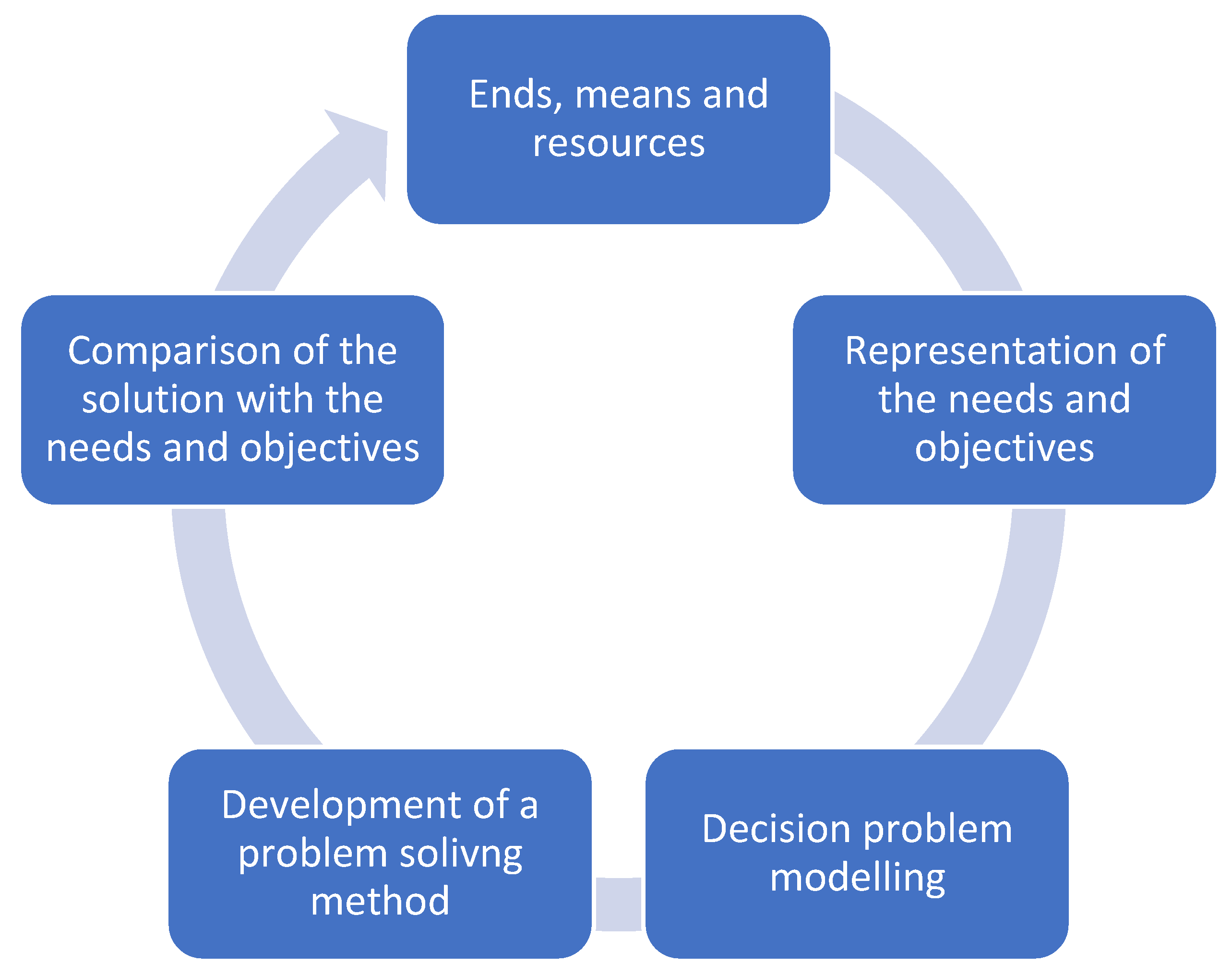
24], the general methodology followed here is related to the chart below (
Figure 1). It is presented as a cyclic procedure instead of the classical, iterative one [
11,
24].
The chart shows that, taking into account ends, means, and resources, a cyclic procedure starting from the definition of the first problem is needed. Once the problem is defined, a solution method needs to be implemented, which should be applicable with the needs and resources available. Once a solution is found, it needs to be confronted with the ends of the stakeholders, until the given problem and method allow responding satisfactorily to the ends while using the available resources and means in an efficient way. Here, the ends are to support medical decisions in a resource-constrained context of developing countries, which means computation capabilities are lower than those of developed countries with highly advanced research centers. Moreover, decision support implies that it is the final decision-maker that decides the computer-based tool, giving a set of elements and solutions to support the decision but not taking the decision at his or her place. In other words, the main aim of the proposed tool (ends) is not to provide an exact classification and a choice of diseases given an image, but provide, for each image, a correspondence to the most probable disease it could belongs to, the final medical decision on the disease being made by the medical staff analyzing it on the basis of their knowledge and experience, and the classification being then a support to guide decisions, but not a substitute to the medical capabilities. For all those reasons, the methodology for the construction of the proposed decision-support framework is organized in eight phases:
Definition of the decision problem;
Selection of databases for the algorithm construction and calibration: the first step of the methodology is an analysis of available X-ray image databases, which are both open and have already been used for image identification, in order to facilitate having standards and baselines when developing the algorithm;
Random sampling: from the selected databases, a random sampling procedure is used to select a set of data for algorithm construction purposes;
Sample analysis: After selecting the sample, it needs to be analyzed to examine the suitability and identify different aspects for preprocessing the purpose for algorithm construction;
Image preprocessing: after the analysis of the sample, different standardizations are applied to each image as pixel normalization between 0 and 255.0 and resized to 150 × 150 pixels;
CNN programing, transfer learning, and CNN modifications, to first construct an algorithm and then improve it;
CNN training on the selected image databases;
CNN testing and analysis of the computational results.
2.1. Definition of the Decision Problem
Given the considerations presented above, the main decision problem is to choose which disease is the most suitable given a set of images of a patient, with respect to those of a training database. As mentioned above, those methods are, in general, dependent on problems and constructed/calibrated for a specific disease identification. The chosen field was CXR identification for two main reasons. The first is that major image databases exist and can be used to develop and train algorithms to compare the proposed algorithm’s performance with those of previous works in the same field. However, data availability is not a sufficient condition to motivate our choice. Therefore, the second reason is from the perspective of the potential and needs of application of X-ray imagery: starting from developing countries needs and having university contacts with Chilean health system stakeholders, it appears that X-ray imaging is one of the main fields of application of computer vision that would add an important contribution to medical decision making. Moreover, the means of the medical healthcare system need to be considered when developing the decision-support method and then the image classification algorithm. Therefore, it seems important to explain here what we intend to do by decision support, since this definition conditions the accuracy requirements and the error acceptances of the algorithm: decision support is the proposal of elements for the decision maker to take the decision. In the medical field, this means that the algorithm gives a probability that the disease corresponds to a given one, but it depends on the medical care professional to make a final decision. The main decisions will then arise based on two main elements:
The choice of the number of zone categories is given by the number of possible diseases. This assumes that no unknown disease is considered, indicating diseases other than those of the initial category classification are used to train the algorithm;
The exact assignment of a disease to a category is impossible, since medical decisions made by humans are not infallible. Instead, probable correspondences can be used to make the decision maker reflect and find the most suitable assignment, on the basis of medical thinking, not only on that of an image correspondence. Moreover, the decision support method needs to be run on standard computing hardware, which implies a decrease of accuracy and an increase of computational time. For those reasons, high accuracy errors can be accepted.
Two main ways of making that classification can be defined are as following: the first is multi-label classification, in which each image can be associated to one or more diseases. The second is mono-label multiple category assignment, in which each image is associated to only one disease. Although the first is the most popular in CXR imaging (almost all works deal with it), it presents two main limitations of our present research: the first is resource consumption, which is much higher by the need of managing multiple layers in parallel, so the second method seems more suitable to be implemented in hardware. A second issue, which is more on a system-thinking and problem-solving viewpoint [
25,
26], is that multi-label algorithms assign different diseases to a single image, so they are not aimed at identifying the exact disease, but at showing if the image represents an ill chest or a good wealth one (in other words, the medical staff needs in any case to examine the image to make a decision). We can then obtain a similar result with a single assignment algorithm, because since it identifies a disease, even not the correct one, the final result is the same if it is able to identify an ill chest and distinguish it from a good health one but the computational efforts are reduced.
Consequently, the problem can be seen as a minimum dissimilarity-matching problem. In other words, given image j defined by a set of pixels characterizing its geometric form, shape, colour, texture (by defining an intensity, a brightness, etc.), and a database of medical images representing a set S = S1 … Si … Sn of diseases, the problem is to assign image j to disease Si that minimizes the dissimilarities between this image and all the images I = 1 … k of the disease set Si, with each dissimilarity (shape, colour, and texture) being defined by a set of distances between the values of the given image and those of the images of the reference database.
2.2. Databases Selection
To generate the database used for this work, we used public datasets [
20,
21]. One of the main reasons of this choice was the quantity of images available from each one of them. Besides, these two datasets contain image data from different common lung diseases, because one of the main death causes in Chile is the lungs disease [
27].
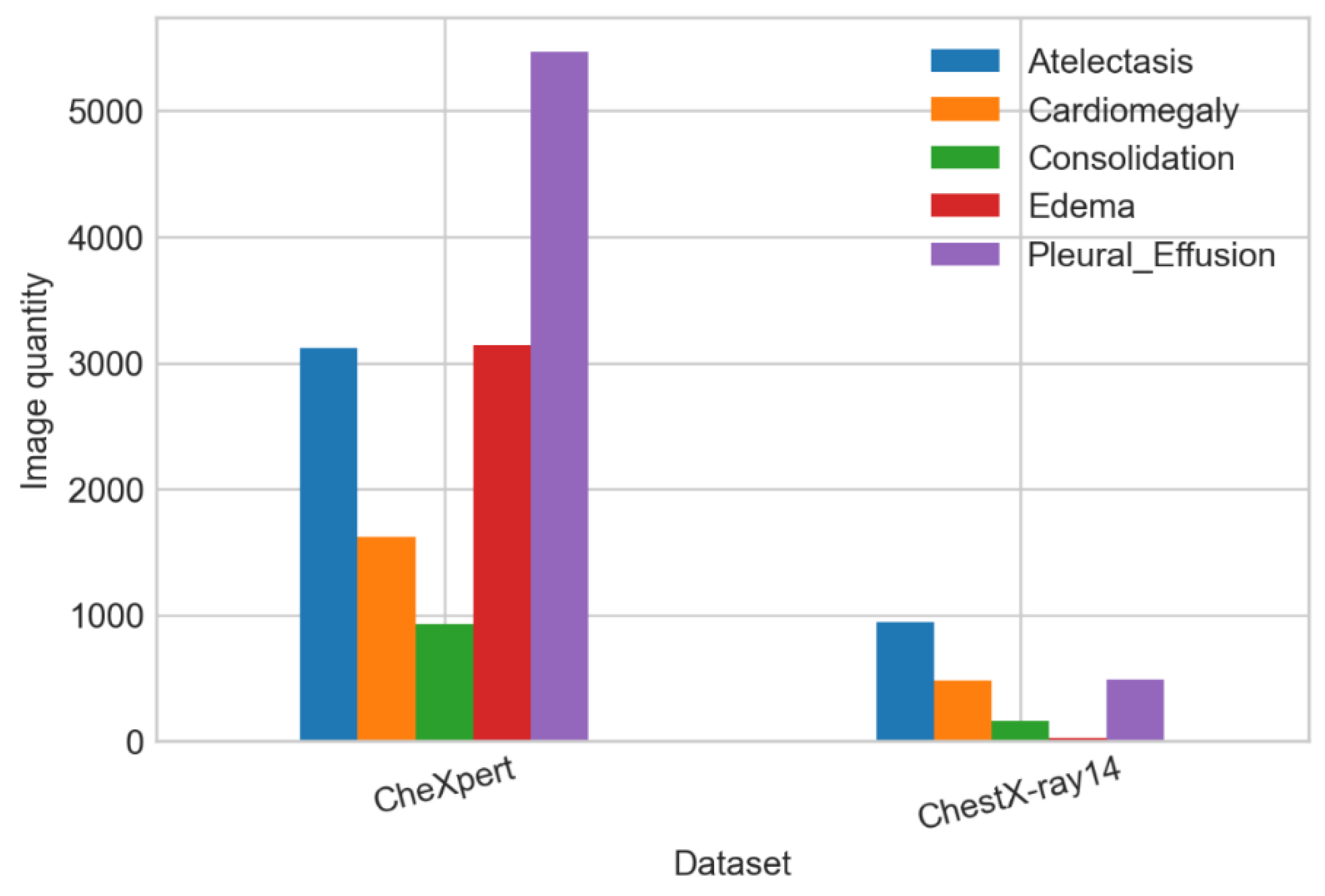
In
Table 1, we can see the image quantity used for each category from different datasets. We constructed the first database of 16,372 images by combining all images available. We observed the most common disease (in the number of images) is pleural effusion, with almost 6000 images, and the least common is consolidation, with only 1086. This makes the heterogeneity of the population of images in terms of frequency (
Figure 2). Thus, a sampling procedure is required to adjust that frequency to a homogeneous one.
2.3. Random Sampling
After the dataset generation, we took a random sample of 1086 images per category for the purpose of balancing every category with the same number of images (
Figure 1). Since all diseases are similar statistically and can be considered as internally homogeneous, a simple random sampling without replacement was chosen. The size of the sample was set to the minimum size of all 5 categories in order to have the maximum size of the sample without the need of replacement. Consequently, we dealt with a balanced classification problem, since all categories of the sample had the same characteristics.
2.4. Sample Analysis
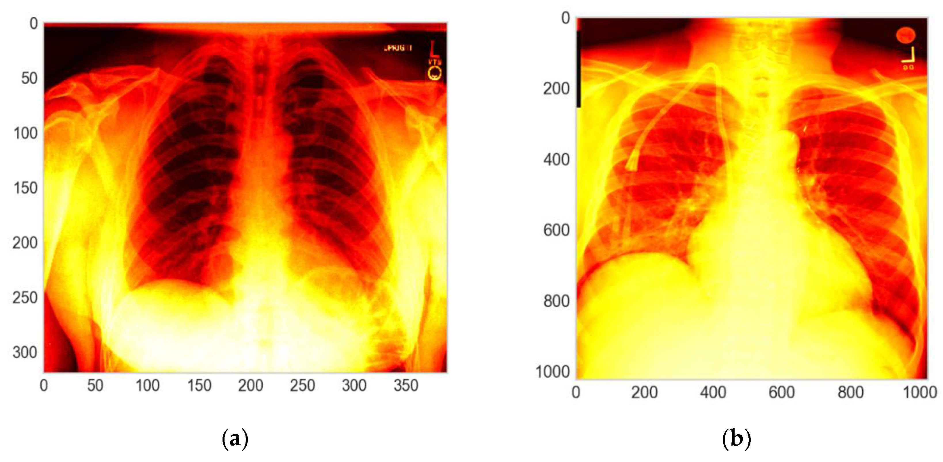
With the objective of identifying the differences between the images in [
20,
21], we developed an exploratory data analysis (EDA). The main actions of the EDA were the identification of the images’ dimensions (mainly height and width) as well as the color scales of the images. Thus, the main metrics used for the EDA were the height and the width of each image and then the representation of the greyscales or color scales on a standard basis.
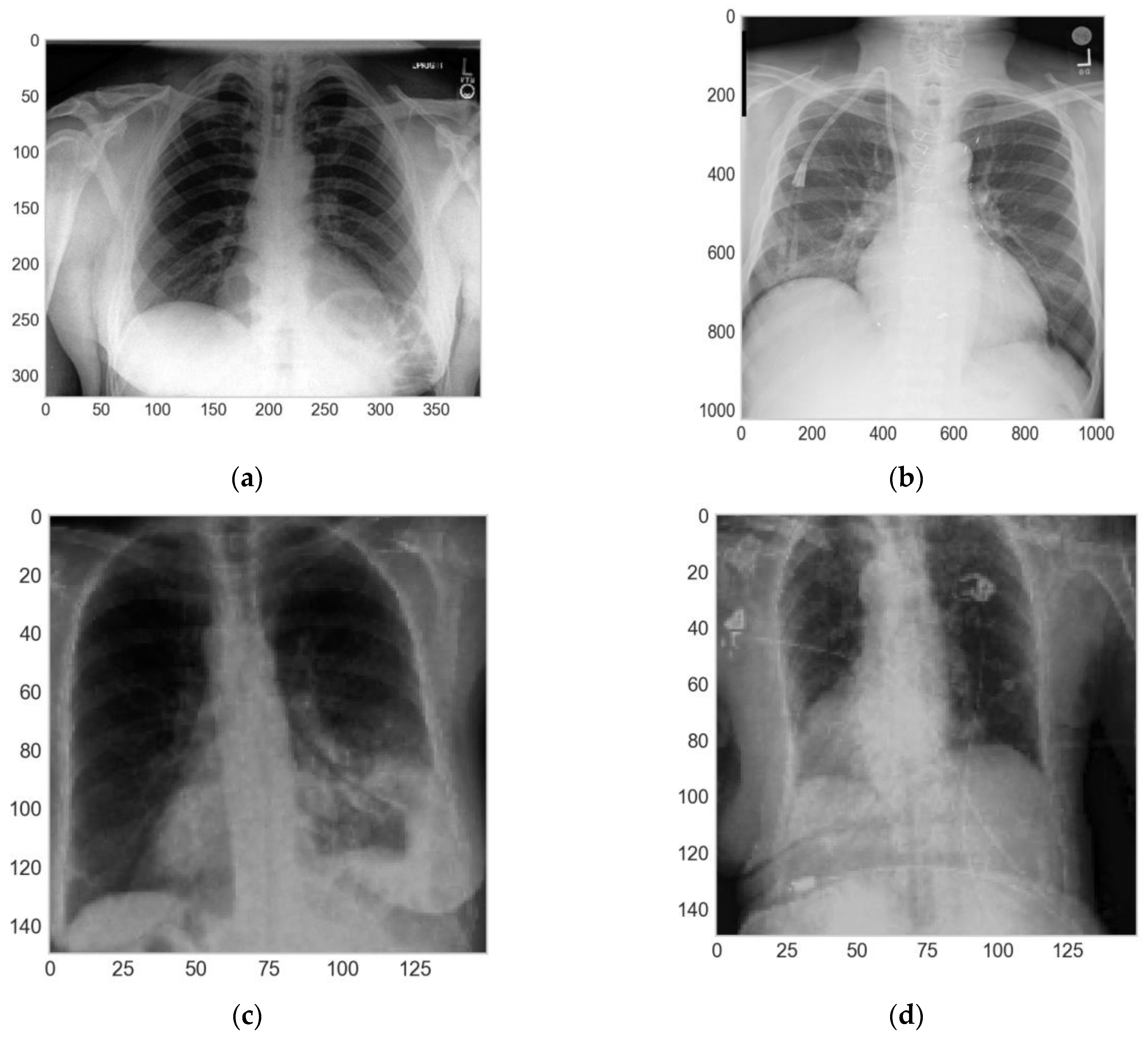
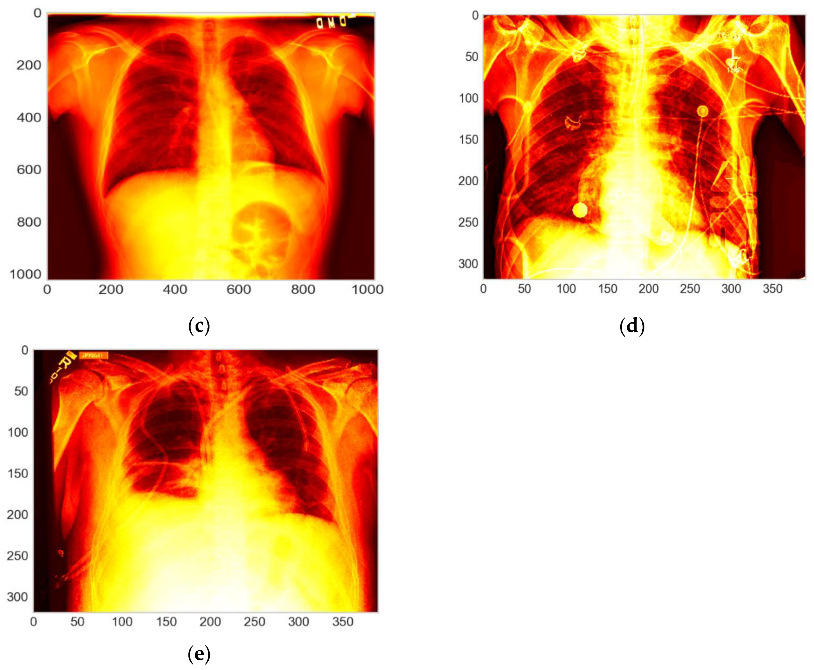
As one of the principal results of the EDA, we contemplated that the images of both datasets were from different dimensions, the images from [
20] were of 320 × 390 pixels in the height and the width, respectively. On the other hand, the images from [
21] were of 1028 × 1028 pixels in height and width. In addition, the images from both datasets were in the grayscale, which were homogenized. For this purpose, it is important to resize images to the same dimension, but to maintain a certain quality of the color scales (and allow greyscales to be comparable), the resizing needs to be in both cases a downscaling in order to obtain images with a similar quality for the two databases.
2.5. Image Preprocessing
For having a homogeneous dataset for the algorithm training, it is fundamental to homogenize/standardize the data. Therefore, we took the sample with 1086 images per category to work with a balance classification problem. We used a Holdout [
28] rate of 80%, 10%, and 10%, for the train, validation, and test sets, respectively. In addition, we used different techniques to prevent the overfitting as data augmentation [
29] and early stopping [
30]. Finally, we made an evaluation of the classification results on the test set by calculating the confusion matrix [
31] (p. 2), recall (True positive ratio, TPR) [
31] (p. 3), accuracy (ACC) [
31] (p. 3), precision (Positive Predictive Value, PPV) [
31] (p. 2) F1-score (F1) [
31] (p. 5), and the area under the receiver-operating characteristic curve (ROC AUC) [
32].
In this phase, first, we divided the sample into three groups, i.e., training, validation, and test sets, with the ratios of 80%, 10% and 10%, respectively, using the method in [
28]. Then, we applied a resizing of the height and width of each image to 150 × 150 pixels. Second, we used the method in [
29] for the training and validation sets. The transformations applied were the zoom-in, horizontal flip, rotation between 0 and 5 degrees, and normalization of each pixel of the different images, dividing every pixel of the images by 255.0 to achieve 0 as the minimum value and 1 as the maximum value (
Figure 3).
2.6. CNN Programming, Transfer Learning, and CNN Modifications
In this work, we used two CNNs. First, as the base model and feature extraction, we used the model in [
17]. Besides, we applied the transfer learning technique using the weights configuration from the ImageNet dataset [
33] and unfroze the weights for the last 2 convolutional blocks of [
17] on our dataset. The transfer learning technique consisted in using the weights of the CNN trained for a similar propose, i.e., classification problem, preconfigured in one dataset. In this case, we used the weights achieved in the Imagenet dataset [
33].
CNNs were adapted to image processing, being able to process two-dimensional (2D) or three-dimensional (3D) images. Here, we focused on 2D images. To do that, different types of layers were used, from which we included mainly two layers—convolutional (Conv) and pooling (Pool) layers. A convolutional layer is the core building element of a CNN, in which the features are detected, filtered and identified. A pooling layer (or downsampling layer) is used for dimensionality reduction, reducing the number of parameters in the input. A pooling minimization layer can also be used. The algorithm starts by processing the inputs with the first core convolutional layer, a succession of convolutional layers, and eventually pooling or min pooling layers plus a final synthesis layer. With each layer, the CNN increases the complexity to identify greater portions of the image. Earlier layers focus on simple features, such as colors and edges. As the image data progress through the various layers of the CNN algorithm, it is able to recognize larger elements or shapes of the X-ray image until it finally identifies the intended object and then assigns the image to a disease category. We started with a basic model [
17], which blocked the succession as illustrated in
Table 2.
We added three blocks composed by a convolutional layer [
34], a max pooling layer [
35] and a dropout layer [
36] to the base model. Finally, we added two dense blocks composed of a dense layer [
36], and a classification layer. As regularization related to the model architecture, we added a simple regularization procedure [
36] and L2 regularization [
37] to the kernel of the dense block. Finally, used the categorical cross-entropy loss [
38] as the loss function and Softmax [
39] as the activation function for the last classification layer. In other words, the proposed CNN works as follows:
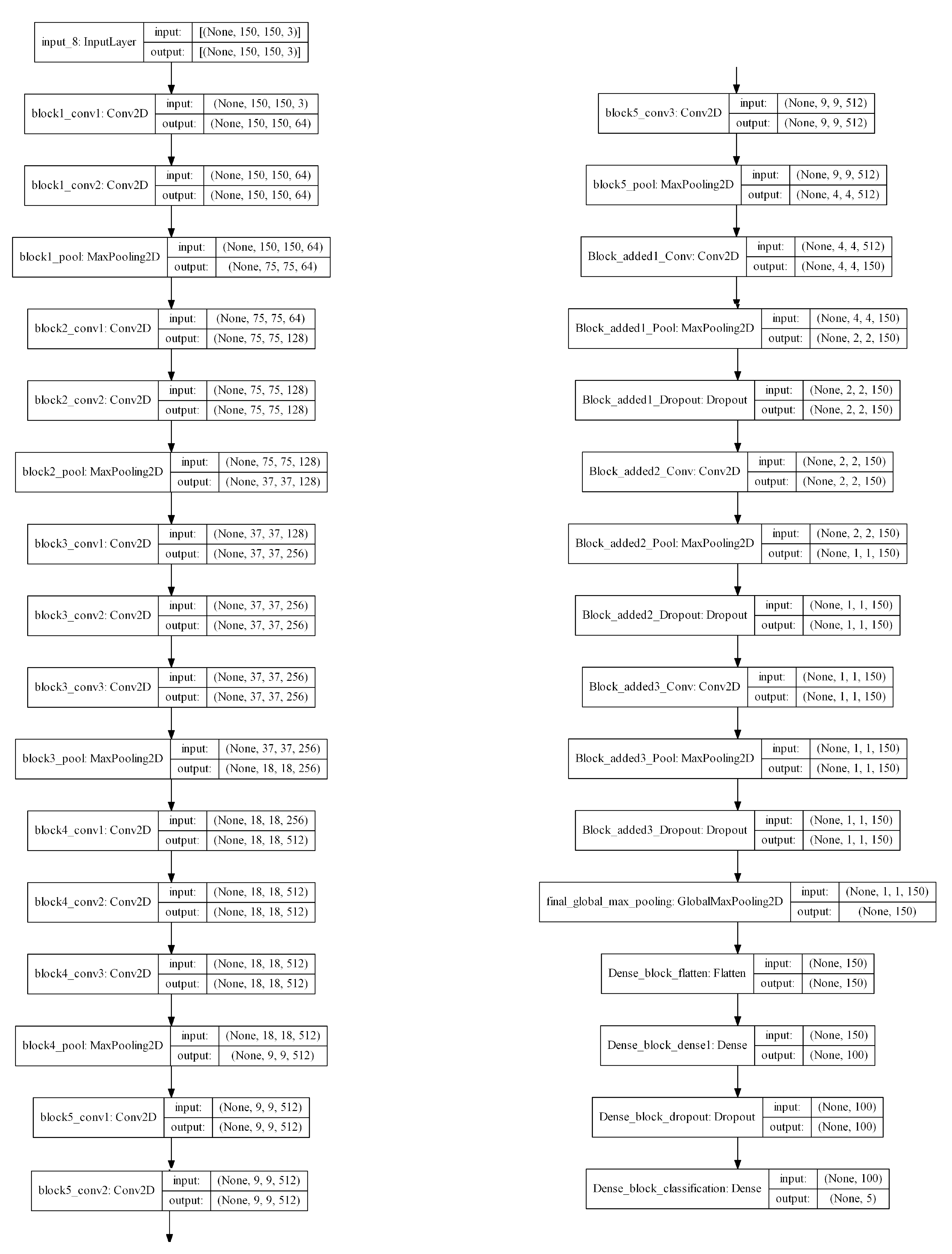
These convolutional blocks were composed of 2 or 3 convolutional layers using 128, 256, and 512 filters and 3 × 3 kernels. The convolutional blocks added to the base CNN were composed of a convolutional layer with 150 filters, 3 × 3 kernels, with the ReLU activation function, and a 2D max pooling layer. The dense block was composed of a dense layer using the ReLU as the activation function, 100 neurons, and the last classification layer with Softmax as the activation function and categorical cross-entropy as the loss function. The details of such blocks are in
Table 3 and the complete architecture is charted in the
Appendix A.
The final architecture of the algorithm, which shows how each block is combined, is given in the
Appendix A. The combination of the blocks is sequential.
2.7. CNN Training
We used a personal computer with Intel
® Core i7™—RAM 8GB and Nvidia
® Geforce GTX™ 1050. The operated system was Windows
® 10, professional edition. The dataset developed for the work was composed of 16,372 images where around 86% were from [
20] and about 14% were from [
21]. The images were classified in five different lung diseases, i.e., atelectasis, cardiomegaly, consolidation, edema, and pleural effusion (
Figure 4).
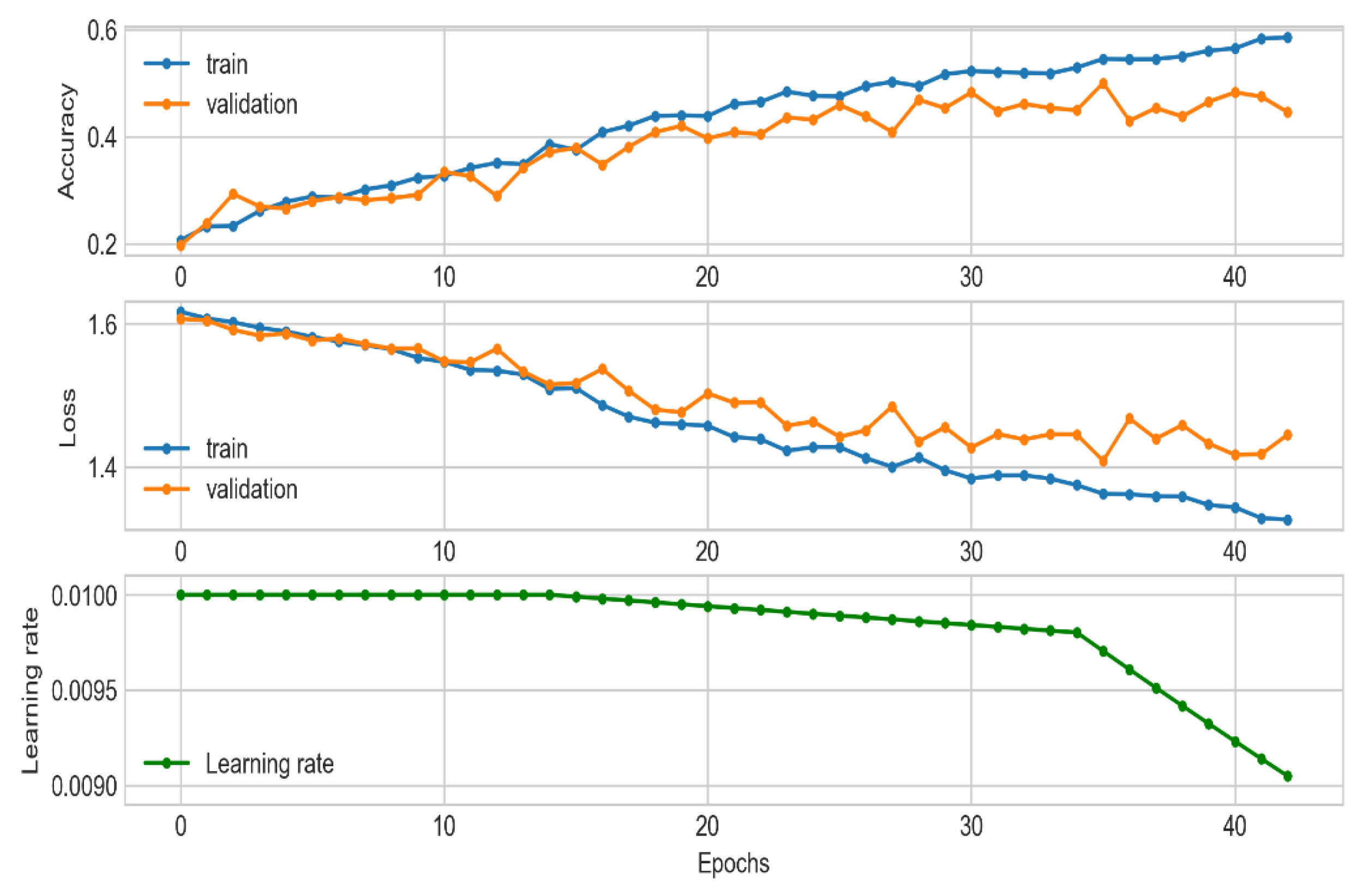
For the training process, we set up the training for 100 epochs, we used the adaptive moment estimation (Adam) [
40] optimizer with the configuration of
Table 1, an initial learning rate (LR) of 0.01, and a batch size of 128. To optimize this process and avoid the overfitting state of the CNN, we used early stopping [
30] to monitor the loss function on the validation set and the exponential decay [
41] of the LR scheduling and the model weights checkpoint (
Figure 5).
At the end of the training phase, we achieved an ACC of 50% at epoch 37, and the process stopped at epoch 44 due to [
30]. In addition, the LR decreased exponentially, and the minimum value achieved was 0.009048 at epoch 44 (
Table 4,
Figure 6).
3. Computational Results
For the testing set, we computed and plotted the confusion matrix [
31] (
Figure 5) and calculated the ACC, TPR, PPV, and F1. The results showed that, with the testing set, we achieved a general ACC about of 56%, which is a satisfactory result taking into account the literature and the use of affordable hardware. Besides, the TPRs were 31%, 23%, and 21% for atelectasis, consolidation, and cardiomegaly, respectively. On the other hand, we obtained F1-scores of 25%, 25%, 22%, and 21% for cardiomegaly, atelectasis, edema, and consolidation, respectively (
Table 5).
Those results are far from those obtained in the literature, but it is important to take into account the difference in the classification problem (here, we aimed to identify only one disease; in the literature works dealing with multiple diseases give a set of possible diseases for each image [
17,
18,
41]). For those reasons, it seems difficult to compare raw results (in terms of the TPR or the AUC, for example) between the proposed algorithm and the literature, since they do not address exactly the same problem. Moreover, when considering the false negative rate (FNR), defined as the ratio between the images not being assigned to any category (so considered as good health) and the total number of positives, we observed that for most pathologies the FNR was less than 1%, which is a good result (the cited works, by their nature and problem addressed, lead to the calculated FNRs of 1% to 3% [
18,
19]).
Taking into account those results and the fact that the hardware used is common and not of high performance, the results lead to a problem resolution issue that, for the medical field in Chile, seems satisfactory and represents the needs of the practice community. Only for one disease, i.e., pleural effusion, the algorithm seems to have a lower performance, but it is, if taking the FNR indicator (i.e., the risk of not diagnosing an illness of the patient when he or she has one), still good. In any case, the proposed algorithm is able to provide a support to medical decision making but needs to be seen as a complementary tool that do not have to substitute the choices of medical experts. Taking into account the quality of the computing infrastructures and the results of the model, its use is aimed to support medical decisions but does not identify clearly a disease in a way a human decision is not required: it must be then used as a support, but not as a substitute of the decision made.
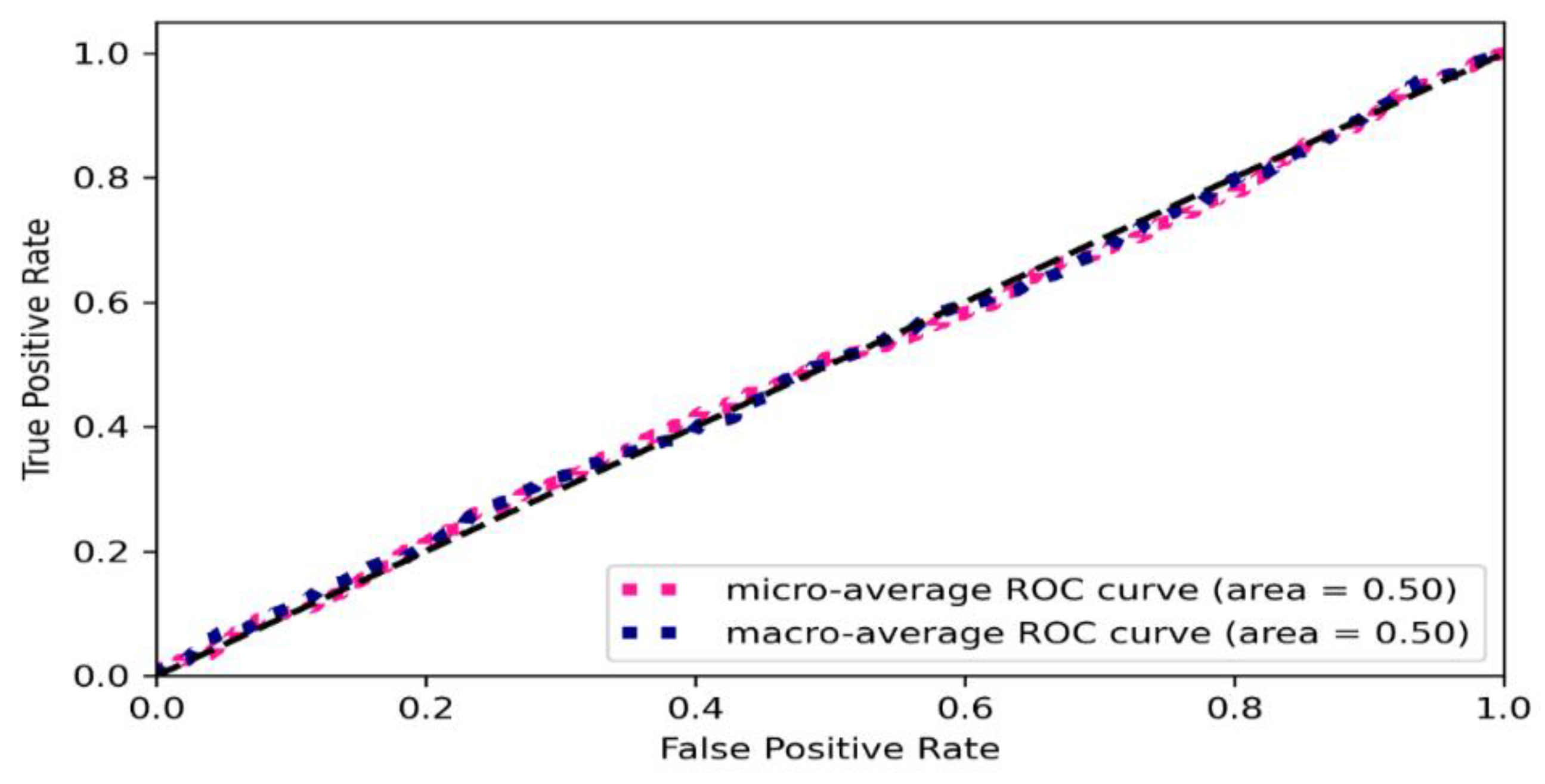
Figure 6 shows the ROC curve of the proposed algorithms. We carried out an ROC AUC analysis for the test set. We observed that the micro-average and macro-average ROCs are very close and both curves (ROC and AUC) are close and near linear, cutting the graph plane in two almost equal sets. We can then state that on the ROC AUC, the algorithm got about 50% (
Figure 6). When considering the identification on a unique disease for each image, it seems evident that if associating each image with more than one disease the quality of the model would increase, but in that case, the need of a medical staff decision is also observed. Therefore, using the proposed algorithm as a way to support medical decisions by informing the presence of a disease but need a specialist to define in-depth what the disease is seems to be suitable and recommended in contexts with resource constraints.
4. Conclusions
We trained a classifier of CXRs using different techniques. For the extraction of features, the VGG16 architecture was employed with their respective weights used in the ImageNet competition. The linear feature architecture was tuned; however, its linearity was maintained by adding new convolutional blocks and a dense block. In addition, different regularization techniques were employed, L2 was incorporated into the dense block, and dropout layers were added to all the blocks in the base architecture. Besides, in the training phase, we used data augmentation, scheduled a variable LR with an exponential decay, and early stopping to monitor the validation loss function.
The results obtained were not so good but are promising, because the training was not developed on extremely expensive hardware. However, this does not allow testing with batch sizes greater than 128. Of the PPV classification results, we achieved 30% with the cardiomegaly category. The highest TPR (31%) was achieved with the atelectasis category, and the highest F1 was achieved with the atelectasis and cardiomegaly categories, both of which were around 25%.
The proposed algorithm needs to be seen as a support for medical decision making. Indeed, it can help medical experts in having the first, graphical-statistical-based classification of X-ray images made on patients on the basis of a global database of diseases, which can help decide which disease the taken images represent. However, it does not have to be a substitute of medical expertise and human decisions but can be a valuable support, mainly in conditions where no high-quality hardware and material are available.
Finally, as a future work, we will replace the aggregated dropout layers with batch normalization layers, to analyze the training behavior of the network and the classification results. With better hardware, computational experiments with a larger batch size can be generated to improve the training results. The performance of federated learning for the training process will be evaluated.
Analyzing the performances of other nonlinear CNNs architectures such as DenseNet, MobileNet, ResNet, and Visual Transformers can be explored.
As for the data, the aim is to work together with a health institution to develop a representative dataset of our own, properly classified by a specialized medical team.
Author Contributions
Conceptualization, D.B. and G.G.; methodology, D.B., G.G. and J.G.-F.; validation, G.G. and J.G.-F.; formal analysis, D.B. and J.G.-F.; investigation, D.B. and G.G.; data curation, D.B.; writing—original draft preparation, D.B. and J.G.-F.; writing—review and editing, G.G.; project administration, G.G. All authors have read and agreed to the published version of the manuscript.
Funding
Part of this research was funded by a scholarship of the French Ambassy in Chile.
Institutional Review Board Statement
Not applicable.
Informed Consent Statement
Not applicable.
Data Availability Statement
Data employed to run the experiments are available from the corresponding references cited in the text.
Conflicts of Interest
The authors declare no conflict of interest. The funders had no role in the design of the study; in the collection, analyses, or interpretation of data; in the writing of the manuscript, or in the decision to publish the results.
Appendix A
Figure A1.
Architecture of the Convolutional Neural Networks algorithm with Transfer Learning.
Figure A1.
Architecture of the Convolutional Neural Networks algorithm with Transfer Learning.
References
- Le Cun, Y.; Boser, B.; Denker, J.; Henderson, D.; Howard, R.; Hubbard, W.; Jackel, L. Handwritten Digit Recognition with a Back-Propagation Network. In Advances in Neural Information Processing Systems; Morgan Kaufmann Publishers Inc.: San Francisco, CA, USA, 1989. [Google Scholar]
- Baccouche, A.; Garcia-Zapirain, B.; Olea, C.C.; Elmaghraby, A.S. Breast Lesions Detection and Classification via YOLO-Based Fusion Models. Comput. Mater. Contin. 2021, 69, 1407–1425. [Google Scholar] [CrossRef]
- Baumgartner, C.F.; Kamnitsas, K.; Matthew, J.; Smith, S.; Bernhard, K.; Rueckert, D. Real-Time Standard Scan Plane Detection and Localisation in Fetal Ultrasound Using Fully Convolutional Neural Networks. In Medical Image Computing and Computer-Assisted Intervention—MICCAI 2016, Proceedings of the 19th International Conference, Athens, Greece, 17–21 October 2016; Springer: Cham, Switzerland, 2016. [Google Scholar]
- Ronneberger, O.; Fischer, P.; Brox, T. U-Net: Convolutional Networks for Biomedical Image Segmentation. In Medical Image Computing and Computer-Assisted Intervention, Proceedings of the 18th International Conference, Munich, Germany, 5–9 October 2015; Springer: Cham, Switzerland, 2015. [Google Scholar]
- Çiçek, Ö.; Abdulkadir, A.; Lienkamp, S.S.; Brox, T.; Ronneberger, O. 3D U-Net: Learning Dense Volumetric Segmentation from Sparse Annotation. In Medical Image Computing and Computer-Assisted Intervention—MICCAI 2016, Proceedings of the 19th International Conference, Athens, Greece, 17–21 October 2016; Springer: Cham, Switzerland, 2016. [Google Scholar]
- Poudel, R.P.K.; Lamata, P.; Montana, G. Recurrent Fully Convolutional Neural Networks for Multi-slice MRI Cardiac Segmentation. In Medical Image Computing and Computer-Assisted Intervention—MICCAI 2016, Proceedings of the 19th International Conference, Athens, Greece, 17–21 October 2016; Springer: Cham, Switzerland, 2016. [Google Scholar]
- Anavi, Y.; Kogan, I.; Gelbart, E.; Geva, O.; Greenspan, H. A comparative study for chest radiograph image retrieval using binary texture and deep learning classification. In Proceedings of the 37th Annual International Conference of the IEEE Engineering in Medicine and Biology Society, Milan, Italy, 25–29 August 2015. [Google Scholar]
- Kim, E.; Corte-Real, M.; Baloch, Z. A deep semantic mobile application for thyroid cytopathology. In Proceedings of the Medical Imaging 2016: PACS and Imaging Informatics: Next Generation and Innovations, San Diego, CA, USA, 28–29 February 2016; Society of Photographic Instrumentation Engineers (SPIE): Bellingham, WA, USA, 2016; Volume 9789. [Google Scholar]
- Antony, J.; McGuinness, K.; O’Connor, N.E.; Moran, K. Quantifying Radiographic Knee Osteoarthritis Severity Using Deep Convolutional Neural Networks. 8 September 2016. Available online: https://arxiv.org/abs/1609.02469 (accessed on 24 November 2021).
- Ackoff, R.L. Optimization + objectivity = optout. Eur. J. Oper. Res. 1977, 1, 1–7. [Google Scholar] [CrossRef]
- Ruiz-Meza, J.; Meza-Peralta, K.; Montoya-Torres, J.R.; Gonzalez-Feliu, J. Location of Urban Logistics Spaces (ULS) for Two-Echelon Distribution Systems. Axioms 2021, 10, 214. [Google Scholar] [CrossRef]
- Szegedy, C.; Vanhoucke, V.; Ioffe, S.; Shlens, J.; Wojna, Z. Rethinking the Inception Architecture for Computer Vision. In Proceedings of the 2016 IEEE Conference on Computer Vision and Pattern Recognition (CVPR), Las Vegas, NV, USA, 27–30 June 2016. [Google Scholar]
- He, K.; Zhang, X.; Ren, S.; Sun, J. Deep Residual Learning for Image Recognition. In Proceedings of the IEEE Conference on Computer Vision and Pattern Recognition (CVPR), Las Vegas, NV, USA, 27–30 June 2016. [Google Scholar]
- Tan, M.; Le, Q.V. EfficientNet: Rethinking Model Scaling for Convolutional Neural Networks. In Proceedings of the International Conference on Machine Learning (ICML), Long Beach, CA, USA, 10–15 June 2019. [Google Scholar]
- Huang, G.; Liu, Z.; van der Maaten, L.; Weinberger, K.Q. Densely Connected Convolutional Networks. In Proceedings of the IEEE Conference on Computer Vision and Pattern Recognition (CVPR), Honolulu, HI, USA, 21–26 July 2017. [Google Scholar]
- Sandler, M.; Howard, A.; Zhu, M.; Zhmoginov, A.; Chen, L.-C. MobileNetV2: Inverted Residuals and Linear Bottlenecks. In Proceedings of the IEEE/CVF Conference on Computer Vision and Pattern Recognition, Salt Lake City, UT, USA, 18–23 June 2018. [Google Scholar]
- Simonyan, K.; Zisserman, A. Very Deep Convolutional Networks. In Proceedings of the International Conference on Learning Representations, San Diego, CA, USA, 7–9 May 2015. [Google Scholar]
- Liu, F.; Tang, J.; Ma, J.; Wang, C.; Ha, Q.; Yu, Y.; Zhou, Z. The application of artificial intelligence to chest medical image analysis. Intell. Med. 2021, 1, 104–117. [Google Scholar] [CrossRef]
- Subramanian, N.; Elharrouss, O.; Al-Maadeed, S.; Chowdhury, M. A review of deep learning-based detection methods for COVID-19. Comput. Biol. Med. 2022, 143, 105233. [Google Scholar] [CrossRef] [PubMed]
- Irvin, J.; Rajpurkar, P.; Ko, M.; Yu, Y.; Ciurea-Ilcus, S.; Chute, C.; Marklund, H.; Haghgoo, B.; Ball, R.; Shpanskaya, K.; et al. CheXpert: A Large Chest Radiograph Dataset with Uncertainty Labels and Expert Comparison. In Proceedings of the Thirty-Third AAAI Conference on Artificial Intelligence, Honolulu, HI, USA, 27 January–1 February 2019. [Google Scholar]
- Wang, C.; Yan, X.; Smith, M.; Kochhar, K.; Rubin, M.; Warren, S.M.; Wrobel, J.; Lee, H. A unified framework for automatic wound segmentation and analysis with deep convolutional neural networks. In Proceedings of the 37th Annual International Conference of the IEEE Engineering in Medicine and Biology Society (EMBC), Milan, Italy, 25–29 August 2015. [Google Scholar]
- Ackoff, R.L. A concept of corporate planning. Long Range Plan. 1970, 3, 2–8. [Google Scholar] [CrossRef]
- Ackoff, R.L. A Brief Guido to Interactive Planning and Idealized Design. 31 May 2021. Available online: https://www.ida.liu.se/~steho87/und/htdd01/AckoffGuidetoIdealizedRedesign.pdf (accessed on 25 November 2021).
- Gonzalez-Feliu, J. Logistics and Transport Modeling in Urban Goods Movement; IGI Global: Hershey, PA, USA, 2019; p. 29. [Google Scholar]
- Ackoff, R.L. Disciplines, the two cultures, and the scianities. Syst. Res. Behav. Sci. 1999, 16, 533–537. [Google Scholar] [CrossRef]
- Ackoff, R.L.; Pourdehnad, J. On misdirected systems. Syst. Res. Behav. Sci. 2001, 18, 199–205. [Google Scholar] [CrossRef]
- Ministerio de Salud de Chile (MINSAL). Guia de Practica Clinica Neumonia Adquirida en la Comunidad en Personas de 65 Añosy Mas. 1 December 2017. Available online: https://diprece.minsal.cl/le-informamos/auge/acceso-guias-clinicas/guias-clinicas-desarrolladas-utilizando-manual-metodologico/neumonia-adquirida-en-la-comunidad-de-manejo-ambulatorio-en-mayores-de-65-anos-y-mas/autores/ (accessed on 11 November 2021).
- Raschka, S. Model Evaluation, Model Selection, and Algorithm Selection in Machine Learning. 13 November 2018. Available online: https://arxiv.org/abs/1811.12808 (accessed on 11 January 2021).
- Abdollahi, B.; Tomita, N.; Hassanpour, S. Data Augmentation in Training Deep Learning Models for Medical Image Analysis. In Deep Learners and Deep Learner Descriptors for Medical Applications; Springer Nature: Cham, Switzerland, 2020; pp. 167–180. [Google Scholar]
- Prechelt, L. Early Stopping—But When. In Neural Networks: Tricks of the Trade; Springer: Berlin/Heidelberg, Germany, 2012; pp. 53–67. [Google Scholar]
- Grandini, M.; Bagli, E.; Visani, G. Metrics for Multi-Class Classification: An Overview. arXiv 2020, arXiv:2008.05756. [Google Scholar]
- Luque, A.; Carrasco, A.; Martin, A.; Lama, J.R. Exploring Symmetry of Binary Classification Performance Metrics. Symmetry 2019, 11, 47. [Google Scholar] [CrossRef] [Green Version]
- Russakovsky, O.; Deng, J.; Su, H.; Krause, J.; Satheesh, S.; Ma, S.; Huang, Z.; Karpathy, A.; Khosla, A.; Bernstein, M.; et al. ImageNet Large Scale Visual Recognition Challenge. Int. J. Comput. Vis. 2015, 115, 211–252. [Google Scholar] [CrossRef] [Green Version]
- Teuwen, J.; Moriakov, N. Convolutional Neural Networks. In Handbook of Medical Image Computing and Computer Assisted Intervention; Elsevier: Amsterdam, The Netherlands, 2020; pp. 481–501. [Google Scholar]
- Dominik, S.; Andreas, M.; Sven, B. Evaluation of Pooling Operations in Convolutional Architectures for Object Recognition. In Artificial Neural Networks—ICANN 2010, Proceedings of the 20th International Conference, Thessaloniki, Greece, 15–18 September 2010; Springer Nature: Cham, Switzerland, 2010. [Google Scholar]
- Srivastava, N.; Hinton, G.; Krizhevsky, A.; Sutskever, I.; Salakhutdinov, R. Dropout: A Simple Way to Prevent Neural Networks from Overfitting. J. Mach. Learn. 2014, 15, 1929–1958. [Google Scholar]
- Cortes, C.; Mohri, M.; Rostamizadeh, A. L2 Regularization for Learning Kernels. In Proceedings of the Twenty-Fifth Conference on Uncertainty in Artificial Intelligence, Montreal, QC, Canada, 18–21 June 2009. [Google Scholar]
- Geron, A. Hands on Machine Learning with Scikit-Learn, Keras and TensorFlow: Concepts, Tools, and Techniques to Biuld Intelligent Systems, 2nd ed.; O’reilly Media, Inc.: Sebastopol, CA, USA, 2019; p. 149. [Google Scholar]
- Nwankpa, C.; Ijomah, W.; Gachagan, A.; Marshall, S. Activation Functions: Comparison of trends in Practice and Research for Deep Learning. arXiv 2018, arXiv:1811.03378. [Google Scholar]
- Ruder, S. An Overview of Gradient Descent Optimization Algorithms. 15 September 2016. Available online: https://arxiv.org/abs/1609.04747 (accessed on 15 February 2022).
- Chougrad, H.; Zouaki, H.; Alheyane, O. Convolutional Neural Networks for Breast Cancer Screening: Transfer Learning with Exponential Decay. In Proceedings of the NIPS ML4H 2017: Machine Learning for Health Workshop at NIPS 2017, Long Beach, CA, USA, 8 December 2017. [Google Scholar]
| Publisher’s Note: MDPI stays neutral with regard to jurisdictional claims in published maps and institutional affiliations. |
© 2022 by the authors. Licensee MDPI, Basel, Switzerland. This article is an open access article distributed under the terms and conditions of the Creative Commons Attribution (CC BY) license (https://creativecommons.org/licenses/by/4.0/).


