Article

Modelling Coronavirus and Larvae Pyrausta Data: A Discrete Binomial Exponential II Distribution with Properties, Classical and Bayesian Estimation

by
Mohamed S. Eliwa
1,2,3,*,
Abhishek Tyagi
4,
Bader Almohaimeed
5 and
Mahmoud El-Morshedy
6,7
1
Department of Statistics and Operation Research, College of Science, Qassim University, Buraydah 51482, Saudi Arabia
2
Section of Mathematics, International Telematic University Uninettuno, I-00186 Rome, Italy
3
Department of Mathematics, Faculty of Science, Mansoura University, Mansoura 35516, Egypt
4
Department of Statistics, Chaudhary Charan Singh University, Ramgarhi, Meerut 250001, Uttar Pradesh, India
5
Department of Mathematics, College of Science, Qassim University, Buraydah 51482, Saudi Arabia
6
Department of Mathematics, College of Science and Humanities in Al-Kharj, Prince Sattam bin Abdulaziz University, Al-Kharj 11942, Saudi Arabia
7
Department of Statistics and Computer Science, Faculty of Science, Mansoura University, Mansoura 35516, Egypt
*
Author to whom correspondence should be addressed.
Axioms 2022, 11(11), 646; https://doi.org/10.3390/axioms11110646
Submission received: 14 October 2022 / Revised: 8 November 2022 / Accepted: 11 November 2022 / Published: 16 November 2022

Abstract

:
In this article, we propose the discrete version of the binomial exponential II distribution for modelling count data. Some of its statistical properties including hazard rate function, mode, moments, skewness, kurtosis, and index of dispersion are derived. The shape of the failure rate function is increasing. Moreover, the proposed model is appropriate for modelling equi-, over- and under-dispersed data. The parameter estimation through the classical point of view has been done using the method of maximum likelihood, whereas, in the Bayesian framework, assuming independent beta priors of model parameters, the Metropolis–Hastings algorithm within Gibbs sampler is used to obtain sample-based Bayes estimates of the unknown parameters of the proposed model. A detailed simulation study is carried out to examine the outcomes of maximum likelihood and Bayesian estimators. Finally, two distinctive real data sets are analyzed using the proposed model. These applications showed the flexibility of the new distribution.

1. Introduction

Fitting a probability distribution to real data and synthesizing information from it is a challenging task for statisticians/researchers. Data generated from day-to-day work environments are more complex in nature nowadays, and consequently several lifetime models have been proposed and studied in the literature to analyze these data. The well-known exponential distribution is one of the basic continuous models used to examine continuous data. However, Bakouch et al. [1] developed the binomial exponential II (BiExII) distribution, an extended variant of the ordinary exponential distribution, to provide additional flexibility. The BiExII model is constructed as a distribution of a random sum of independent exponential (Ex) random variables when the sample size has a zero-truncated binomial (Bi) distribution. The cumulative distribution function (CDF) of the BiExII model can be written as
G ( y ; λ , θ ) = 1 1 + λ θ y 2 θ e λ y ; y > 0 ,
where 0 θ 1 is the shape parameter and λ > 0 is the scale parameter. The probability density function (PDF) corresponding to Equation (1) can be expressed as
g ( y ; λ , θ ) = λ 1 + ( λ y 1 ) θ 2 θ e λ y ; y > 0 .
As we observe from Equation (1), the Ex distribution is a particular case for θ = 0 , whereas for θ = 1 , the gamma model with shape parameter 2 and scale parameter λ is a special case. Thus, Equation (2) can be written as
g ( y ; λ , θ ) = w λ e λ y + ( 1 w ) λ 2 y e λ y ; y > 0 ,
where w = 2 ( 1 θ ) 2 θ . Habibi and Asgharzadeh [2] presented a power binomial exponential distribution by applying the power transformation on BiExII random variable. The hazard rate function of the proposed distribution portrays the decreasing, increasing, decreasing-increasing-decreasing and unimodal shapes. Al-babtain et al. [3] developed a new extension of the BiExII model using the Marshall–Olkin (MO-G) family of distributions. They have also discussed a simple type Copula-based construction to derive the bivariate- and multivariate-type distributions. Recently, Zhang et al. [4] first reviewed the two-parameter Poisson binomial-exponential 2 (PBE2) distribution, then they proposed a new integer-valued auto-regressive (INAR) model with PBE2 innovations.
Sometimes reliability/survival experiments yield data which are discrete in nature either due to limitations of measuring instruments or its inherent characteristic. For example, in reliability engineering, the number of successful cycle prior to the failure when device work in cycle, the number of times a device is switched on/off; in survival analysis, the survival times for those suffering from the diseases such as lung cancer or period from remission to relapse may be recorded as number of days/weeks, number of deaths/daily cases due to COVID-19 pandemic observed over a specified duration, etc. Moreover, in many practical problems, the count phenomenon occurs as, for example, the number of occurrences of earthquakes in a calendar year, the number of absences, the number of accidents, the number of kinds of species in ecology, the number of insurance claims, and so on. Therefore, it is reasonable to model such situations by a suitable discrete distribution.
Discretization of continuous models can be done by utilizing various techniques. The most widely used approach is the survival discretization method. One of the important virtues of this methodology is that the developed discrete distribution retains the same functional form of the survival function as that of its continuous counterpart. Due to this feature many reliability characteristics of the distribution remain unchanged. According to this method, for a given continuous random variable (RV) Y with survival function (SF) S Y ( y ) = P ( Y y ) , the RV X = [ Y ] (largest integer less than or equal to Y) will have the probability mass function
P ( X = x ) = S Y ( x ) S Y ( x + 1 ) ; x = 0 , 1 , 2 , 3 . . . .
Many authors have used Equation (4) for generating the discrete analogue of the continuous distributions, for instance, discrete Rayleigh distribution (Roy [5]), discrete Burr and Pareto distributions (Krishna and Pundir [6]), discrete gamma distribution (Chakraborty and Chakravarty [7]), discrete modified Weibull distribution (Almalki and Nadarajah [8]), discrete generalized exponential and exponentiated discrete Weibull distributions (Nekoukhou and Bidram [9,10]), discrete extended Weibull distribution (Jia et al. [11]), geometric-zero truncated Poisson distribution (Akdogan et al. [12]), Poisson quasi-Lindley regression model and Poisson–Bilal distribution (Altun [13,14]), discrete Burr–Hatke distribution (El-Morshedy et al. [15]), discrete inverted Nadarajah–Haghighi distributions (Singh et al. [16]), discrete Teissier distribution (Singh et al. [17]), and related references cited therein.
In view of the existing literature, we found that several discrete distributions have been introduced over the past few decades. Yet there is much scope left to introduce new plausible discrete distributions that can adequately capture the diversity of real data. This phenomenon motivates us to provide a flexible discrete model for fitting a wide spectrum of discrete real-world data sets. Therefore, in this paper, we have proposed the discrete analogue of the BiExII model, in the so-called discrete BiExII (DBiExII) distribution using survival discretization method. An important motivation of the proposed study is that the BiExII distribution has manageable and closed-form expressions for various important distributional properties, including probability mass function, cumulative distribution function, moments, etc. Furthermore, discrete data generated from many practical studies, such as mortality experiments, industrial experiments, etc., show constant or increasing failure rates, so the proposed distribution is useful for modelling monotonically increasing failure rate data. Other motivations for developing the BiExII distribution include its ability to analyze not only equi-, over-, and under-dispersed real data, but also a positively skewed, or leptokurtic data set. A final motivation for the new distribution is that the proposed distribution is capable of modelling count data as we will see later, and by this, it provides a well alternative to several discrete distributions for modelling discrete data in applications.
The rest of the article is organized as follows. In Section 2, we have introduced the DBiExII model. Different distributional characteristics are discussed in Section 3. In 
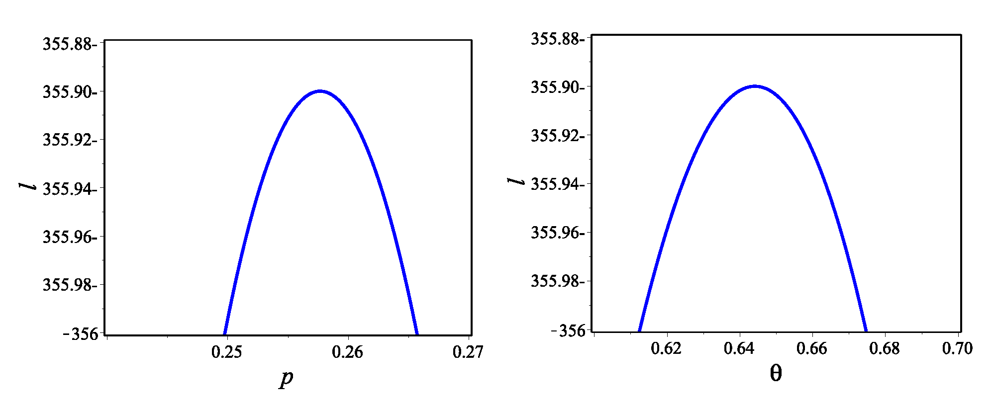
Section 4, the model parameters are estimated by using maximum likelihood and Bayesian methods. Simulation study is presented in 
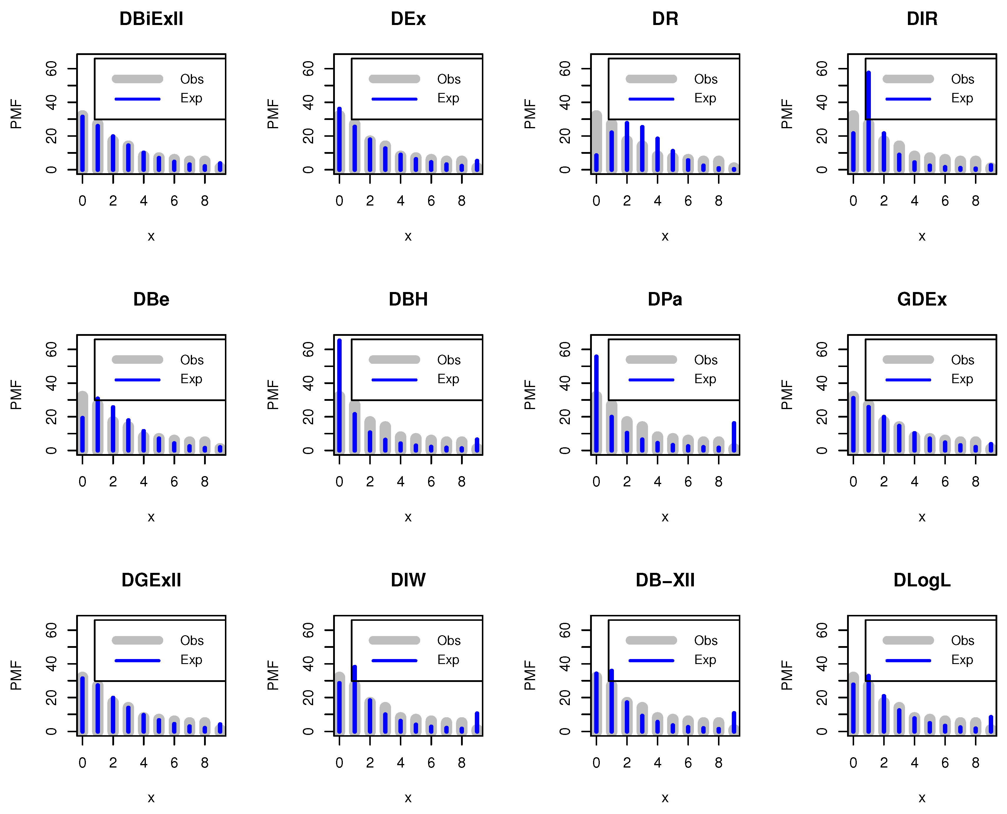
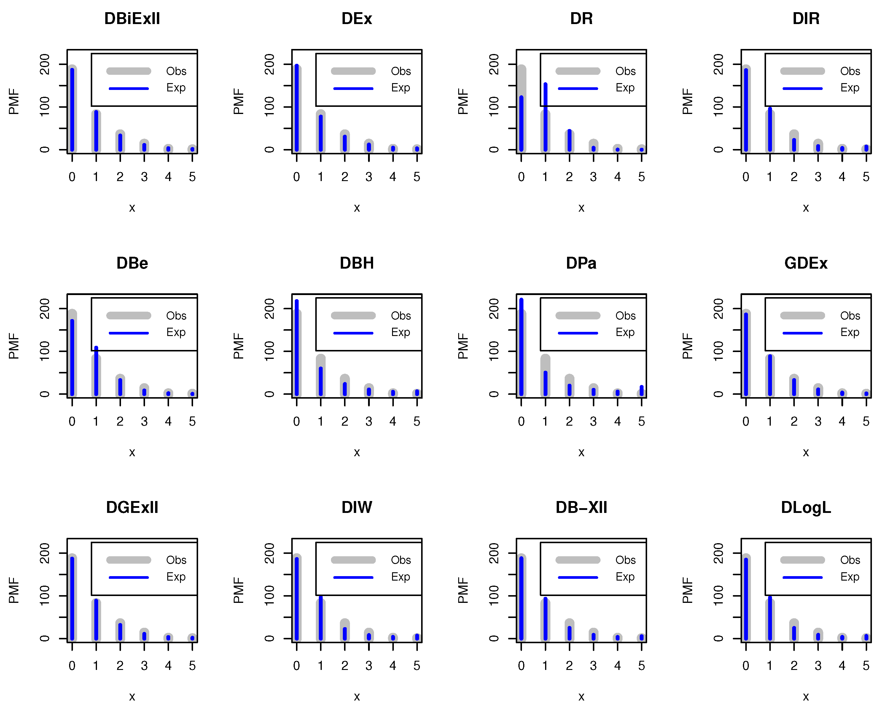
Section 5. The two real data sets (COVID-19 and larvae Pyrausta) are analyzed to show the flexibility of the DBiExII distribution in Section 6. Finally, Section 7 provides some conclusions.

2. The DBiExII Distribution

Using the Equation (4), the probability mass function (PMF) of the DBiExII distribution with positive parameters 0 < p < 1 and 0 θ 1 , can be derived as
f ( x ; p , θ ) = 1 p + θ ( p x + p x ) ln p 2 θ p x ; x N 0 ,
where p = e λ and N 0 = 0 , 1 , 2 , 3 , . . . . The cumulative distribution function (CDF) corresponding to Equation (5) can be expressed as
F ( x ; p , θ ) = f ( X x ; p , θ ) = i = 0 x f ( i ; p , θ ) = 1 1 θ ( x + 1 ) ln p 2 θ p x + 1 ; x N 0 .
The behavior of the CDF of the DBiExII distribution can be described as
F ( x ; p , θ ) = p θ ( ln p + 1 ) + 2 p + θ 2 θ 2 ; x 0 , 1 p x + 1 ; θ 0 , p x + 1 ( x ln p + ln p 1 ) + 1 ; θ 1 .
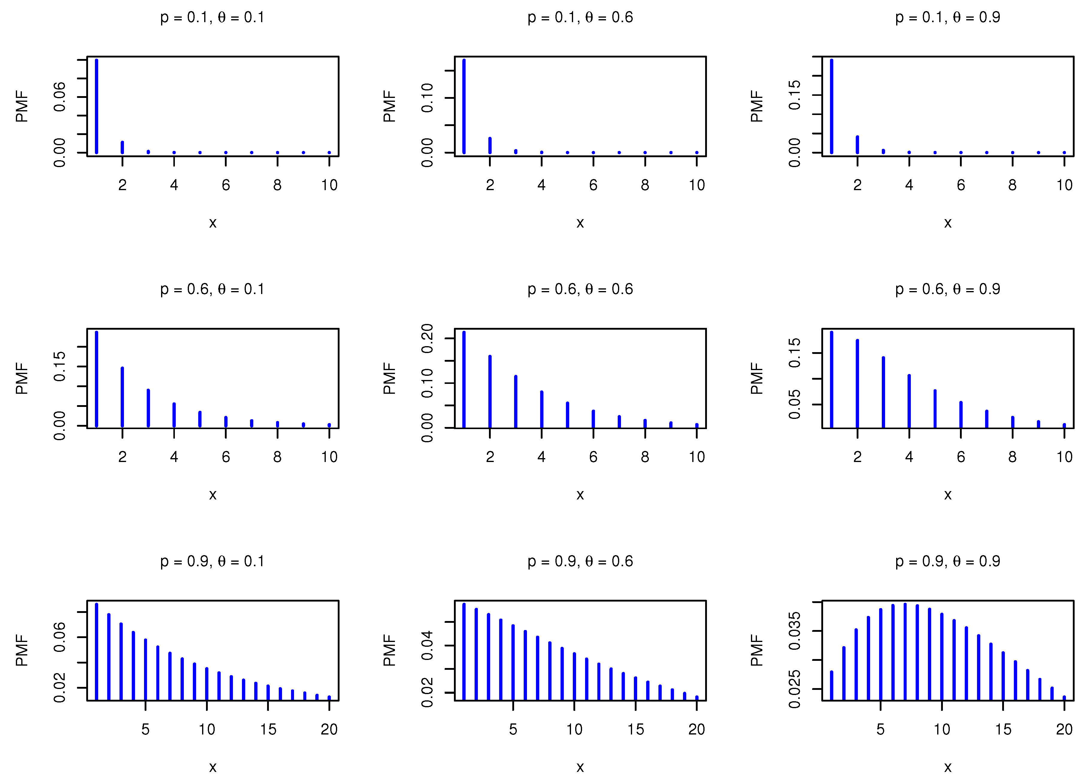
The behavior of the PMF is given by
f ( x ; p , θ ) = p θ ( ln p + 1 ) + 2 p + θ 2 θ 2 ; x 0 , p x ( 1 p ) ; θ 0 , p x [ ( p x + p x ) ln p p + 1 ] ; θ 1 .
The PMF in Equation (5) is log-concave, where f ( x + 1 ; p , θ ) f ( x ; p , θ ) is a decreasing function in x for all values of the model parameters, and consequently the PMF is unimodal and right-skewed. Figure 1 shows the PMF plots for different values of the parameters.
The PMF can take unimodal or decreasing-shaped. Assume X has a DBiExII distribution with parameters p and θ . Then, the PMFs of Z = X 2 and U = X + a can be formulated, respectively, as
f z ( z ; p , θ ) = 1 2 z 1 p + θ ( p z + p z ) ln p 2 θ p z ; z { 0 , 1 , 4 , 9 , 16 , . . . }
and
f u ( u ; p , θ ) = 1 p + θ ( p ( u a ) + p u + a ) ln p 2 θ p u a ; u { a , a + 1 , a + 2 , . . . } ,
where 
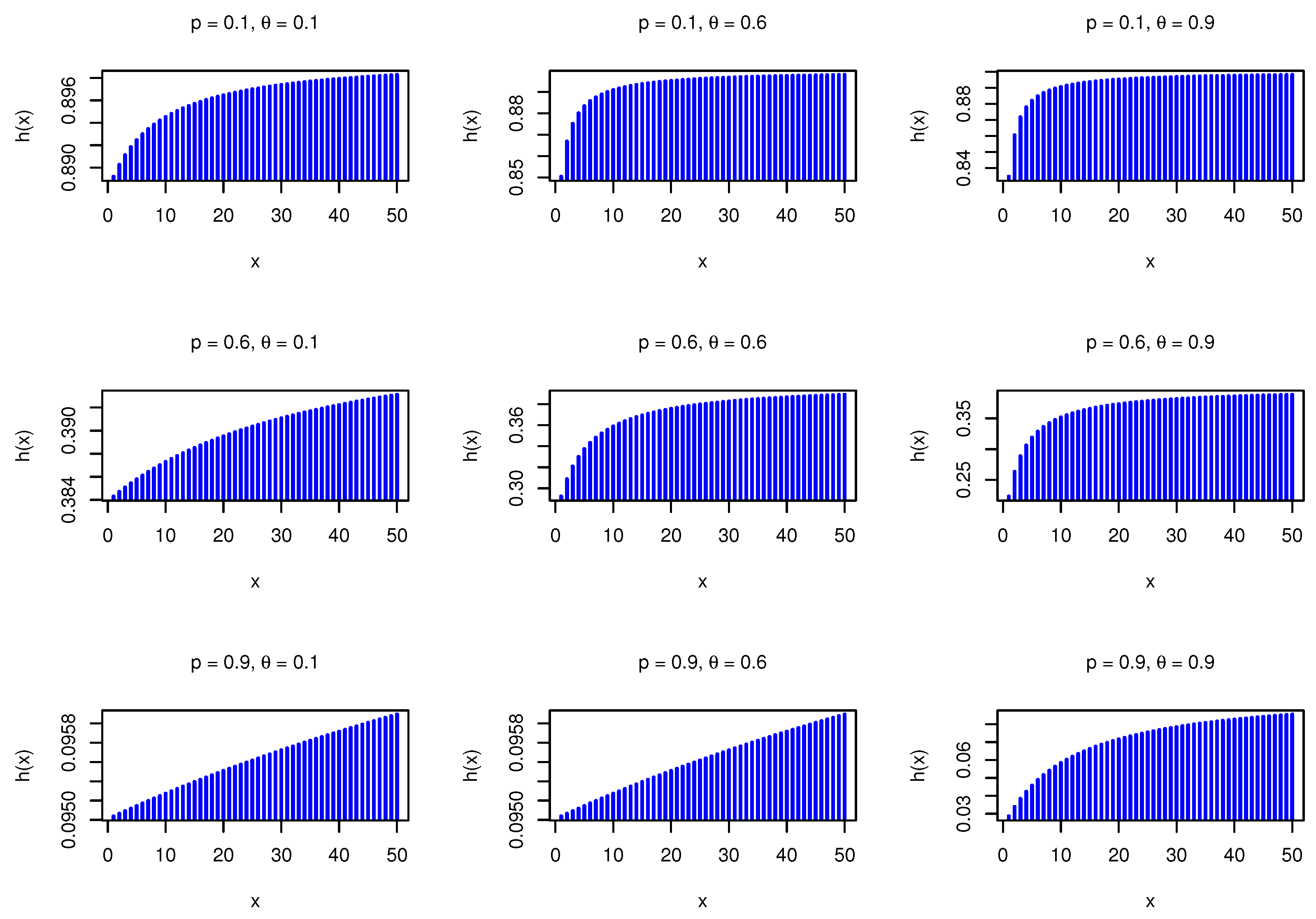
a is a positive integer number. The hazard rate function (HRF) of the DBiExII model can be expressed as
h ( x ; p , θ ) = ( 2 θ ) ( 1 p ) + θ ( p x + p x ) ln p 2 θ ( 1 + x ln p ) ; x N 0 ,
where h ( x ; p , θ ) = f ( x ; p , θ ) 1 F ( x 1 ; p , θ ) . The behavior of the HRF is given by
h ( x ; p , θ ) = p θ ( 1 + ln p ) + 2 p + θ 2 θ 2 ; x 0 , 1 p ; x , 1 p ; θ 0 , ( p x + p x ) ln p + p 1 x ln p 1 ; θ 1 .
Based on the log-concavity properties, the DBiExII distribution has increasing failure rate. For more details around the log-concave function (Gupta and Balakrishnan [18]). Figure 2 shows the HRF plots for different values of the parameters.
It is observed that the HRF takes increasing shape. The second rate of failure (SRF) is given by
h * ( x ; p , θ ) = log θ x ln p + θ 2 p [ θ x ln p + θ ln p + θ 2 ] ,
where h * ( x ; p , θ ) = log 1 F ( x 1 ; p , θ ) 1 F ( x ; p , θ ) . The behavior of the SRF is given by
h * ( x ; p , θ ) = log θ 2 p [ θ ln p + θ 2 ] ; x 0 , ln 1 p ; x , ln 1 p ; θ 0 , log x ln p 1 p [ x ln p + ln p 1 ] ; θ 1 .
For more details about the difference between the HRF and SRF, we can refer to (Xie et al. [19]).

3. Distributional Statistics

3.1. Mode

If X has a DBiExII model, then the mode can be obtained by solving the following non-linear equation
1 p ( 2 θ ) + θ ( p x + p x ) ln p p x ln p + θ ( p 1 ) p x ln p = 0 .
Then, the mode of the DBiExII model is given by
M ( X ) = θ p ( ln p + 2 ) 2 ( p + θ 2 ) θ ( p 1 ) ln p .

3.2. Moments, Skewness, Kurtosis and Index of Dispersion

Suppose the RV X follows DBiExII distribution. Then, the probability generating function (PGF) can be formulated in an explicit form as
Π X ( t ; p , θ ) = p θ ( t 1 ) ln p + ( p 1 ) ( p t 1 ) ( θ 2 ) ( p t 1 ) 2 ( θ 2 ) ,
where Π X ( t ; p , θ ) = x = 0 t x f ( x ; p , θ ) . On Replacing t by e t in Equation (17), we get the moment generating function (MGF). Thus, the MGF can be proposed as
Π X * ( t ; p , θ ) = p θ ( e t 1 ) ln p + ( p 1 ) ( p e t 1 ) ( θ 2 ) ( p e t 1 ) 2 ( θ 2 ) .
The first four derivatives of the MGF, with respect to t at t = 0 , yield the first four moments about the origin. So, the first four moments of the DBiExII model are
E ( X ) = p θ ln p + ( p 1 ) ( θ 2 ) ( p 1 ) 2 ( θ 2 ) ,
E ( X 2 ) = p ( 3 p 1 ) θ ln p + p 2 θ 2 p 2 θ + 2 ( p 1 ) 3 ( θ 2 ) ,
E ( X 3 ) = p ( 7 p 2 θ 10 p θ θ ) ln p + ( θ 2 ) ( p 1 ) ( p 2 + 4 p + 1 ) ( p 1 ) 4 ( θ 2 )
and
E ( X 4 ) = p 150 ( p 3 + 11 3 p 2 + 5 3 p + 1 15 ) ln p + ( p 2 + 10 p + 1 ) ( p 2 1 ) ( θ 2 ) ( p 1 ) 5 ( θ 2 ) .
The variance of the DBiExII model can be calculated by using Var ( X ) = E ( X 2 ) E ( X ) 2 . Using well-known relations, it is also simple to compute the skewness and kurtosis measures of the DBiExII model. The shape characteristics for both mean and variance of the DBiExII distribution can be formulated, respectively, as
E ( X ) = p 1 p ; θ 0 , p ( ln p p + 1 ) p 2 2 p + 1 ; θ 1
and
Variance ( X ) = p p 2 2 p + 1 ; θ 0 , ( p 3 p 2 ln p p ) ln p + p 3 2 p 2 + p p 4 4 p 3 + 6 p 2 4 p + 1 ; θ 1 ,
The index of dispersion (IxD, for short) is defined as variance to mean ratio, it indicates whether a certain model is suitable for under or over-dispersed data sets. If IxD < ( > 1 ) , the model is under- (over-) dispersed. If X has a DBiExII model, then the behavior of the IxD is given by
IxD = 1 1 p ; θ 0 , ( p ln p p 2 + 1 ) ln p p 2 + 2 p 1 ( p 2 2 p + 1 ) ln p + p 3 3 p 2 + 3 p 1 ; θ 1 ,
In order to provide a numerical illustration of the pattern of the moments and associated features, we have calculated these properties for a variety of values of the parameters, and the results can be found in Table 1.
From Table 1, it is clear that the DBiExII distribution is appropriate for modelling under-, equi-, and over-dispersed data sets. Moreover, the proposed model can be used for modelling positively skewed and leptokurtic data sets.

4. Parameter Estimation

Here, we discuss the point and interval estimation of the unknown parameters of DBiExII distribution using classical and Bayesian estimation.

4.1. Point Estimation through Maximum Likelihood Approach

In this section, we determine the maximum likelihood estimates (MLEs) of the model parameters based on complete sample. Let X 1 , X 2 , X n be a random sample of size n from the DBiExII model. Then, the likelihood function (L) is given by
L ( x ̲ ; p , θ ) = p i = 1 n x i i = 1 n 1 p + θ ( p x i + p x i ) ln p 2 θ ,
and the respective log-likelihood function (l) is
l ( x ̲ ; p , θ ) = ln ( p ) i = 1 n x i + i = 1 n ln 1 p + θ p x i + 1 x i ln ( p ) 2 θ .
By differentiating Equation (27) with respect to the parameters p and θ , respectively, we get the non-linear likelihood equations as follows
1 p ^ i = 1 n x i + i = 1 n θ ^ 2 + θ ^ x i + 1 ln ( p ^ ) + x i + 1 x i p ^ ( 1 p ^ ) ( 2 θ ^ ) + θ ^ p ^ x i + 1 x i ln ( p ^ ) = 0
and
i = 1 n 2 p ^ x i + 1 x i ln ( p ^ ) ( 2 θ ^ ) ( 1 p ^ ) ( 2 θ ^ ) + θ ^ p ^ x i + 1 x i ln ( p ^ ) = 0 .
Equations (28) and (29) cannot be solved analytically; therefore, the suggested system needs an iterative procedure such as Newton-Raphson to solve these two equations numerically.

4.2. Asymptotic Confidence Interval

Unfortunately, the MLE of the unknown parameter vector Λ = ( p , θ ) T has no closed-form expression, so it is not possible to develop the exact confidence interval (CIs) for the parameter vector Λ . Hence, we derived the asymptotic confidence interval (ACI) for Λ by utilizing its asymptotic distribution. For this purpose, let Λ ^ = ( p ^ , θ ^ ) T be the estimate of Λ = ( p , θ ) T and the parameter vector Λ has the following Fisher’s information matrix,
I ( Λ ) = E 2 l p 2 2 l p θ 2 l θ p 2 l θ 2 .
Thus, under some regularity conditions with large n, n ( Λ ^ Λ ) follows bivariate normal distribution with zero mean vector and variance-covariance matrix as I 1 ( Λ ) . Here, I 1 ( Λ ) is the inverse of the expected Fisher’s information matrix I ( Λ ) . Due to the complexity of the PMF of the random variable X, the expected values in I ( Λ ) is not easily obtainable, therefore we utilized the estimated observed Fisher’s information matrix that can be symbolized as
I ( Λ ^ ) 2 l p 2 ( p ^ , θ ^ ) 2 l p θ ( p ^ , θ ^ ) 2 l θ p ( p ^ , θ ^ ) 2 l θ 2 ( p ^ , θ ^ ) ,
where, p ^ and θ ^ are the MLEs of p and θ , respectively. The expressions for second order partial derivatives used in above observed Fisher’s information matrix are as follows
2 l p 2 = 1 p 2 i = 1 n x i + i = 1 n θ [ ( 1 p ) ( 2 θ ) + θ [ p ( x i + 1 ) x i ] ln ( p ) ] x i + 1 p + x i p ( 2 θ ) θ ( x i + 1 ) ( 1 + ln ( p ) ) ( x i / p ) 2 [ ( 1 p ) ( 2 θ ) + θ [ p ( x i + 1 ) x i ] ln ( p ) ] 2 ,
2 l θ 2 = 4 i = 1 n [ p ( x i + 1 ) x i ] ln ( p ) ( 1 p ) ( 2 θ ) ( 1 θ ) [ p ( x i + 1 ) x i ] ln ( p ) ( 2 θ ) [ ( 1 p ) ( 2 θ ) + θ [ p ( x i + 1 ) x i ] ln ( p ) ] 2 ,
and
2 l p θ = 2 i = 1 n ( 1 p ) [ p ( x i + 1 ) x i ] ( 1 p ) [ p ( x i + 1 ) x i ] p p + ln ( p ) [ ( 1 p ) ( 2 θ ) + θ [ p ( x i + 1 ) x i ] ln ( p ) ] 2 .
Hence, ( 1 γ ) × 100 % ACI for parameters Λ i ; i = 1 , 2 is given by
Λ ^ i Z 1 γ / 2 V a r ( Λ ^ i ) , Λ ^ i Z 1 γ / 2 V a r ( Λ ^ i ) ; i = 1 , 2 ,
where V a r ( Λ ^ i ) is the ( i , i ) t h diagonal element of I 1 ( Λ ) and Z 1 γ / 2 is the ( 1 γ / 2 ) t h quantile of the standard normal distribution.

4.3. Bayesian Estimation

Over the past few decades, the importance of Bayesian statistics has increased immensely, not only because Bayesian estimators have become much easier to calculate, but also because it is one of the most satisfactory ways of calculating estimates for complex models. In this context, the present section is devoted to the Bayesian estimation of the unknown parameters of DBiExII distribution. Let the prior beliefs regarding the unknown parameters, p and θ are represented through the independent priors as beta distribution of first kind with respective densities as
π 1 ( p ) p a 1 1 ( 1 p ) b 1 1 , 0 < p < 1 ,
π 2 ( θ ) θ a 2 1 ( 1 θ ) b 2 1 , 0 < θ < 1 ,
where the shape parameters a 1 , b 1 , a 2 and b 2 are known and non-negative. These parameters are also named as hyper parameters which can be adjusted to indicate the prior information about the unknown parameters of the model. The joint prior distribution of p and θ is
π 12 ( p , θ ) p a 1 1 ( 1 p ) b 1 1 θ a 2 1 ( 1 θ ) b 2 1 , 0 < p < 1 , 0 < θ < 1 .
Combining the likelihood function in Equation (26) and the joint prior distribution in Equation (32) using Bayes’ theorem, the joint posterior distribution of p and θ given data is derived as
π 0 ( p , θ | x ̲ ) p i = 1 n x i + a 1 1 ( 1 p ) b 1 1 θ a 2 1 ( 1 θ ) b 2 1 i = 1 n 1 p + θ ( p x + p x ) ln ( p ) 2 θ .
In theBayesian scenario, a correct statistical decision depends not only on the choice of prior distribution, but it also relies on the selection of appropriate loss function. Therefore, to draw Bayesian inferences on unknown parameters p and θ , we should take care of the question of which type of loss function will be used. Here, we use the most common symmetric loss function, which is as popular as the squared error loss function (SELF). It is symmetric in the sense that it equally penalizes overestimation and underestimation. If κ ^ is an estimator of κ , then we can define the SELF as
L o s s ( κ ^ , κ ) = ( κ ^ κ ) 2 .
Thus, in our case, the Bayes estimator (BE) of any function of parameters p and θ , say ϕ ( p , θ ) under SELF with informative priors (IPs) is obtained as
ϕ ^ ( p , θ | x ̲ ) = E p , θ | x ̲ ( ϕ ( p , θ ) ) = 0 1 0 1 ϕ ( p , θ ) π 0 ( p , θ | x ̲ ) d p d θ .
Here, it can be easily observed that the integral in Equation (35) cannot solved analytically, this is because of the complex form of joint posterior distribution in Equation (33). Therefore, we use popular Markov Chain Monte Carlo (MCMC) technique known as Gibbs sampler (Geman and Geman [20]). The biggest virtue of this algorithm is that it allows us to generate posterior samples for all the parameters using their full conditional posterior distribution. In this context, the full conditional posterior distributions of the parameters p and θ can be written as
W ( p | θ , x ̲ ) p i = 1 n x i + a 1 1 ( 1 p ) b 1 1 i = 1 n 1 p + θ ( p x + p x ) ln ( p ) 2 θ
and
V ( θ | p , x ̲ ) θ a 2 1 ( 1 θ ) b 2 1 i = 1 n 1 p + θ ( p x + p x ) ln ( p ) 2 θ .
Here, it is notable that the generation of parameters draws on p and θ from their respective posterior densities (36) and (37) are not possible through conventional methods of generating samples, therefore we used the Metropolis–Hastings (MH) algorithm advocated by (Devroye [21]). We utilized the following steps of Gibbs sampling algorithm:
  • Plug in with the initial values of p and θ , as ( p ( 0 ) , θ ( 0 ) ) .
  • Start with j = 1 .
  • Generate p ( j ) from the conditional posterior distribution in Equation (36), through MH algorithm with normal proposal distribution.
  • Generate θ ( j ) from the conditional posterior density in Equation (37) using MH algorithm with normal proposal distribution.
  • Set j = j + 1 .
  • Repeat the steps 3–5, a large number of times, say N times, and obtain p ( j ) and θ ( j ) , j = 1 , 2 , 3 , , N .
To ensure convergence and avoid the effect of selecting initial values, the first M draws are eliminated. Then, the remaining values p ( j ) and θ ( j ) , j = M + 1 , M + 2 , , N , represent the required posterior samples, which can be utilized to draw the Bayesian conclusions about the unknown population constraints. Hence, the Bayes estimates of p and θ under SELF, respectively, obtained as
p ^ B E = 1 N M j = M + 1 N p ( j ) and θ ^ B E = 1 N M j = M + 1 N θ ( j ) .
If a prior distribution provides limited or no information about the parameter, it is called a non-informative prior (NIP). The reasoning for utilizing NIPs is often said to be ‘to let the data speak for themselves,’ so that posterior inferences are ineffective by information external to the sample data. However, finding a suitable prior distribution for a parameter is a daunting task. Although there is a vast literature on how to select an appropriate prior for a parameter of interest (Berger [22]; Bernado and Smith [23]), the choice of priors remains a challenging issue. Various NIPs are available in the existing literature, but uniform (or flat) prior are widely applied in practice. As suggested by an honourable reviewer, here, we use non-informative uniform priors for p and θ and they can be obtained by putting a 1 = b 1 = a 2 = b 2 = 1 in Equations (30) and (31). Hence, proceeding similarly as we do in the case of IPs, we can obtain the Bayes estimators with SELF under NIPs.

4.4. Highest Posterior Density (HPD) Credible Interval

A Bayesian counterpart of the classical confidence interval is called a credible or probability interval and it can be explained in a probabilistic manner. This differs from a traditional confidence interval, which can only be expressed in terms of coverage probability. We can easily obtain an equal-tail credible interval ( α L , α U ) for a parameter α by simplifying the following equations:
0 α L π ( α | x ̲ ) d α = γ 2 and 0 α U π ( α | x ̲ ) d α = 1 γ 2 ,
where π ( α | x ̲ ) denotes the posterior distribution of the unknown parameter α and γ represents the level of significance. We can construct several such credible intervals, but to derive the best among them, we select the interval with the smallest width. The shortest interval, let us say ( α L h , α U h ) , is the credible interval that fulfills the following two conditions:
( i ) . α L h α U h π ( α | x ̲ ) d α = 1 γ . ( i i ) . For any α 1 ( α L h , α U h ) and α 2 ( α L h , α U h ) we have π ( α 1 | x ̲ ) > π ( α 2 | x ̲ ) .
This type of credible interval is called the highest posterior density (HPD) credible interval. Since, the mathematical derivation of the HPD credible intervals for the unknown parameters of DBiExII distribution is difficult to obtain due to the non-closure form of the posterior distributions, therefore, we use an algorithm suggested by Chen and Shao [24]. For this purpose, consider the MCMC samples, p ( j ) and θ ( j ) , j = M + 1 , M + 2 , , N , generated in the previous section. Now, ordered these generated values as p ( M + 1 ) < p ( M + 2 ) < . . . < p ( N ) and θ ( M + 1 ) < θ ( M + 2 ) < . . . < θ ( N ) . Thus, the ( 1 γ ) × 100 % HPD credible intervals for p and θ are respectively given as
p ( M + j * ) , p ( M + j * + [ ( 1 γ ) ( N M ) ] ) and ( θ ( M + j * * ) , θ ( M + j * * + [ ( 1 γ ) ( N M ) ] ) ) ,
where j * and j * * are respectively chosen so that
p ( M + j * + [ ( 1 γ ) ( N M ) ] ) p ( M + j * ) = min M j ( N M ) [ ( 1 γ ) ( N M ) ] p ( M + j + [ ( 1 γ ) ( N M ) ] ) p ( M + j )
and
θ ( M + j * * + [ ( 1 γ ) ( N M ) ] ) θ ( M + j * * ) = min M j ( N M ) [ ( 1 γ ) ( N M ) ] θ ( M + j + [ ( 1 γ ) ( N M ) ] ) θ ( M + j ) .

5. Numerical Illustration through Simulated Data

In this section, we conduct a Monte Carlo simulation analysis to evaluate the behavior of classical and Bayesian procedures for estimating the unknown parameters of the DBiExII distribution. This study consists of the following steps:
Step 1.
Generate 10,000 samples of size n {20, 40, 60, 100} from DBiExII distribution using Equation (6) with the arbitrary sets of parameters ( p , θ ) {(0.3, 0.3), (0.3, 0.8), (0.8, 0.3), (0.5, 0.5), (0.8, 0.8)}.
Step 2.
Compute the MLEs, Bayes estimates (with NIPs and IPs), 95% asymptotic and HPD confidence intervals for each of the 10,000 samples.
In the case of Bayesian estimation, it is important to note that we have calculated the Bayes estimates with IPs and NIPs under SELF. In IPs, the prior densities for the parameters p and θ are taken to be B e t a 1 ( a 1 , b 1 ) and B e t a 1 ( a 2 , b 2 ) distributions, respectively. The hyper-parameters in these prior densities have been selected in such a manner that the mean of a parameter’s prior density is almost equal to the corresponding assumed value of that parameter, whereas, all hyper-parameters are set to 1 for Bayes estimation under NIPs. Using the algorithm described in Section 4.3, we produced 21,000 realizations of the Markov chain of p and θ from their full conditional posterior distributions in order to calculate the required Bayesian quantities. To counteract the impact of the parameters beginning values, the first 1000 burn-in values for each chain have been eliminated. Additionally, we have stored every tenth observation to reduce the autocorrelation between draws. By plotting MCMC runs, posterior densities, and the autocorrelation function for each pair of true parameters, the convergence of the produced chains is investigated. For the sake of simplicity, we have only included these graphs for ( p , θ ) = (0.3, 0.3) in Figure 3. After the convergence testing, we have utilized simulated posterior samples to compute Bayes estimates and HPD intervals.
Step 3.
Compute the average estimate (AE), root mean squared error (RMSE), and average absolute bias (AB) for MLEs and Bayes estimates (with SELF under IPs and NIPs), whereas for 95% asymptotic and HPD confidence intervals, we calculate average lower confidence limit (ALCL), average upper confidence limit (AUCL), average width (AW), and coverage probability (CP).
All the calculations have been done with R software. The outcomes of the simulation study are given in Table 2, Table 3, Table 4, Table 5, Table 6 and Table 7. From these tables, the following important conclusions can be drawn:
i.
The RMSE of both estimators decreases with increasing sample size. This validates the consistency property of the estimators. Moreover, as the value of n increases, the absolute bias decreases toward zero.
ii.
Bayes estimators obtained under IPs show smaller RMSE as compared to the MLEs and Bayes estimators with NIPs.
iii.
Under NIPs, the Bayesian method becomes the first choice of estimation in the absence of prior information. This is due to the fact that the Bayes estimates under NIPs have the smallest estimation errors when compared to the MLEs.
iv.
The average width of classical and Bayesian intervals becomes smaller as the sample size increases. Moreover, the HPD interval with IPs outperforms asymptotic and HPD intervals under NIPs in terms of the width of the intervals. The CPs are close to the corresponding nominal levels in both classical and Bayesian intervals.
v.
In both estimation processes, the estimation of θ is more sensitive than the estimation of p since it results in more estimation error relative to the other parameter.

6. Data Analysis

In this section, we illustrate the flexibility of the DBiExII distribution for modelling various types of data sets generated from different fields. We have compared the fits of the DBiExII model with some well-known existing models having one or two parameters and these are reported in Table 8. The fitted models are compared using famous criteria, namely, l (Negative log-likelihood), Akaike information criterion (AIC) “ A I C = 2 c 2 L ”, with its corrected value (CAIC) “ C A I C = [ 2 n c / ( n c 1 ) ] 2 L ”, and Chi-square ( χ 2 ) statistic with associated P-value, where L is the maximized likelihood function evaluated at MLEs, n is the sample size, and c is the number of parameters in the model.

6.1. Data Set I: COVID-19

The data are reported in (https://www.worldometers.info/coronavirus/country/south-korea/, 5 February to 13 June 2022) and represents the daily new deaths in South Korea country. The MLEs with their corresponding standard errors (Std-er), confidence interval (C. I) for the parameter(s) and goodness of fit statistic for data set I are listed in Table 9, Table 10 and Table 11.
From Table 10 and Table 11, the DBiExII model is the best distribution among all tested models. Figure 4 shows the profile of the log-likelihood function for data set I and this figure announces that the parameters are unimodal functions.
Figure 5 shows the estimated PMFs for data set I.
Table 12 lists some information about data set I based on the DBiExII model.
From Table 12, the empirical mean, variance, IxD are close to theoretical ones. Data set I suffers from overdispersion phenomena, and most of the distribution is at the left with leptokurtic character.

6.2. Data Set II: Larvae Pyrausta

This data set is the biological experiment data which represents the number of European corn borer larvae Pyrausta in field (Holt et al. [32]). The MLEs with their corresponding Std-ers, confidence intervals (C. Is) for the parameter(s) and goodness of fit statistic for data set II are listed in Table 13, Table 14 and Table 15.
From Table 14 and Table 15, the DBiExII distribution is the best model among all tested models. Figure 6 shows the profile of the log-likelihood function for data set II, and from this figure, it is clear that the parameters are unimodal functions.
Figure 7 shows the estimated PMFs for data set II.
Table 16 lists some information around data set II under the DBiExII model.
From Table 16, the theoretical mean, variance, IxD and skewness are close to empirical ones. Data set II suffers from overdispersion phenomena, and most of the distribution is at the left with leptokurtic character.

6.3. Bayesian Estimation for Data Sets I and II

In this sub-section, we calculate Bayes estimates and HPD credible intervals for the unknown parameters of DBiExII distribution under the real data set I and II. Due to the lack of prior information on these parameters for the given data sets, we assume the uniform NIPs for the unknown parameters of the model. Doing the same as we did in the simulation study in Section 5, we have computed the Bayes estimates with their associated posterior standard errors (PStd-ers) and HPD credible intervals for the unknown parameters p and θ under the data sets I and II. The resulted values are tabulated in Table 17.
For both data sets, when we have compared the Bayes estimates with the results of MLEs, we found that both methods work well, but Bayesian estimation with NIPs is superior than method of maximum likelihood in terms of estimation errors and length of the confidence intervals.

7. Conclusions

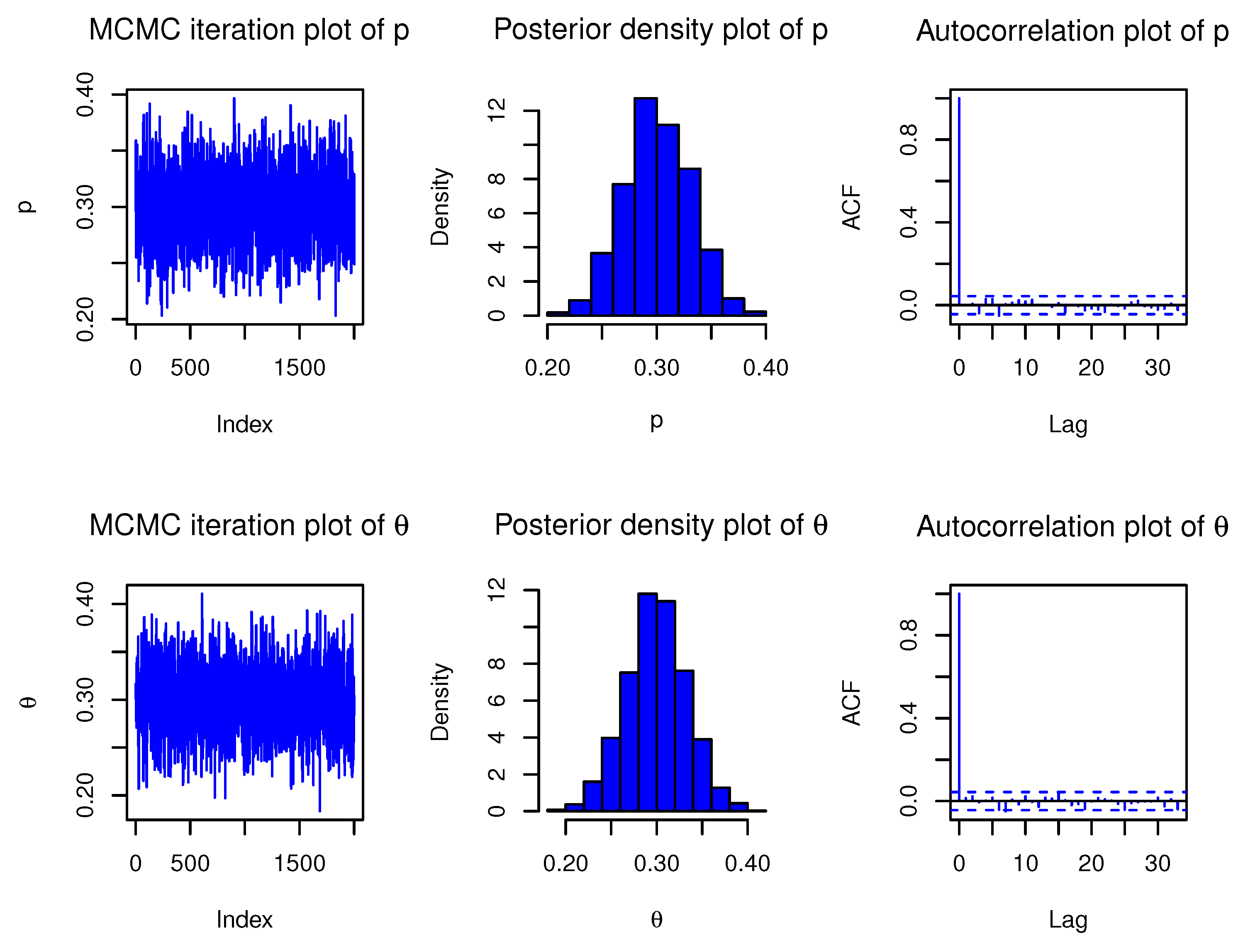
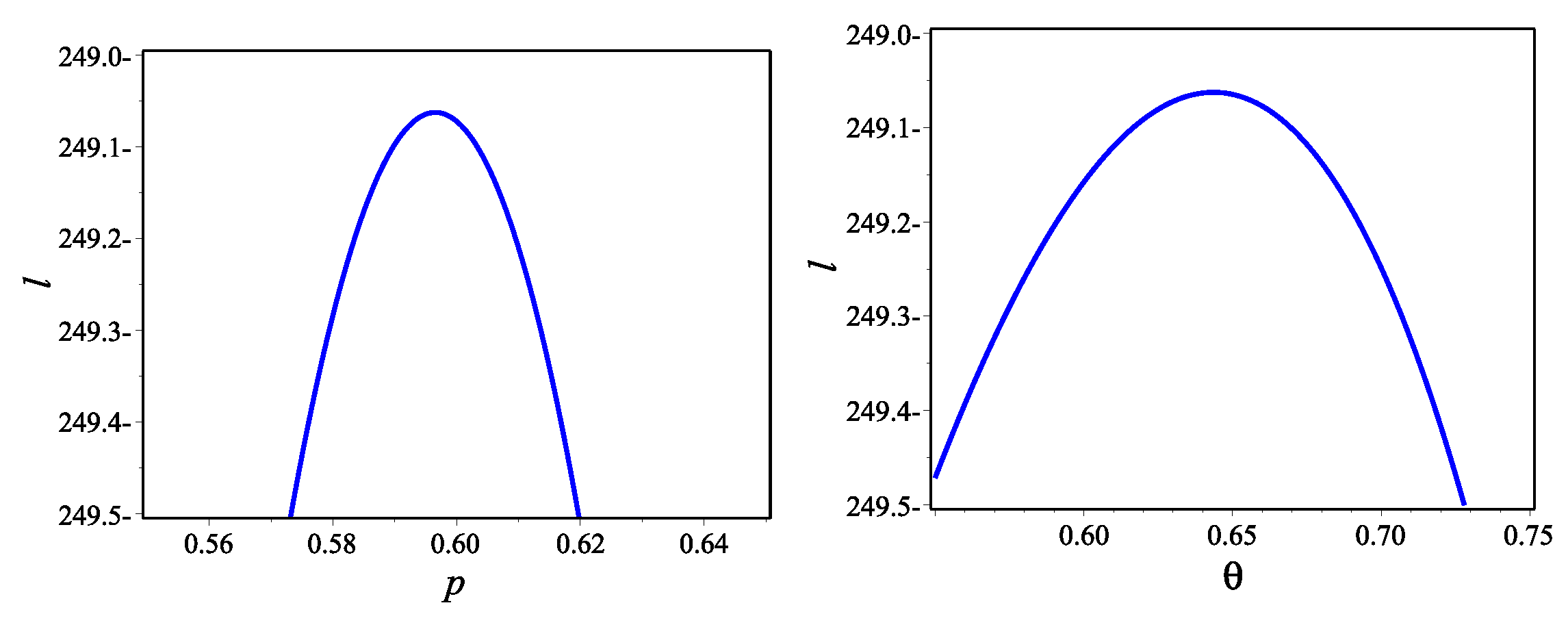
The present article introduced a new two-parameter discrete model, called discrete binomial exponential II distribution. We have discussed several important properties of the proposed model. One of the key advantages of this newly developed model is that it can model a variety of data (over-, equi-, and under-dispersed, positively skewed, leptokurtic, and increasing failure time data). Two well-known estimation techniques, the method of maximum likelihood and Bayesian estimation, have been used to derive the point and interval estimators of the unknown parameters of the DBiExII distribution.
A detailed Monte Carlo simulation study has been performed to test the behaviour of different point and interval estimators with respect to sample size and parametric values. The results of this numerical study show that both estimation methods work satisfactorily, but Bayesian estimation under beta priors dominates the method of maximum likelihood in terms of estimation errors. In the end, the usefulness of the new distribution is illustrated by means of two real data sets to prove its versatility in practical applications. We, therefore, believe that the DBiExII distribution may be a better alternative to some popular existing discrete models and may be widely applicable for modelling real-life data sets in various fields. With regard to future work, the researchers may use the new model to propose a bi-variate distribution based on the shock model approach for modelling bi-variate data. In addition, a regression model and a first-order integer-valued auto-regressive process can be studied in detail.

Author Contributions

Conceptualization, M.S.E. and A.T.; methodology, M.S.E. and B.A.; software, M.E.-M. and A.T.; validation, B.A., M.E.-M., and M.S.E.; formal analysis, M.S.E.; investigation, M.E.-M. and B.A.; data curation, M.E.-M. and A.T.; writing—original draft preparation, M.S.E. and M.E.-M.; writing—review and editing, M.S.E. and A.T.; visualization, M.E.-M. and B.A.; supervision, M.S.E. and M.E.-M.; project administration, M.S.E.; funding acquisition, M.S.E. and B.A. All authors have read and agreed to the published version of the manuscript.

Funding

Deputyship for Research & Innovation, Ministry of Education, Qassim University, Saudi Arabia under project number: QU-IF-2-2-4-25117.

Data Availability Statement

The data sets are available in the paper.

Acknowledgments

The authors extend their appreciation to the Deputyship for Research & Innovation, Ministry of Education, Saudi Arabia for funding this research work through the project number (QU-IF-2-2-4-25117). The authors also thank to Qassim University for technical support.

Conflicts of Interest

The authors declare no conflict of interest.

References

  1. Bakouch, H.S.; Jazi, M.A.; Nadarajah, S.; Dolati, A.; Roozegar, R. A lifetime model with increasing failure rate. Appl. Math. Model. 2014, 38, 5392–5406. [Google Scholar] [CrossRef]
  2. Habibi, M.; Asgharzadeh, A. Power binomial exponential distribution: Modelling, simulation and application. Commun. Stat.-Simul. Comput. 2018, 47, 3042–3061. [Google Scholar] [CrossRef]
  3. Al-babtain, A.A.; Elbatal, I.; Yousof, H.M. A new flexible three-parameter model: Properties, clayton copula, and modelling real data. Symmetry 2020, 12, 440. [Google Scholar] [CrossRef] [Green Version]
  4. Zhang, J.; Zhu, F.; Khan, N.M. A new INAR model based on Poisson-BE2 innovations. Commun. Stat.-Theory Methods 2021, 52, 1–15. [Google Scholar] [CrossRef]
  5. Roy, D. Discrete rayleigh distribution. IEEE Trans. Reliab. 2004, 53, 255–260. [Google Scholar] [CrossRef]
  6. Krishna, H.; Pundir, P.S. Discrete Burr and discrete Pareto distributions. Stat. Methodol. 2009, 6, 177–188. [Google Scholar] [CrossRef]
  7. Chakraborty, S.; Chakravarty, D. Discrete gamma distributions: Properties and parameter estimations. Commun. Stat.-Theory Methods 2012, 41, 3301–3324. [Google Scholar] [CrossRef]
  8. Almalki, S.J.; Nadarajah, S. A new discrete modified Weibull distribution. IEEE Trans. Reliab. 2014, 63, 68–80. [Google Scholar] [CrossRef]
  9. Nekoukhou, V.; Bidram, H. The exponentiated discrete Weibull distribution. Sort 2015, 39, 127–146. [Google Scholar]
  10. Nekoukhou, V.; Hamid, B. A new discrete distribution based on geometric odds ratio. J. Stat. Model. Theory Appl. 2020, 1, 153–166. [Google Scholar]
  11. Jia, J.M.; Yan, Z.Z.; Peng, X.Y. A new discrete extended Weibull distribution. IEEE Access 2019, 7, 175474–175486. [Google Scholar] [CrossRef]
  12. Akdogan, Y.; Coskun, K.U.S.; Bidram, H.; Kinaci, İ. Geometric-Zero Truncated Poisson Distribution: Properties and Applications. Gazi Univ. J. Sci. 2019, 32, 1339–1354. [Google Scholar] [CrossRef]
  13. Altun, E. A new model for over-dispersed count data: Poisson quasi-Lindley regression model. Math. Sci. 2019, 13, 241–247. [Google Scholar] [CrossRef] [Green Version]
  14. Altun, E. A new one-parameter discrete distribution with associated regression and integer-valued autoregressive models. Math. Slovaca 2020, 70, 979–994. [Google Scholar] [CrossRef]
  15. El-Morshedy, M.; Eliwa, M.S.; Altun, E. Discrete Burr-Hatke distribution with properties, estimation methods and regression model. IEEE Access 2020, 8, 74359–74370. [Google Scholar] [CrossRef]
  16. Singh, B.; Singh, R.P.; Nayal, A.S.; Tyagi, A. Discrete Inverted Nadarajah-Haghighi Distribution: Properties and Classical Estimation with Application to Complete and Censored data. Stat. Optim. Inf. Comput. 2022, 10, 1293–1313. [Google Scholar]
  17. Singh, B.; Agiwal, V.; Nayal, A.S.; Tyagi, A. A Discrete Analogue of Teissier Distribution: Properties and Classical Estimation with Application to Count Data. Reliab. Theory Appl. 2022, 17, 340–355. [Google Scholar]
  18. Gupta, R.C.; Balakrishnan, N. Log-concavity and monotonicity of hazard and reversed hazard functions of univariate and multivariate skew-normal distributions. Metrika 2012, 75, 181–191. [Google Scholar] [CrossRef]
  19. Xie, M.; Gaudoin, O.; Bracquemond, C. Redefining failure rate function for discrete distributions. Int. J. Reliab. Qual. Saf. Eng. 2002, 9, 275–285. [Google Scholar] [CrossRef]
  20. Geman, S.; Geman, D. Stochastic relaxation, Gibbs distributions, and the Bayesian restoration of images. IEEE Trans. OnPattern Anal. Mach. Intell. 1984, 6, 721–741. [Google Scholar] [CrossRef]
  21. Devroye, L. On the use of probability inequalities in random variate generation. J. Stat. Comput. Simul. 1984, 20, 91–100. [Google Scholar] [CrossRef]
  22. Berger, J.O. Prior information and subjective probability. In Statistical Decision Theory and Bayesian Analysis; Springer: New York, NY, USA, 1985; pp. 74–117. [Google Scholar]
  23. Bernado, J.M.; Smith, A.F.M. Bayesian Theory; Wiley: New York, NY, USA, 2000. [Google Scholar]
  24. Chen, M.H.; Shao, Q.M. Monte Carlo estimation of Bayesian credible and HPD intervals. J. Comput. Graph. 1999, 8, 69–92. [Google Scholar]
  25. Gómez-Déniz, E. Another generalization of the geometric distribution. Test 2010, 19, 399–415. [Google Scholar] [CrossRef]
  26. Nekoukhou, V.; Alamatsaz, M.H.; Bidram, H. Discrete generalized exponential distribution of a second type. Statistics 2013, 47, 876–887. [Google Scholar] [CrossRef]
  27. Hussain, T.; Ahmad, M. Discrete inverse Rayleigh distribution. Pak. J. Stat. 2014, 30, 15–32. [Google Scholar]
  28. Eliwa, M.S.; El-Morshedy, M.; Altun, E. A study on discrete Bilal distribution with properties and applications on integer-valued autoregressive process. Revstat-Stat. J. Forthcom. 2020, 20, 501–528. [Google Scholar]
  29. Jazi, A.M.; Lai, D.C.; Alamatsaz, H.M. Inverse Weibull distribution and estimation of its parameters. Stat. Methodol. 2010, 7, 121–132. [Google Scholar] [CrossRef]
  30. Para, B.A.; Jan, T.R. On discrete three parameter Burr type XII and discrete Lomax distributions and their applications to model count data from medical science. Biom. Biostat. J. 2016, 4, 1–15. [Google Scholar]
  31. Para, B.A.; Jan, T.R. Discrete version of log-logistic distribution and its applications in genetics. Int. Math. Math. Sci. 2016, 14, 407–422. [Google Scholar]
  32. Holt, A.R.; Gaston, K.J.; He, F. Occupancy-abundance relationships and spatial distribution: A review. Basic Appl. Ecol. 2002, 3, 1–13. [Google Scholar] [CrossRef]
Figure 1. The PMF for the DBiExII model.
Axioms 11 00646 g001
Figure 2. The HRF for the DBiExII model.
Axioms 11 00646 g002
Figure 3. MCMC diagnostics plots for DBiExII(0.3,0.3) distribution.
Axioms 11 00646 g003
Figure 4. The profile of l function for the model parameters based on data set I.
Axioms 11 00646 g004
Figure 5. The estimated PMFs for data set I.
Axioms 11 00646 g005
Figure 6. The profile of l function for the model parameters based on data set II.
Axioms 11 00646 g006
Figure 7. The estimated PMFs for data set II.
Axioms 11 00646 g007
Table 1. Some descriptive statistics for the DBiExII distribution.
ParameterMeasure
p θ MeanVarianceSkewnessKurtosisIxD
0.01 0.01 0.010337 0.010443 9.987279 104.743575 1.010326
0.1 0.012573 0.012719 9.072254 87.147341 1.011601
0.3 0.018392 0.018593 7.493631 60.338393 1.010916
0.5 0.025763 0.025936 6.293304 43.140116 1.006720
0.7 0.035401 0.035374 5.310417 31.192865 0.999238
0.9 0.048544 0.047945 4.457520 22.420924 0.987655
0.99 0.056157 0.055068 4.100374 19.193921 0.980612
0.1 0.01 0.112539 0.125201 3.462044 16.984848 1.112503
0.1 0.126072 0.141519 3.308182 15.870692 1.122521
0.3 0.161276 0.182253 2.946320 13.237950 1.130068
0.5 0.205867 0.230291 2.575399 10.759760 1.118638
0.7 0.264179 0.287110 2.201012 8.584148 1.086800
0.9 0.343695 0.353631 1.819239 6.743941 1.028908
0.99 0.3897517 0.386376 0.386376 6.031577 0.991341
0.3 0.01 0.432275 0.619110 2.369474 10.613745 1.432212
0.1 0.467367 0.682789 2.322009 10.336483 1.460926
0.3 0.558652 0.836902 2.161759 9.330162 1.498074
0.5 0.674280 1.008188 1.954587 8.141058 1.495206
0.7 0.825485 1.191830 1.721058 7.001209 1.443793
0.9 1.031674 1.368560 1.478955 6.065819 1.326542
0.99 1.151101 1.432036 1.376903 5.765703 1.244058
0.5 0.01 1.006966 2.020850 2.119947 9.493563 2.006869
0.1 1.072962 2.213565 2.095548 9.340058 2.063039
0.3 1.244640 2.674071 1.982932 8.611448 2.148469
0.5 1.462098 3.172759 1.819516 7.675631 2.170004
0.7 1.746466 3.682186 1.630544 6.767094 2.108364
0.9 2.134240 4.116220 1.447103 6.071141 1.928658
0.99 2.358842 4.230074 1.386767 5.901186 1.793283
0.9 0.01 9.047650 90.90308 2.002601 9.009693 10.04714
0.1 9.499076 99.23336 1.988878 8.906269 10.44663
0.3 10.67337 118.9939 1.899065 8.295979 11.14866
0.5 12.16081 140.0647 1.757718 7.474355 11.51770
0.7 14.10593 160.9421 1.592996 6.674835 11.40953
0.9 16.75836 177.2167 1.445560 6.099409 10.57482
0.99 18.29467 180.2078 1.413765 5.998139 9.850289
0.99 0.01 99.49999 9999.247 2.000707 9.470644 100.49496
0.1 104.23675 10914.68 1.985322 8.289761 104.71048
0.3 116.55852 13085.84 1.896061 8.306480 112.26846
0.5 132.16610 15400.08 15400.08 6.596502 116.52070
0.7 152.57602 17691.24 1.593731 9.967532 115.95033
0.9 180.40772 19472.97 1.444991 17.831995 107.93868
0.99 196.52806 19796.40 1.409224 9.710393 100.73070
Table 2. Simulation results based on MLEs.
( p , θ ) nAE ( p ) RMSE ( p ) AB ( p ) AE ( θ ) RMSE ( θ ) AB ( θ )
(0.3, 0.3)250.25040.11690.09780.49720.44720.3982
500.26730.09600.07910.42820.38780.3420
1000.28120.07740.06430.36930.32780.2900
2000.29160.06200.05230.32710.27550.2440
(0.3, 0.8)250.30720.09240.07340.73180.32420.2404
500.30650.07410.05780.75220.27020.1951
1000.30330.05570.04320.77720.19870.1435
2000.30140.03930.03080.78990.13420.1003
(0.8, 0.3)250.76960.06820.05210.43640.37510.3348
500.78060.05110.04000.38520.32870.2949
1000.79000.03800.03080.33610.28160.2536
2000.79580.02970.02470.30010.24470.2183
(0.5, 0.5)250.47340.10720.08740.53250.36000.3194
500.48950.08440.06990.46240.32350.2780
1000.49850.06630.05460.46910.28020.2297
2000.50310.05330.04310.49070.23890.1857
(0.8, 0.8)250.79910.04190.03300.73610.27620.1899
500.79910.03150.02480.76670.21270.1435
1000.79900.02230.01740.78630.13760.0958
2000.80010.01530.01210.79060.08940.0663
Table 3. Simulation results based on asymptotic confidence intervals.
( p , θ ) nALCL ( p ) AUCL ( p ) AW ( p ) CP ( p ) ALCL ( θ ) AUCL ( θ ) AW ( θ ) CP ( θ )
(0.3, 0.3)250.01820.57540.55720.90140.04630.99630.95010.9107
500.04220.53850.49630.94930.07750.98920.91170.9431
1000.07850.50950.43100.95770.08080.97790.89710.9555
2000.11750.48150.36400.95840.07460.96440.88980.9632
(0.3, 0.8)250.07390.55650.48270.92370.20950.99970.79020.9495
500.13430.48140.34710.93860.33200.99930.66730.9586
1000.18560.42150.23580.93230.43980.99970.55980.9585
2000.22250.38040.15790.95610.53860.99500.45640.9462
(0.8, 0.3)250.59890.90950.31060.90330.09660.97390.87730.9487
500.64640.89620.24980.93050.11910.98830.86910.9383
1000.68180.88630.20450.94460.13780.99540.85770.9682
2000.70930.87570.16640.96450.08360.91800.83440.9783
(0.5, 0.5)250.20600.72880.52280.93020.15910.99780.83870.9542
500.27150.69810.42660.92310.16090.99470.83370.9681
1000.32750.66420.33670.94250.16190.99050.82860.9592
2000.37350.62980.25630.95920.17960.94990.77030.9536
(0.8, 0.8)250.69810.89080.19270.96550.36560.99970.63410.9359
500.73320.86240.12920.95710.46970.99960.52980.9448
1000.75520.84230.08710.95640.55570.99720.44150.9569
2000.77010.83010.06000.95460.62510.95590.33090.9607
Table 4. Simulation results based on Bayes estimates with non-informative priors.
( p , θ ) nAE ( p ) RMSE ( p ) AB ( p ) AE ( θ ) RMSE ( θ ) AB ( θ )
(0.3, 0.3)250.29980.01180.00950.29980.00890.0072
500.29990.01100.00900.29980.00780.0063
1000.30020.00930.00740.30010.00650.0052
2000.30060.00760.00610.30050.00510.0041
(0.3, 0.8)250.29810.01170.00940.80640.01610.0126
500.29870.01140.00910.80570.01410.0111
1000.29880.01060.00850.80620.01240.0099
2000.29940.00860.00690.80550.01070.0086
(0.8, 0.3)250.79860.01220.00970.29620.00640.0051
500.79890.01160.00940.29630.00610.0049
1000.79920.01160.00930.29980.00570.0046
2000.79930.00980.00780.30120.00560.0046
(0.5, 0.5)250.49950.01150.00920.49990.01150.0090
500.49970.01150.00910.49990.00990.0079
1000.50000.00980.00790.50020.00840.0067
2000.50050.00810.00650.50040.00650.0053
(0.8, 0.8)250.79880.01230.00990.80540.01900.0151
500.79900.01230.00990.80510.01540.0123
1000.79920.01070.00860.80350.01240.0106
2000.79920.00900.00730.80330.00970.0086
Table 5. Simulation results based on HPD intervals with non-informative priors.
( p , θ ) nALCL ( p ) AUCL ( p ) AW ( p ) CP ( p ) ALCL ( θ ) AUCL ( θ ) AW ( θ ) CP ( θ )
(0.3, 0.3)250.25430.34620.09190.92310.21320.38680.17360.9061
500.25610.34380.08770.93890.21330.38590.17250.9394
1000.26010.34110.08090.94690.21510.38600.17090.9482
2000.26400.33580.07180.96040.21560.38430.16870.9597
(0.3, 0.8)250.25520.34510.08990.89740.71500.88560.17060.8968
500.25740.34200.08460.91510.71620.88330.16710.9289
1000.26150.33830.07680.93940.71790.88030.16240.949
2000.26620.33360.06730.94510.72160.87720.15560.9679
(0.8, 0.3)250.75960.83860.07890.93410.21330.38680.17360.9281
500.76470.83330.06860.94090.21320.38630.17310.9326
1000.77030.82710.05690.94980.21360.38630.17270.9649
2000.77580.82120.04540.95620.21420.38560.17140.9585
(0.5, 0.5)250.45450.54540.09090.94570.41390.58650.17260.9149
500.45680.54270.08590.94620.41450.58540.17090.9446
1000.46140.53960.07830.95740.41620.58450.16830.9527
2000.46520.53380.06870.96560.41730.58200.16480.9533
(0.8, 0.8)250.76200.83610.07420.93460.71530.88480.16940.9353
500.76710.83030.06320.94510.71710.88250.16540.9492
1000.77300.82470.05160.95630.72000.87880.15870.9560
2000.77870.81960.04090.95120.72590.87450.14860.9512
Table 6. Simulation results based on Bayes estimates with informative priors.
( p , θ ) nAE ( p ) RMSE ( p ) AB ( p ) AE ( θ ) RMSE ( θ ) AB ( θ )
(0.3, 0.3)250.29820.01100.00930.29630.00880.0071
500.29890.01070.00860.29660.00760.0063
1000.29910.00910.00730.29670.00600.0047
2000.29920.00730.00590.29680.00490.0038
(0.3, 0.8)250.29970.01110.00890.79930.01530.0122
500.29970.01110.00890.79960.01360.0109
1000.29990.01040.00840.79980.01160.0093
2000.30010.00840.00680.80030.00890.0072
(0.8, 0.3)250.79960.01150.00910.29990.00580.0046
500.79980.01120.00890.30010.00500.0040
1000.80050.01110.00890.30050.00490.0039
2000.80070.00960.00770.30020.00440.0035
(0.5, 0.5)250.49980.01100.00840.49970.01100.0088
500.51200.01070.00750.49910.00920.0073
1000.49950.00910.00690.50010.00800.0065
2000.50220.00740.00600.50020.00650.0051
(0.8, 0.8)250.79910.01200.00960.79980.01840.0146
500.79920.01200.00960.79990.01510.0120
1000.80560.01060.00840.80020.01120.0098
2000.80090.00880.00700.80080.00910.0077
Table 7. Simulation results based on HPD intervals with informative priors.
( p , θ ) nALCL ( p ) AUCL ( p ) AW ( p ) CP ( p ) ALCL ( θ ) AUCL ( θ ) AW ( θ ) CP ( θ )
(0.3, 0.3)250.25340.34450.09110.91720.21290.38070.16780.9179
500.25480.34180.08700.93200.21290.37960.16660.9460
1000.25910.33940.08030.95010.21430.37940.16510.9548
2000.26360.33490.07130.94860.21520.37850.16320.9665
(0.3, 0.8)250.25430.34350.08920.90610.72450.88830.16390.9082
500.25630.34020.08380.92820.72500.88590.16100.9222
1000.26070.33680.07610.95840.72770.88420.15650.9444
2000.26620.33280.06660.96960.73000.88000.15010.9589
(0.8, 0.3)250.76130.83960.07830.93210.21250.38020.16780.9292
500.76660.83460.06800.94010.21270.37990.16720.9431
1000.77130.82770.05640.95620.21310.37960.16650.9448
2000.77720.82220.04500.95740.21360.37920.16570.9620
(0.5, 0.5)250.45460.54480.09020.94370.41630.58330.16700.9264
500.45630.54160.08530.95000.41620.58190.16570.9364
1000.46080.53850.07780.96990.41840.58170.16340.9549
2000.46570.53380.06820.96620.42000.58020.16010.9686
(0.8, 0.8)250.76260.83620.07370.91120.72380.88640.16260.9394
500.76780.83050.06270.94220.72550.88420.15870.9459
1000.77340.82470.05130.95700.72670.87930.15260.9417
2000.77900.81960.04060.97600.73110.87450.14340.9639
Table 8. The competitive models.
DistributionAbbreviationAuthor(s)
Discrete Exponential (Geometric)DEx-
Generalized Discrete ExponentialGDExGómez-Déniz [25]
Discrete generalized exponential type IIDGExIINekoukhou et al. [26]
Discrete RayleighDRRoy [5]
Discrete inverse RayleighDIRHussain and Ahmad [27]
Discrete BilalDBeEliwa et al. [28]
Discrete Burr–HatkeDBHEl-Morshedy et al. [15]
Discrete ParetoDPaKrishna and Pundir [9]
Discrete inverse WeibullDIWJazi et al. [29]
Discrete Burr type IIDBX-IIPara and Jan [30]
Discrete log-logisticDLogLPara and Jan [31]
Table 9. The MLEs with their corresponding Std-ers and C. I for data set I.
Parameter →p θ
Model ↓MLEStd-erC. IMLEStd-erC. I
DBiExII 0.5966 0.0429 [ 0.5123 , 0.6808 ] 0.6436 0.1674 [ 0.3155 , 0.9718 ]
DEx 0.7039 0.0225 [ 0.6598 , 0.7479 ]
GDEx 0.6449 0.0439 [ 0.5588 , 0.7309 ] 1.6124 0.5023 [ 0.6274 , 2.5969 ]
DGExII 0.6739 0.0336 [ 0.6079 , 0.7398 ] 1.2149 0.1947 [ 0.8333 , 1.5966 ]
DR 0.9306 0.0061 [ 0.9186 , 0.9426 ]
DIR 0.1768 0.0329 [ 0.1122 , 0.2414 ]
DBe 0.7487 0.0143 [ 0.7206 , 0.7767 ]
DBH 0.9315 0.0269 [ 0.8789 , 0.9842 ]
DPa 0.4152 0.0332 [ 0.3500 , 0.4803 ]
DIW 0.2338 0.0381 [ 0.1591 , 0.3086 ] 1.2658 0.1134 [ 1.0436 , 1.4879 ]
DB-XII 0.6225 0.0487 [ 0.5271 , 0.7179 ] 2.3359 0.3772 [ 1.5967 , 3.0751 ]
DLogL 2.0210 0.1890 [ 1.6505 , 2.3915 ] 1.7457 0.1523 [ 1.4472 , 2.0443 ]
Table 10. The goodness of fit statistic for data set I.
No.ObservedExpected Frequency
XFrequencyDBiExIIDExDRDIRDBeDBHDPa
0 32 31.3801 36.1263 8.4645 21.5662 19.2478 65.1759 55.6679
1 27 25.9175 25.4287 22.0300 57.5405 30.7382 21.5347 19.8889
2 17 19.7549 17.8988 27.6341 21.5260 25.5994 10.6342 10.3779
3 14 14.3464 12.5987 25.2606 8.8444 17.8606 6.2813 6.4241
4 8 10.0864 8.8679 18.3967 4.3528 11.4844 4.1105 4.3897
5 7 6.9287 6.2420 11.0489 2.4366 7.0553 2.8746 3.2002
6 6 4.6771 4.3937 5.5663 1.4943 4.2138 2.1058 2.4424
7 5 3.1145 3.0926 2.3750 0.9801 2.4707 1.5963 1.9288
8 5 2.0515 2.1768 0.8635 0.6767 1.4305 1.2423 1.5640
9 1 3.7429 5.1745 0.3604 2.5824 1.8993 6.4444 16.1161
Total 122 122 122 122 122 122 122 122
l 249 . 0626 250.3056 279.9239 278.0657 255.5355 277.0495 279.8059
AIC 502 . 1251 502.6112 561.8477 558.1313 513.0710 556.0990 561.6119
CAIC 502 . 2260 502.6445 561.8811 558.1647 513.1043 556.1323 561.6452
χ 2 2 . 2108 8.4698 89.7303 57.2829 18.5571 43.5311 64.2454
p-value 0 . 8193 0.2057 <0.0001<0.0001 0.0023 <0.0001<0.0001
Table 11. The goodness of fit statistic for data set I “Contin”.
No.ObservedExpected Frequency
XFrequencyDBiExIIGDExDGExIIDIWDB-XIIDLogL
0 32 31.3801 31.0604 31.2734 28.5245 34.1655 27.6305
1 27 25.9175 25.7405 27.2030 38.1383 35.8539 32.81328
2 17 19.7549 19.8882 19.7995 18.3045 17.0802 20.7934
3 14 14.3464 14.5504 13.8789 9.9187 9.0893 12.3449
4 8 10.0864 10.2257 9.5696 6.0537 5.5023 7.6045
5 7 6.9287 6.9849 6.5406 4.0199 3.6500 4.9354
6 6 4.6771 4.6791 4.4475 2.8368 2.5837 3.3619
7 5 3.1145 3.0936 3.0147 2.0949 1.9183 2.3864
8 5 2.0515 2.0277 2.0393 1.6026 1.4770 1.7534
9 1 3.7429 3.7495 4.2335 10.5061 10.6798 8.3763
Total 122 122 122 122 122 122 122
l 249 . 0626 249.2000 249.5807 262.3222 263.5383 256.7394
AIC 502 . 1251 502.3999 503.1614 528.6444 531.0766 517.4788
CAIC 502 . 2260 502.5008 503.2622 528.7453 531.1774 517.5796
χ 2 2 . 2108 2.3634 2.3941 12.3012 14.1272 5.5044
p-value 0 . 8193 0.7969 0.7924 0.0152 0.0069 0.2393
Table 12. Some descriptive statistics for data set I.
Type ↓ Measures →MeanVarianceIxDSkewnessKurtosis
Theoretical 2.37742 6.41498 2.69829 1.66410 6.95252
Empirical 2.37705 5.757485 2.42211 0.98615 3.07782
Table 13. The MLEs with their corresponding Std-ers and C. Is for data set II.
Parameter →p θ
Model ↓MLEStd-erC. IMLEStd-erC. I
DBiExII 0.2576 0.0377 [ 0.1837 , 0.3315 ] 0.6439 0.1472 [ 0.3556 , 0.9324 ]
DEx 0.3933 0.0211 [ 0.3518 , 0.4347 ]
GDEx 0.3179 0.0407 [ 0.2375 , 0.3971 ] 1.5917 0.3804 [ 0.8462 , 2.3373 ]
DGExII 0.3379 0.0366 [ 0.2661 , 0.4096 ] 1.3317 0.2231 [ 0.8943 , 1.7690 ]
DR 0.6216 0.0175 [ 0.5873 , 0.6559 ]
DIR 0.5747 0.0274 [ 0.5209 , 0.6285 ]
DBe 0.4809 0.0149 [ 0.4516 , 0.5102 ]
DBH 0.6555 0.0356 [ 0.5877 , 0.7232 ]
DPa 0.1913 0.0182 [ 0.1556 , 0.2271 ]
DIW 0.5744 0.0276 [ 0.5202 , 0.6285 ] 2.0178 0.1672 [ 1.6902 , 2.3455 ]
DB-XII 0.2858 0.0267 [ 0.2335 , 0.3381 ] 2.0128 0.1892 [ 1.6419 , 2.3836 ]
DLogL 0.8846 0.0466 [ 0.7933 , 0.9759 ] 2.2880 0.1786 [ 1.9379 , 2.6381 ]
Table 14. The goodness of fit statistic for data set II.
No.ObservedExpected Frequency
XFrequencyDBiExIIDExDRDIRDBeDBHDPa
0 188 186.7622 196.5842 122.5868 186.2094 171.2839 217.8157 221.0309
1 83 88.0289 77.3084 153.0275 95.8946 108.7492 59.7847 50.3079
2 36 32.9622 30.4022 43.8937 22.5578 32.8374 23.5898 19.9369
3 14 11.1415 11.9559 4.3308 8.3142 8.4488 10.8491 10.0986
4 2 3.5529 4.7018 0.1589 3.9247 2.0489 5.4276 5.8896
5 1 1.5523 3.0475 0.0023 7.0993 0.6318 6.5331 16.7361
Total 324 324 324 324 324 324 324 324
l 355 . 9001 357.8779 404.4854 366.2275 360.5431 369.7014 387.8939
AIC 715 . 8001 717.7558 810.9708 734.4551 723.0862 741.4027 777.7877
CAIC 715 . 8375 717.7682 810.9832 734.4675 723.0986 741.4152 777.8001
Ø 2 2.1769 5.0847 67.3905 16.1573 11.1293 27.3908 57.9946
pvalue 0 . 3367 0.1657 <0.0001 0.0011 0.0038 <0.0001<0.0001
Table 15. The goodness of fit statistic for data set II “Contin”.
No.ObservedExpected Frequency
XFrequencyDBiExIIGDExDGExIIDIWDsB-XIIDLogL
0 188 186.7622 186.2301 187.1074 186.0956 188.0009 184.5744
1 83 88.0289 88.7678 88.5925 96.4464 93.2129 96.0252
2 36 32.9622 32.8333 31.7641 22.4638 24.9509 24.7251
3 14 11.1415 10.9727 10.9246 8.2235 8.7052 8.7293
4 2 3.5529 3.5407 3.7126 3.8629 3.7882 3.9026
5 1 1.5523 1.6554 1.8988 6.9078 5.3419 6.0434
Total 324 324 324 324 324 324 324
l 355 . 9001 356.0700 356.4021 366.2218 362.6942 363.8550
AIC 715 . 8001 716.1400 716.8042 736.4436 729.3883 731.7100
CAIC 715 . 8375 716.1774 716.8416 736.4810 729.4257 731.7474
Ø 2 2.1769 2.4604 3.0032 19.7147 10.5252 12.0788
pvalue 0 . 3367 0.2922 0.2228 <0.0001 0.0052 0.0024
Table 16. Some descriptive statistics for data set II.
Type ↓ Measures →MeanVarianceIxDSkewnessKurtosis
Theoretical 0.64798 0.88666 1.36834 1.83365 7.44446
Empirical 0.64814 0.84795 1.30828 1.52091 5.23804
Table 17. Bayes estimates for data sets I and II.
Data Setp θ
Estimate (PStd-er)HPD (Width)Estimate (PStd-er)HPD (Width)
Data set I0.5970 (0.0179)[0.5626, 0.6326] (0.0700)0.6423 (0.0425)[0.5639, 0.7278] (0.1638)
Data set II0.2578 (0.0159)[0.2251, 0.2876] (0.0624)0.6443 (0.0412)[0.5662, 0.7278] (0.1616)
Publisher’s Note: MDPI stays neutral with regard to jurisdictional claims in published maps and institutional affiliations.

