Hybrid Deep Learning Algorithm for Forecasting SARS-CoV-2 Daily Infections and Death Cases

Abstract

The prediction of new cases of infection is crucial for authorities to get ready for early handling of the virus spread. Methodology Analysis and forecasting of epidemic patterns in new SARS-CoV-2 positive patients are presented in this research using a hybrid deep learning algorithm. The hybrid deep learning method is employed for improving the parameters of long short-term memory (LSTM). To evaluate the effectiveness of the proposed methodology, a dataset was collected based on the recorded cases in the Russian Federation and Chelyabinsk region between 22 January 2020 and 23 August 2022. In addition, five regression models were included in the conducted experiments to show the effectiveness and superiority of the proposed approach. The achieved results show that the proposed approach could reduce the mean square error (RMSE), relative root mean square error (RRMSE), mean absolute error (MAE), coefficient of determination (R Square), coefficient of correlation (R), and mean bias error (MBE) when compared with the five base models. The achieved results confirm the effectiveness, superiority, and significance of the proposed approach in predicting the infection cases of SARS-CoV-2.

1. Introduction

The outbreak of the coronavirus infection known as SARS-CoV-2 was reported in Wuhan city, China, in December 2019 SARS-CoV-2, and it spread to more than 200 countries in less than a year [1]. The world health organization (WHO) called it COVID-19, which stands for “Coronavirus Disease 2019,” which is the second version of the previously known severe acute respiratory syndrome SARS (SARS-COV) and identified in short as SARS-CoV-2 [2]. There have been regular restrictions to avoid the infection spreading in all countries, including Russia. In almost all of the countries currently being impacted by the SARS-CoV-2 pandemic, the rate at which patients are becoming infected with and succumbing to the disease is alarmingly high [3]. The treatment of patients who required intensive care was one of the most influential factors in determining the death and case rates associated with (SARS-CoV-2). A significant challenge for healthcare systems all over the world is posed by the administration of SARS-CoV-2 treatment to patients who require acute or critical respiratory care [4]. Artificial intelligence and machine learning, two non-clinical computer-aided rapid fixes, are needed to battle (SARS-CoV-2) and halt its global expansion [5]. Intelligent healthcare is increasingly relying on AI, in particular machine learning algorithms [6]. More and more, these technologies are referred to be the brains of intelligent healthcare services [7]. Deep learning, a kind of machine learning in artificial intelligence, comprises networks that can learn from unstructured or unlabeled data without supervision [8]. SARS-CoV-2 is just one of the numerous applications that have heavily incorporated deep learning [9]. These solutions are also required in order to prevent the disease from becoming more widespread. Techniques for making predictions regarding the future are based on the evaluation of the past [10]. People are under the impression that nothing will be the same as it was before as a result of the widespread coronavirus pandemic, which has numerous global implications. The three most significant things being explored at the moment are figuring out the causes, implementing preventative measures, and attempting to develop an effective cure [11]. In Russia, there are more than 20 million confirmed cases and 386 thousand death cases as on September 2022 [12]. Continued research is being conducted on related diseases, as well as public health policies and containment mechanisms. Quarantine procedures vary from nation to nation, but their overall goal is the same: to slow or stop the spread of infectious diseases in order to keep hospitals operational and able to meet the rising demand for medical care [13]. If the number of patients diagnosed with SARS-CoV-2 continues to rise, it is possible that healthcare facilities will be unable to meet the needs of their patients and provide the services they require. This is the worst-case scenario that can be anticipated. It is crucial that the nations’ health capabilities be used properly and that the demand for the supplies needed for medical infrastructure is predictable when infection rates are also taken into consideration [14]. This is because it is important that both the health capacities of the countries and the infection rates be taken into account. In this regard, it is recommended that public health strategies be developed and implemented [15]. As a consequence, deep learning (DL) models are considered precise tools that may aid in the development of prediction models [16]. The recurrent neural network (RNN) and the long short-term memory (LSTM) are the ones that are being explored in the (SARS-CoV-2) forecasting process because they utilize temporal data, despite the fact that several neural networks (NNs) have been reported in the past [17]. Deep learning networks, such as RNN and LSTM, were utilized in this investigation. These networks were selected because, by analyzing time series data, they were able to provide an accurate forecast of what would occur in the future [18]. An SIR model is a type of epidemiological model that estimates the total number of people in a closed community that could potentially become infected with an infectious illness over a period of time. This category of models gets its name from the fact that they use coupled equations to relate the number of susceptible people to one another $S_{\left(t\right)}$, the number of people infected $I_{\left(t\right)}$, and the number of people who are recovered $R_{\left(t\right)}$, so the initial letters of the three terms that make up the SIR model were shortened to form the acronym (susceptible, infected, and recovered) [19]. The simulation of the SARS-CoV-2 in the Isfahan province of Iran from 14 February 2020 to 11 April 2020 was the subject of one of the first articles published. The authors of this study made a prognosis of the remaining infectious cases using three different scenarios. These scenarios ranged from one another in terms of the extent of social distancing required. In spite of the fact that it was able to estimate infectious cases in shorter time intervals, the developed SIR model was not successful in predicting the actual spread and pattern of the epidemic over a longer period of time. Surprisingly, the majority of the published SIR models that were constructed in order to predict SARS-CoV-2 for different communities all suffer from the same conformity. The SIR models are predicated on assumptions that do not appear to be correct in the circumstances surrounding the SARS-CoV-2 epidemic. Therefore, in order to foresee the pandemic, more complex modeling methodologies and extensive knowledge of the biological and epidemiological features of the disease are required [20]. In addition to more conventional methods, these two models demonstrated a significant amount of success in the forecasting of temporal data. In the first place, recurrent neural networks (RNNs) have been put to use for the processing of time series and sequential data [18]. These networks are also useful for modeling sequence data. RNNs are a type of artificial neural network that is derived from feed-forward networks and exhibit behavior that is analogous to that of the human brain [21]. To put it another way, RNNs have the ability to predict outcomes based on sequence data, whereas other algorithms do not. After that, LSTMs, which have complex gated memory units designed to handle the vanishing-gradient problems that limit the efficiency of simple RNNs, have been used [22]. The average predicted errors for SARS-CoV-2 infection cases using machine learning models are substantially equal to those using statistical models. Machine learning algorithms can be used to forecast long-term time series [23]. They compared (TS-system) and (DLM-system) LSTM-BI-LSTM-GRU faults. Ensembling models provided fewer mistakes than (DLM-system) models at the level of four countries, and hence the ensembling model outperformed (DLM-system) deep learning models [24].

In this research, we aim to forecast SARS-CoV-2 cases (infection—death) in Russia and Chelyabinsk; the period extends (80–20) Using Hybrid deep learning models, which are based on different assumptions about data estimation.

2. Related Work

Researchers have been focusing on x-ray image diagnosis of SARS-CoV-2 and, on the other hand, using time series models and artificial intelligence for the prediction of daily infection, recovery, and death cases for SARS-CoV-2. X-ray images for SARS-CoV-2 were diagnosed using neural networks. In [25], they created a system using five models and deep learning algorithms: Xception, VGG19, ResNet50, DenseNet121, and Inception for binary classification of X-ray images for SARS-CoV-2. In order to aid medical efforts and lessen the strain on medical professionals while dealing with SARS-CoV-2, they provided deep learning models and algorithms that have been developed and evaluated. Based on machine learning and deep learning approaches, a survey of recent works for misleading information detection (MLID) in the health sectors is presented [26]. Other research focused on a database called COVIDGR-1.0 has all severity levels, from normal with positive RT-PCR to mild, moderate, and severe. With an accuracy of 97.72%, 0.95%, 86.90%, 3.20%, 61.80%, and 5.49% in severe, moderate, and mild SARS-CoV-2 severity levels, the technique produced excellent and steady results [27]. The use of user-generated data is envisioned as a low-cost method to increase the accuracy of epidemic tolls in marginalized populations. Utilizing the potential of user-posted data on the web is what they suggested [28]. In addition to social media channels, bogus news about the SARS-CoV-2 epidemic may be automatically classified and located using deep neural networks. In this investigation, the CNN model performs better than the other deep neural networks, with the greatest accuracy of 94.2% [29]. A brand-new interactive visualization system illustrates and contrasts the SARS-CoV-2 pandemic’s pace of spread over time in various nations. The method used by the system, called knee detection, splits the exponential spread into many linear components. It may be used to analyze and forecast upcoming pandemics [30]. In [31], they provided a technique for extracting implicit responses from huge Twitter collections. Tweets were cleaned up and turned into a vector format that could be used by various machine-learning methods. For both informational and non-informational classes, the Deep Neural Network (DNN) classifier had the maximum accuracy (95.2%) and F1 score (73.6%). Other research has developed a brand-new relation-driven collaborative learning strategy for segmenting SARS-CoV-2 CT lung infections. Extensive research demonstrates that using shared information from non-SARS-CoV-2 lesions may enhance current performance by up to 3.0% in the dice similarity coefficient [32]. A domain-specific Bi-directional Encoder Representations from Transformer (BERT) language model called COVID-Twitter BERT (CT-BERT) has been introduced in recent sentiment analysis research on SARS-CoV-2. CT-BERT does not always perform better at comprehending sentiments than BERT. In comparison to a broad language model, a domain-specific language model would perform better. An auxiliary technique using BERT was developed to address performance concerns with the single-sentence categorization of SARS-CoV-2-related tweets [33].

In our work, we built a hybrid deep learning algorithm as part of our research, as well as an application that makes use of this algorithm, with the goal of forecasting the number of daily SARS-CoV-2 infections and death in the Russian Federation and the Chelyabinsk region. Therefore, in our work, we will be using hybrid deep learning models for modeling and forecasting SARS-CoV-2 infection and daily death cases in Russia and Chelyabinsk. Chelyabinsk is located in the Ural Federal District in central Russia [34]. The most important contribution made by this study is the development of DL prediction models that, when applied to historical and recent data, are capable of producing the most accurate forecasts of confirmed positive (SARS-CoV-2) cases and cases in which (SARS-CoV-2) was determined to be the cause of death in Russia and Chelyabinsk [35].

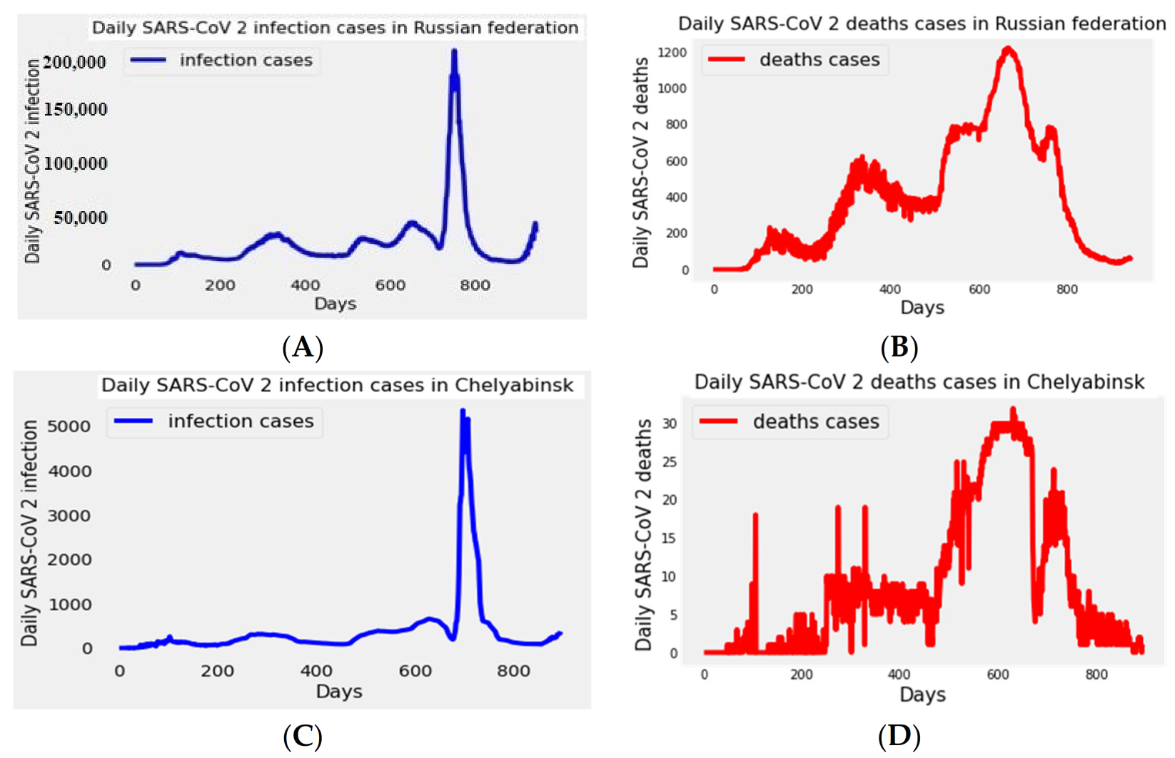
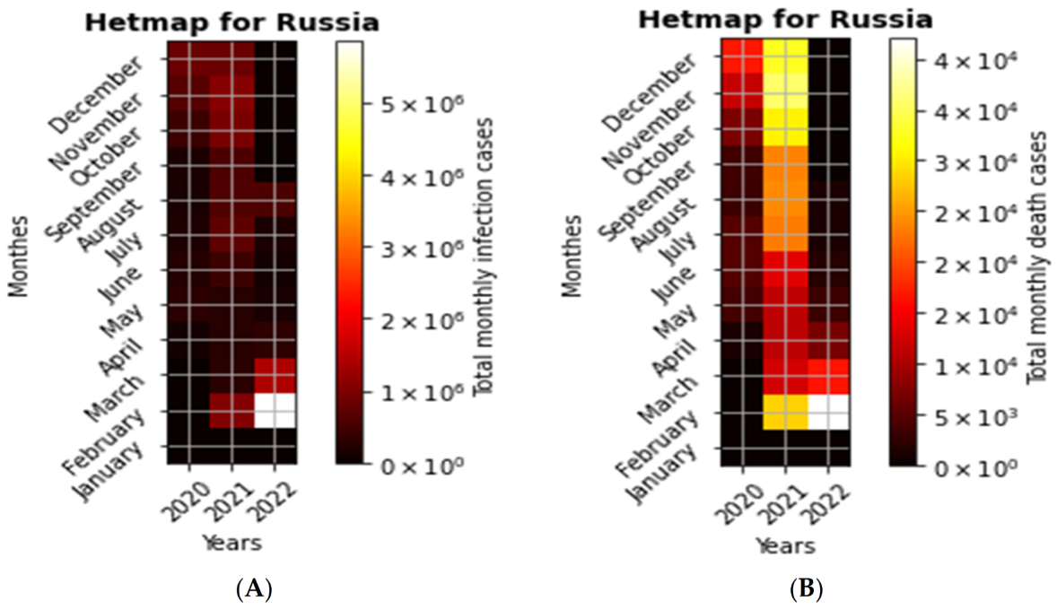
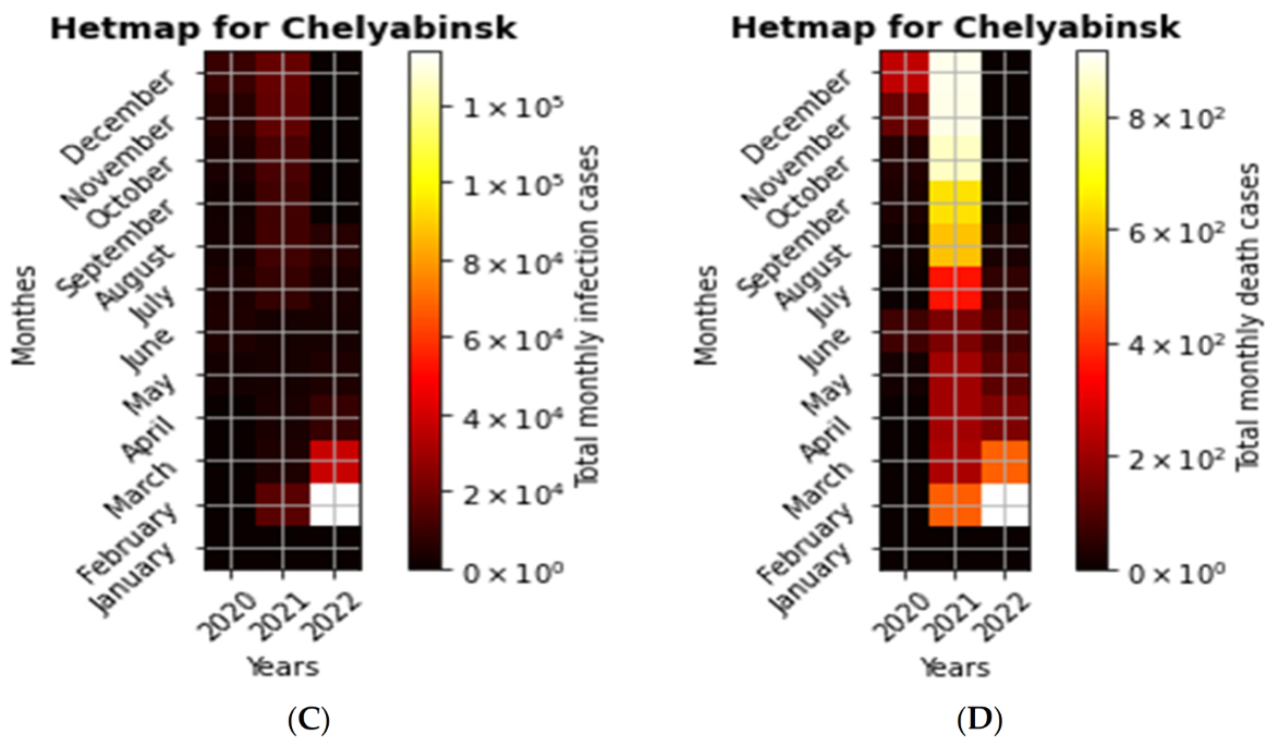
3. Data and Materials

When preparing data, deep learning faces some issues with long sequences in the database [36]. For the first problem, training is time-consuming and demands a lot of memory. Second problem, back-propagating extended sequences, results in an incorrectly trained model. Prepare and preprocess data before importing it into neural networks. Normalization and standardization problems are two aspects of data preparation. We used data normalization, a scaling procedure, to set the mean and standard deviation to 0 and 1, respectively [37]. We used daily data on SARS-CoV-2 infection and death cases in the Russian Federation and Chelyabinsk region. The dataset was obtained from the official website of the World Health Organization between the dates of 22 January 2020 and 23 August 2022. The dataset is then further prepared in such a way that the first eighty percent of the datasets are used for training purposes while the remaining twenty percent of the datasets are used for testing purposes (the last 20% of this dataset approximates the last 6 months (last 190 days)). The training dataset was used to train and improve the models, and 20% of the training data was utilized to analyze if the models were overfitting or underfitting the data. The performance of the model is evaluated with the help of the test set. Ref [38] provides both the method and the daily SARS-CoV-2 infection and death case data. Both of these can be accessed from our source.

Figure 1 showed a visual depiction of SARS-CoV-2 infection cases (left panel) and death cases (right panel) in Russia and Chelyabinsk repeatedly (Figure 1A,C). Figure 1A shows that the maximum month for total infection cases in Russia is February 2021. Figure 1C shows the same situation for infection cases in Chelyabinsk that same month (February 2021 and 2022). It had close to 100 thousand infection cases in 2022 when the mutant omicron appeared. We also note an upward trend in the development of death cases in Russia and Chelyabinsk (Figure 1B,D), with the emergence of volatility in death cases during the period. Figure 1B shows that the maximum month for total death cases in Russia is February 2022; Figure 1D shows that the maximum total number of death cases in November, December, and February in Chelyabinsk exceeded 800 death cases in November 2021. Then we find a decrease in the death cases after this month as a result of precautionary measures taken by both regions. One of the clear patterns in the visual is a similar trend in cases and death in both Russia and Chelyabinsk, which shows the unification of anti-SARS-CoV-2 policies. Using a heatmap enables us to extract some features from the SARS-CoV-2 data.

Figure 2 presents the heatmap for total monthly infection and death cases. Figure 2A shows that the maximum month for total infection cases in Russia is February 2021, and the same month in 2022 had close to 5 million infection cases in 2022 when the mutant omicron appeared. Figure 2B shows that the maximum month for total death cases in Russia is February 2022, and the same situation occurred in February 2021 when the mutant delta appeared. Figure 2C shows the same situation for infection cases in Chelyabinsk that same month (February 2021 and 2022). It had close to 100 thousand infection cases in 2022 when the mutant omicron appeared. Figure 2D shows that the maximum total number of death cases in November, December, and February in Chelyabinsk exceeded 800 death cases in November 2021.

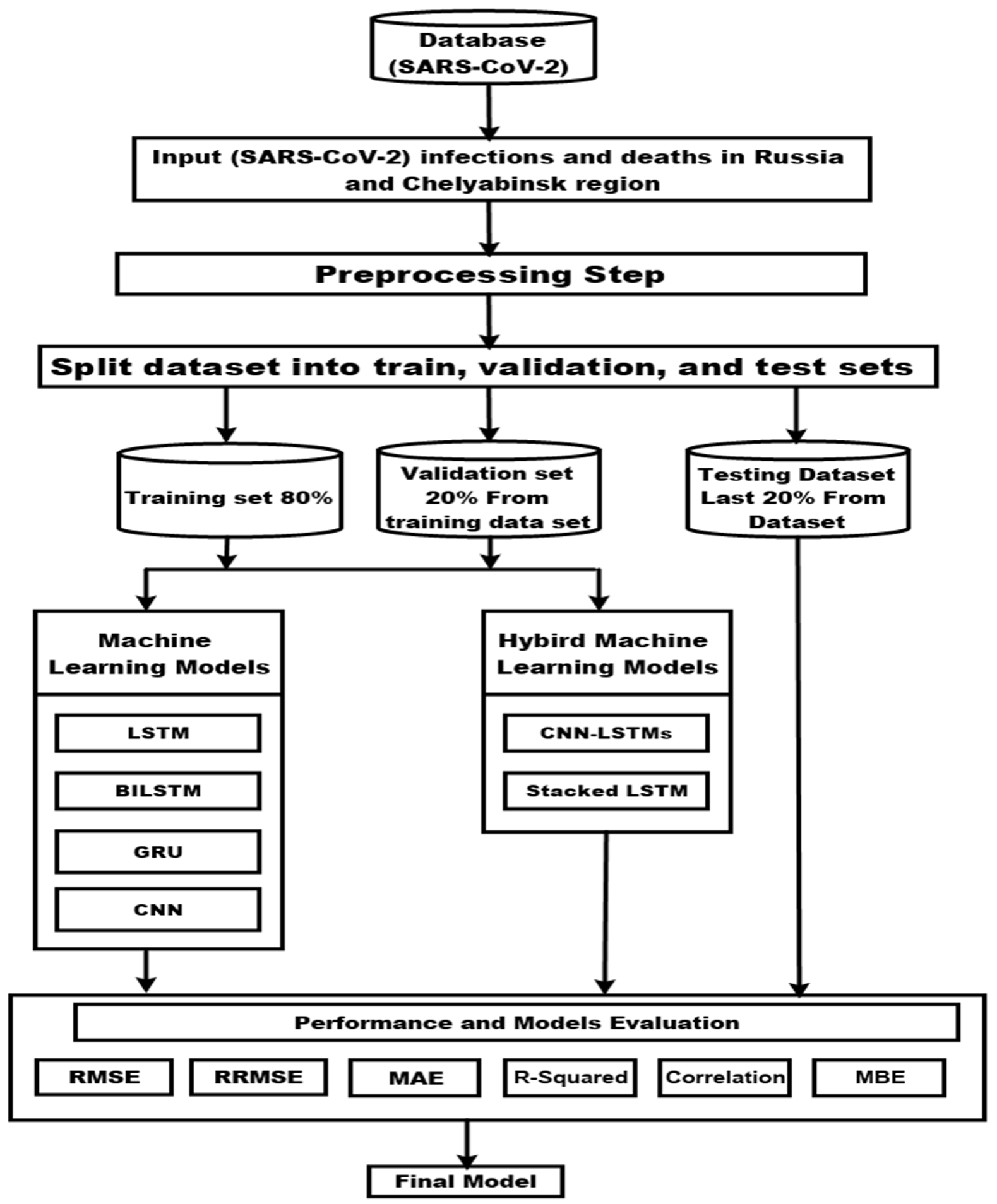
4. Proposed Framework Algorithm and Methodology

The mechanism that underlies our proposed approach for modeling and forecasting SARS-CoV-2 is depicted in Figure 3. The subsequent stages are carried out.

4.1. Proposed Framework Algorithm

First step → Input time series data for daily infection and death cases into our algorithm. Then input parameters for the deep learning model (number of neural networks, number of epochs, Loss Function, and optimizer) start running the algorithm.

Second step → preprocessing step, training takes time and memory. Second, back-propagating extended sequences create a poorly trained model. Before importing data into neural networks, prep it. Normalization and standardization are data prep steps. Using data normalization, we set the mean and standard deviation to 0 and 1, respectively.

Third step → Separate the dataset into training, validation, and testing. SARS-CoV-2 infection and death cases. From 22 January 2020 to 23 August 2022, WHO website data was collected. We test our model using 20% of this dataset (the last 190 days). The dataset is divided such that 80% is used for training and 20% for testing. We utilized the training dataset to train and improve the models and 20% to test overfitting and underfitting. Test set is used to evaluate model performance.

Fourth step → Modeling In this stage, we execute our algorithm for LSTM, LSTMs (stacked LSTM), BDLSTM (Bidirectional LSTM), ConvLSTMs, and other forecasting models.

Fourth step → Performance and Models Evaluation

Fifth step → Forecasting using best models

4.2. Methodology

(A) 

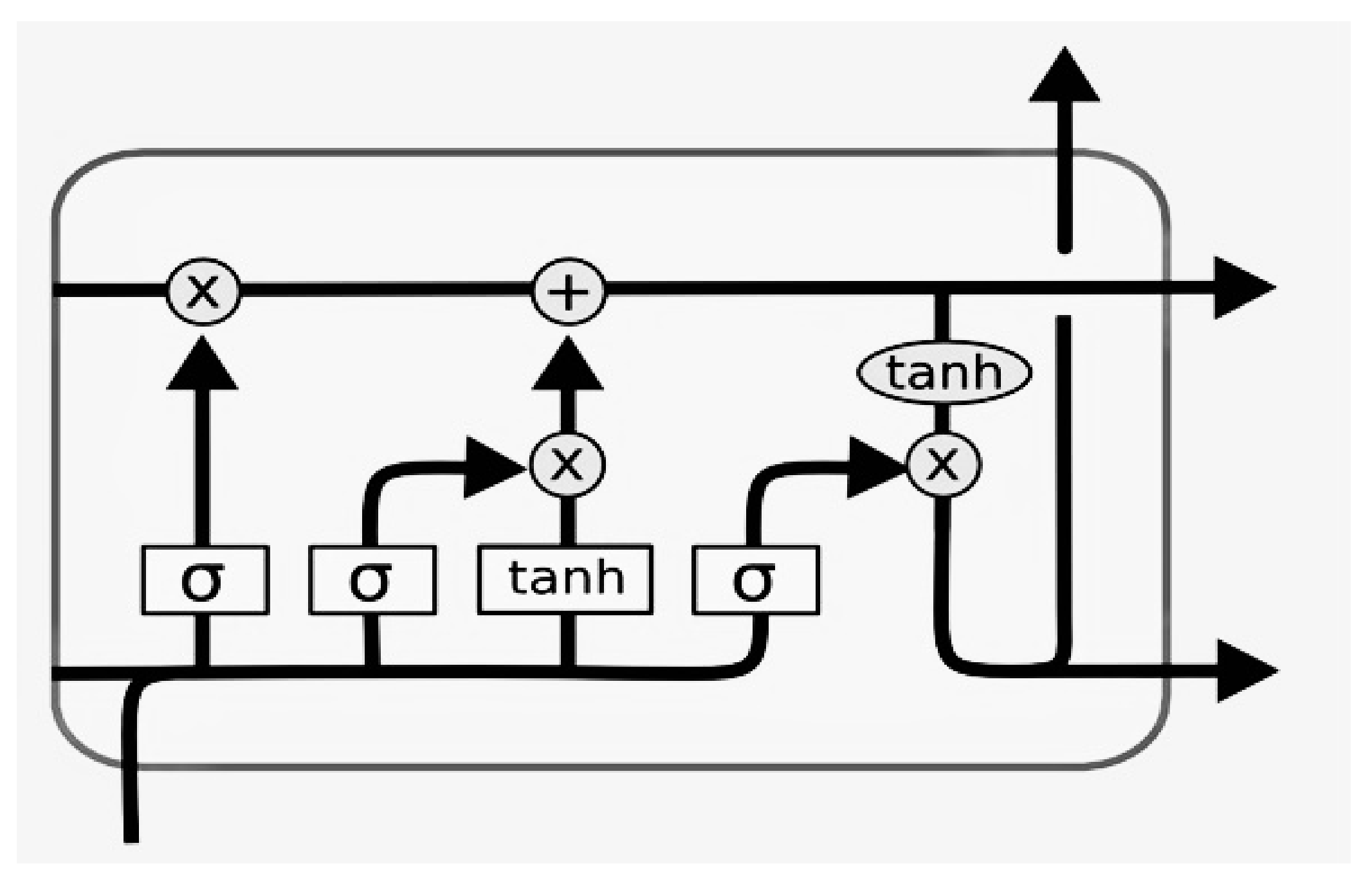
LSTM Model (long short-term memory model)

One of the first and most successful techniques for addressing vanishing gradients came in the form of long short-term memory (LSTM) due to [39].

The (long-term memory) part comes after simple recurrent neural networks have long-term memory in the form of weights. Weights change slowly during training, encoding general knowledge about the data. Moreover, the other part (short-term memory) is due to ephemeral activations, which go from each node to successive nodes. The LSTM model introduces an intermediate type of storage via the memory cell. A memory cell is a complex unit built from simpler nodes in a specific communication pattern with a new inclusion of multiplex nodes. A generalized LSTM unit consists of three gates (input, output, and a forget). The LSTM transition equations are given as follows [40].

Input gate: this gate makes the decision of whether or not the new information will be added to LSTM memory. This gate consists of two layers: (1) the sigmoid layer and (2) tanh layer. The first layer defines the values to be updated, and tanh layer creates a vector of new candidate values that will be added to LSTM memory. The output of these layers is calculated by:

$$i_t=\mathsf{\sigma }\left(W^i{x}_t+U^i{h}_{t-1}+b^i\right)$$

(1)

$$u_t=\tan \mathrm{h}\left(W^u{x}_t+U^u{h}_{t-1}+b^u\right)$$

(2)

where $i_t$: values updates, $u_t$: new candidate values, $\mathsf{\sigma }$: sigmoid layer (or nonlinear function), $x_t$: represents a sequence of length t, $b$: is a constant bias, $h$: represents RNN memory at time step t. $W$ and $U$ are weight matrices.

Forget gate: the sigmoid function of this gate is used to decide what information to remove from LSTM memory. This decision is mainly made based on the value of $h$ and$x_t$. The output of this gate is $f$, which is the value between 0 and 1, where 0 indicates completely eliminating the acquired value, and 1 indicates that the entire value is preserved. This output is calculated as:

$$f_t=\mathsf{\sigma }\left(W^f{x}_t+U^f{h}_{t-1}+b^f\right)$$

(3)

where $f_t$: values updates, $\mathsf{\sigma }$: sigmoid layer (or nonlinear function), $x_t$: represents a sequence of length t, $b$: is a constant bias, $h$: represents RNN memory at time step t. $W$ and $U$ are weight matrices.

Input gate: this gate first uses a sigmoid layer to decide which part of LSTM memory contributes to output. Next, it implements a nonlinear tanh function to set values between −1, 1. Finally, the result is multiplied by output of the sigmoid layer. The following equation represents the formulas for calculating output:

$$o_t=\mathsf{\sigma }\left(W^o{x}_t+U^o{h}_{t-1}+b^o\right)$$

(4)

$$h_t=o_t{\mathit{tanh}}_t{c}_{t-1}$$

(5)

where $o_t$: is an output gate, $h_t$: is represented as a value between [1, −1].

Combining these two layers provides an update to LSTM where the current value is forgotten using forget layer by doubling the old value $c_{t-1}$ followed by adding candidate value $i_t{u}_t$, The following equation represents its mathematical equation:

$$c_t=i_t{u}_t+f_t{c}_{t-1}$$

(6)

where $c_t$: is a memory cell. $f_t$ are the results of forget gate, which is a value between 0 and 1 where 0 indicates completely rid-of value; 1 implies completely preserved value. The hypothetical combination between these units is illustrated in Figure 4

(B) 

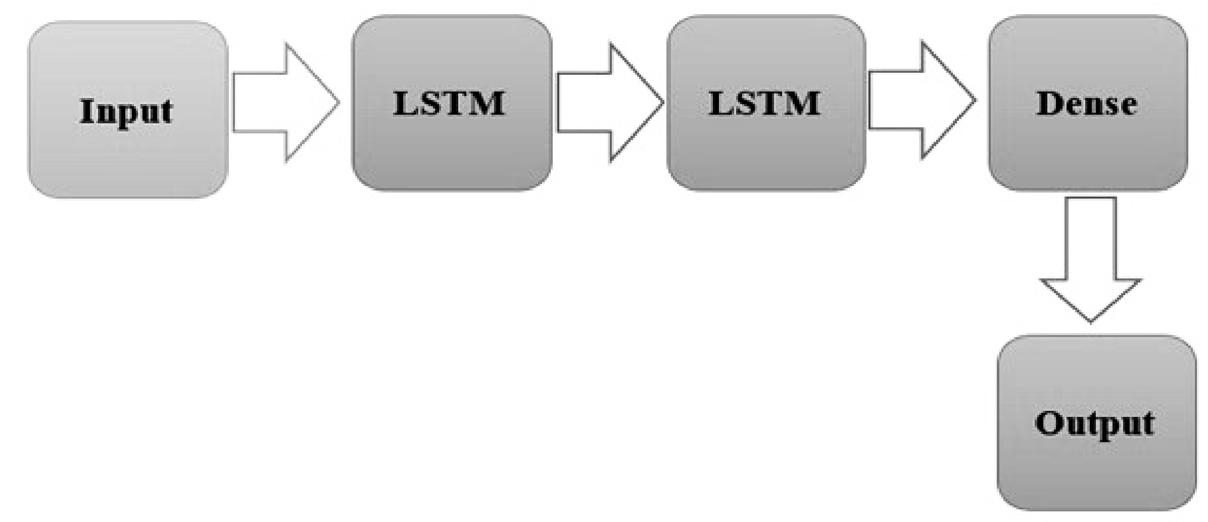
Stacked LSTM (Stacked long-short-term memory model)

Stacked LSTM model is an extension of LSTM model as it consists of multiple hidden layers where each layer contains multiple memory cells. It was introduced by [41]. They found that the depth of network was more important than the number of memory cells in a given layer to model skill layer for modeling the skill.

A stacked LSTM architecture can be defined as an LSTM model comprised of multiple LSTM layers. It provides a sequence output rather than a single value output to LSTM layer below. Specifically, one output per input time step rather than one output time step for all input time steps. This is illustrated in Figure 5.

(C) 

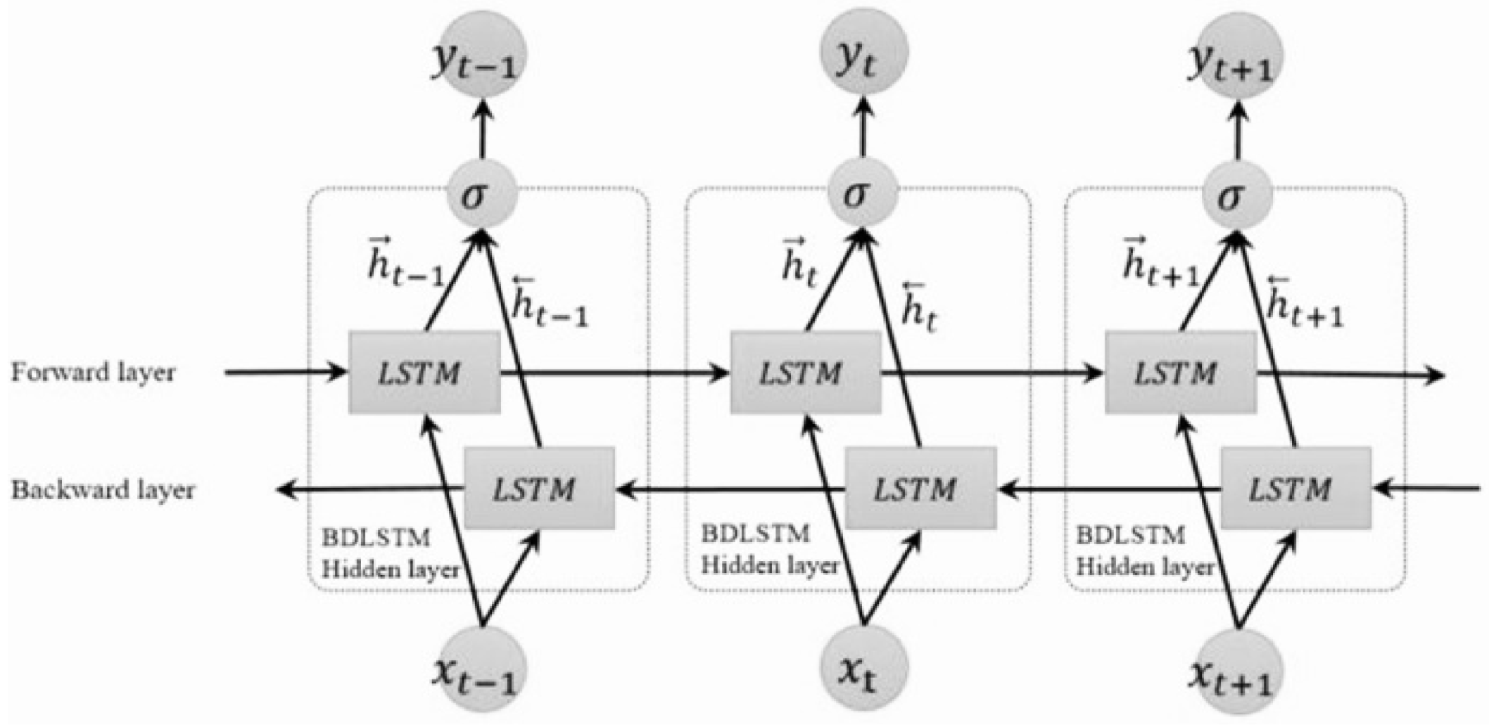
Bi LSTM model (Bidirectional long-short-term memory model)

Bi LSTM model put two independent RNNs together. This architecture allows network to obtain back-and-forth information about the sequence at each time step [42].

Using Bi LSTM will run inputs in two ways, one from past to future and one from future to past; where this approach differs from unidirectional is that in LSTM running backward, you keep information from the future and using the two hidden states together are able at any time to hold the information from the past and future. Calculating the output y at time t is illustrated in Figure 6.

$$y_t=\mathsf{\sigma }\left(W_y\left[h_t^{\to },h_t^{\leftarrow }\right]+b_y\right)$$

(7)

where $\mathsf{\sigma }$ is nonlinear function, $W_y$: are weight matrices that are used in deep learning models, $b_y$: is a constant bias. $h_t$: are hidden states.

Is illustrated in Figure 5:

Figure 6 shows us how Bi LSTM model works, as it shows information sent from past and future time series (green color), from inputs $x_t$, which are collected in hidden layers $h_t$ and extract features through nonlinear function σ to predict moment $y_t$.

(D) 

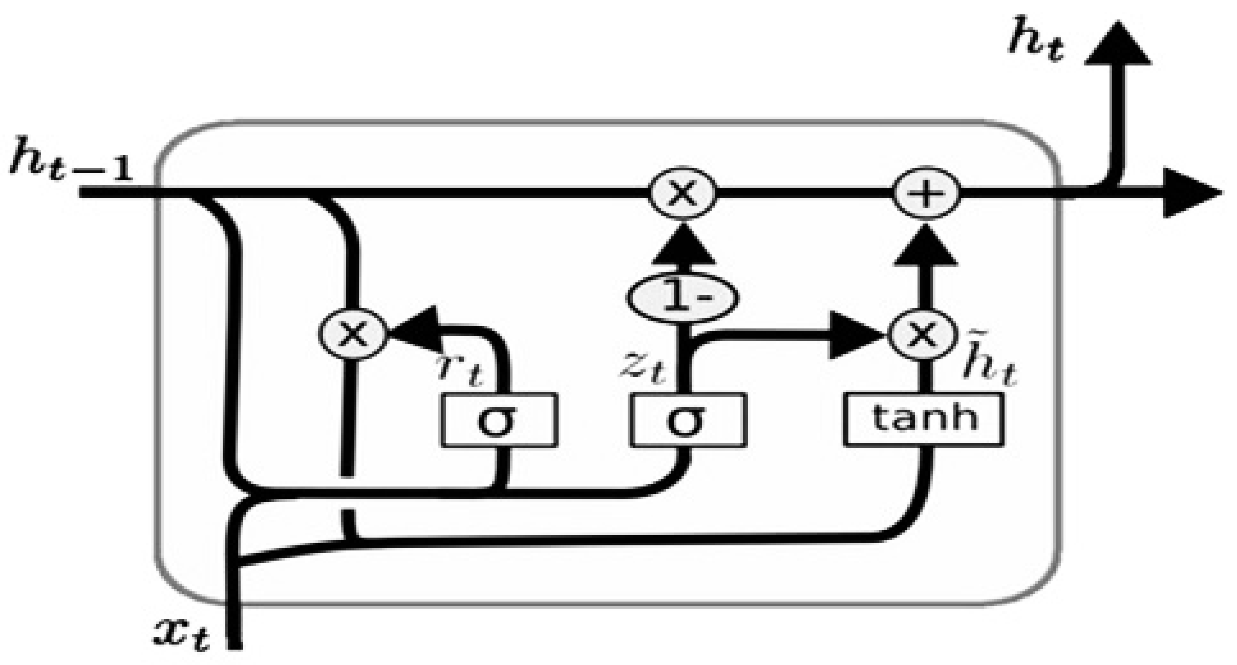
GRU model (Gated Recurrent Unit model)

Gated Recurrent Unit (GRU) is an advanced and more improved version of LSTM. It is also a type of recurrent neural network. It uses less hyper parameters because of reset gate and update gate in contrast to three gates of LSTM. Update gate and reset gate are basically vectors and are used to decide which information should be passed to the output [43]. The reset gate controls how much of the previous state we need to remember. From there, update gate will allow us to control whether the new state is a copy of old state. Two gate outputs are given by two fully connected layers with sigmoid activation function; Figure 7 shows the inputs for both reset and update gates in GRU. Mathematically, output is calculated as follows:

$$r_t=\mathsf{\sigma }\left(W^r{x}_t+U^r{h}_{t-1}+b^r\right)$$

(8)

$$z_t=\mathsf{\sigma }\left(W^z{x}_t+U^z{h}_{t-1}+b^z\right)$$

(9)

where $r_t$: is reset gate, $z_t$: is update gate, $\mathsf{\sigma }$: sigmoid activation function, $W$ and $U$ are weight parameters, $h_{t-1}$: the hidden state of the previous time step, $b$: is a constant bias. Next, we combine the reset gate with the regular refresh mechanism; it is given mathematically according to following equation:

$$i_t=\mathsf{\sigma }\left(W^i{x}_t+U^i{h}_{t-1}+b^i\right)$$

(10)

Which leads to the next candidate hidden state:

$$a_t=\tan \mathrm{h}\left(w{x}_t+r_t{U}^i{h}_{t-1}+b^h\right)$$

(11)

where: $a_t$: candidate hidden state, $\tan \mathrm{h}$: activation function, $w$ and $U$ are weight parametres, $r_t$: is reset gate, $h_{t-1}$: the hidden state of the previous time step, $b$: is a constant bias. Finally, we need to incorporate the effect of update gate. This determines how closely new hidden state is with old state versus how similar it is to new candidate state. Update gate can be used for this propose, simply by taking element-wise convex combinations of $h_t$ and $h_{t-1}$. This leads to final update equation for GRU:

$$h_t=z_t{h}_{t-1}+\left(1-z_t\right)a_t$$

(12)

where $z_t$: update gate, $r_t$: reset gate, $a_t$: activation function, $h_t$: hidden state output gate. The following Figure 7 illustrates this model:

(E) 

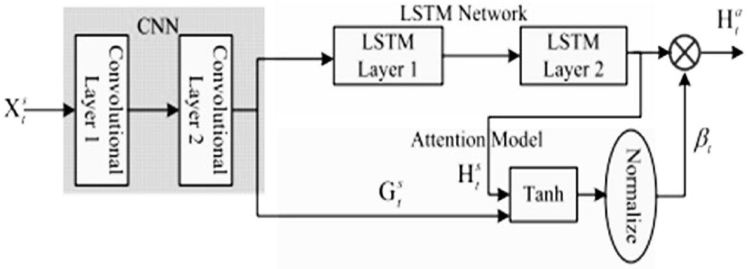
Conv and CNN-LSTM Model

The convolutional neural network consists of two convolutional layers; this allows for spatial advantage extraction. Where one-dimensional convolution operation is performed over the flow of data $x_t^s$ at each time step t., a one-dimensional convolution kernel filter is used to acquire the local perceptual domain by a sliding filter [44]. The process of convolution kernel filter can be expressed as follows:

$$Y_t^s=\sigma \left(W_s\ast x_t^s+b_s\right)$$

(13)

where $Y_t^s$: output of convolutional layer, $W_s$: weights of the filter, $x_t^s$: input traffic flow at time t, $\sigma$: activation functions.

CNN-LSTM Model is combination of Conv and LSTM; the input of CNN-LSTM is a spatial-temporal traffic flow matrix $x_t^s$, as follows [2]:

$$x_t^s=\left[\begin{array}{c}{x}_{t-n}^s\\ x_{t-\left(n-1\right)}^s\\ ⋮\\ x_t^s\end{array}\right]\left[\begin{array}{cccc}{f}_{t-n}^1& f_{t-\left(n-1\right)}^1& \dots & f_t^1\\ f_{t-n}^2& f_{t-\left(n-1\right)}^2& \cdots & f_t^2\\ ⋮& ⋮& \ddots & ⋮\\ f_{t-n}^m& f_{t-\left(n-1\right)}^m& \cdots & f_t^m\end{array}\right]$$

(14)

where $x_t^s=f_t^1\dots f_t^m$: denotes the traffic flow of the prediction region at time t, which represents the historical traffic flow of the POI to be predicted and its neighbors. As shown in Figure 8:

Figure 8 shows us how CNN-LSTM model works; this is performed by adding CNN layer on the front end (left panel) followed by LSTM layers with a dense layer on output (right panel). CNN model works to extract features, and LSTM model works to interpret over time steps.

(F) 

Adam Optimization Algorithm

Stochastic gradient descent is extended by Adam optimization in order to update network weights in a more efficient manner. The method of adaptive moment estimation is used in stochastic optimization. This makes it possible for the rate of learning to adjust over the course of time, which is a vital concept to grasp, given that Adam also demonstrates this phenomenon. Adam is the result of combining the two variables (Momentum and RMSprop) as shown in Algorithms 1, which presents a method in greater detail and also Pseudo-code 1.

Adam proposed algorithm for stochastic optimization and for a slightly more efficient order of computation. $g_t^2$ indicates the elementwise square $g_t\odot g_t$. Good default settings for the tested machine learning problems are α = 0.001, ${\beta }_1$ = 0.9, ${\beta }_2$ = 0.999, and ϵ = ${10}^{-8}$. All operations on vectors are element-wise. With ${\beta }_1^t$ and ${\beta }_2^t$ we denote ${\beta }_1$ and ${\beta }_2$ to the power t [19].

Algorithms 1: Adam algorithm for stochastic optimization [19].

Require: $a:$ Stepsize Require: ${\beta }_1,{\beta }_2\in \left[0,1\right):$Exponential decay rates for the moment estimates Require:$f\left(\theta \right):$Stochastic objective function with parameters $\theta$ Require:${\theta }_0:$ Initial parameter vector $m_0\leftarrow$      0(Initialize 1st moment vector) $v_0\leftarrow$      0(Initialize 2nd moment vector) $t\leftarrow$      0(Initialize timestep) while $\theta$ not converged do      $t+t_1$      $g_t\leftarrow {\nabla }_{\theta }{f}_t\left({\theta }_{t-1}\right)$ (Get gradients w.r.t. stochastic objective at timestep $t$)      $mt\leftarrow {\beta }_1·m_{t-1}+\left(1-{\beta }_1\right)·g_t$ (Update biased first moment estimate)      $vt\leftarrow {\beta }_2·v_{t-1}+\left(1-{\beta }_2\right)·g_t^2$ (Update biased second raw moment estimate)      ${\widehat{m}}_t\leftarrow m_t/\left(1-{\beta }_1^t\right)$ (Compute bias-corrected first moment estimate)      ${\widehat{v}}_t\leftarrow v_t/\left(1-{\beta }_2^t\right)$ Compute bias-corrected second raw moment estimate)      ${\theta }_t\leftarrow {\theta }_{t-1}-a·{\widehat{m}}_t/(\sqrt{{\widehat{v}}_t}+ϵ$(Update parameters)      end while      return ${\theta }_t$ (Resulting parameters

Adaptive Moment Estimation (Adam) Pseudo-code: Adam algorithm for stochastic optimization Note: We have two separate beta coefficients → one for each optimization part. We implement bias correction for each gradient

On iteration t: Compute dW, db for current mini-batch # #Momentum v_dW = beta1 * v_dW + (1 − beta1) dW v_db = beta1 * v_db + (1 − beta1) db v_dW_corrected = v_dw/(1 − beta1 ** t) v_db_corrected = v_db/(1 − beta1 ** t) # #RMSprop s_dW = beta * v_dW + (1 − beta2) (dW ** 2) s_db = beta * v_db + (1 − beta2) (db ** 2) s_dW_corrected = s_dw/(1 − beta2 ** t) s_db_corrected = s_db/(1 − beta2 ** t) # #Combine W = W − alpha * (v_dW_corrected/(sqrt(s_dW_corrected) + epsilon)) b = b − alpha * (v_db_corrected/(sqrt(s_db_corrected) + epsilon)) Coefficients alpha: the learning rate. 0.001. beta1: momentum weight. Default to 0.9. beta2: RMSprop weight. Default to 0.999. epsilon: Divide by Zero failsave. Default to 10 ** −8.

(G) 

Performance indicators

To compare the prediction performance of the three models used:

Calculating root mean square error (RMSE) between the estimated data and actual data:

$$\mathrm{RMSE} =\sqrt{\frac{{{\displaystyle \sum }}_{t =1}^n{\left(\widehat{y_t}-y_t\right)}^2}{n}}$$

(15)

where$\widehat{y_t}$: the forecast value, $y_t$: the actual value, $n$: number of fitted observed.

Calculating relative root mean square error (RRMSE):

$$\mathrm{RRMSE}=\sqrt{\frac{\frac{1}{n}{{\displaystyle \sum }}_{t =1}^n{\left(\widehat{y_t}-y_t\right)}^2}{{{\displaystyle \sum }}_{t=1}^n{\left(\widehat{y_t}\right)}^2}}$$

(16)

Calculating mean absolute error (MAE):

$$\mathrm{MAE}=\frac{1}{n}{\displaystyle \sum }_{t=1}^n\left|y_t-{\widehat{y}}_t\right|$$

(17)

Calculating mean bias error (MBE):

$$\mathrm{MBE}=\frac{{{\displaystyle \sum }}_{t=1}^n(y_t-{\widehat{y}}_t)}{n}$$

(18)

Calculating Coefficient of correlation (R):

$$\mathrm{R}=\frac{Cov\left(y_t,{\widehat{y}}_t\right)}{\sqrt{V\left(y_t\right) V\left({\widehat{y}}_t\right)}}$$

(19)

Calculating Coefficient of determination (R Square):

$${\mathrm{R}}^2=1-\frac{{{\displaystyle \sum }}_{t=1}^n{\left({\widehat{y}}_t-{\overline{y}}_t\right)}^2}{{{\displaystyle \sum }}_{t=1}^n{\left(y_t-{\overline{y}}_t\right)}^2}$$

(20)

The model that has the least values of (RMSE—RRMSE—MAE—MBE) and greater values of (R–R-Square) is the best model.

5. Results

To prove the effectiveness and superiority of the proposed approach, several experiments were conducted to predict SARS-CoV-2. Firstly, a set of baseline experiments were conducted using six base models, including LSTM, BDLSTM, GRU, LSTMs, and CONVLSTMs. The results of these models were compared to the achieved results using the Bi-LSTM, LSTM, CNN, and CNN-LSTMs algorithm for daily infection and death for SARS-CoV-2 in Russia and Chelyabinsk, respectively.

Table 1. Comparison of six methods evaluation testing 20% SARS-CoV-2 daily infection and death cases in Russian federation and Chelyabinsk.

Model	RMSE	RRMSE	MAE	R2	r	MBE
(SARS-CoV-2)Infection Cases in Russia
LSTM	9126.42	0.40	3653.27	0.93	1.00	3023.27
Stacked LSTM	35,612.77	1.56	12,646.76	−0.03	0.26	−10,796.24
BDLSTM	2611.48	0.11	1417.74	0.99	1.00	−59.11
GRU	13,105.75	0.57	4223.04	0.86	0.97	−3299.01
Conv	3397.80	0.33	1936.18	0.86	0.96	−1277.09
CNN-LSTMs	2583.41	0.25	1717.80	0.92	0.98	−1315.08
(SARS-CoV-2)Death Cases in Russia
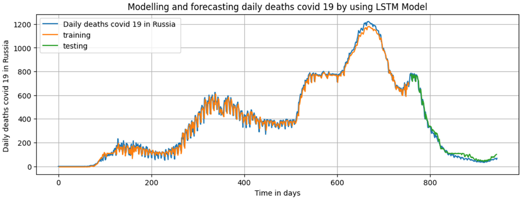
LSTM	24.46	0.12	20.19	0.99	1.00	13.85
Stacked LSTM	32.29	0.15	27.62	0.98	1.00	22.80
BDLSTM	24.98	0.12	20.97	0.99	1.00	16.61
GRU	27.07	0.13	23.33	0.99	1.00	19.77
Conv	88.80	0.70	46.65	0.37	0.99	39.03
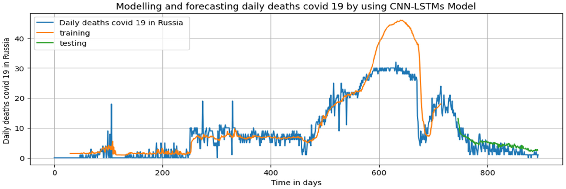
CNN-LSTMs	58.11	0.46	37.69	0.73	0.99	16.52
(SARS-CoV-2)Infection Cases in Chelyabinsk region
LSTM	160.23	0.43	59.46	0.91	1.00	57.78
Stacked LSTM	583.25	1.55	188.00	0.14	0.03	−177.87
BDLSTM	64.47	0.17	25.46	0.99	1.00	21.97
GRU	64.98	0.17	25.38	0.99	1.00	20.51
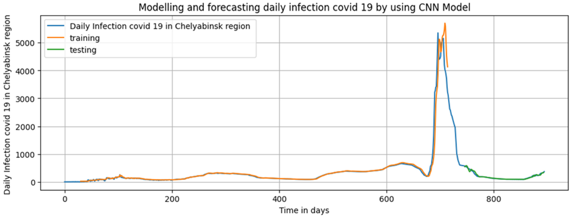
Conv	24.69	0.13	14.36	0.96	0.98	3.86
CNN-LSTMs	122.46	0.65	86.77	−0.02	0	−19.01
SARS-CoV-2Death Cases in Chelyabinsk region
LSTM	1.84	0.35	1.44	0.88	0.94	0.22
Stacked LSTM	1.91	0.37	1.46	0.87	0.94	0.15
BDLSTM	2.03	0.39	1.63	0.85	0.94	0.68
GRU	1.79	0.35	1.39	0.89	0.94	−0.03
Conv	2.83	0.90	2.19	−0.44	0.75	1.87
CNN-LSTMs	1.60	0.51	1.29	0.54	0.78	0.63

presents the results of the testing for each of the base models along with the proposed approach based on the adopted evaluation criteria.

As presented in the table, the proposed approach could achieve the best values over all the evaluation criteria, which confirms the superiority of the proposed approach. The achieved RMSE on the test set using the proposed approach BDLSTM for infection cases of SARS-CoV-2 in Russia is (2611.48). In addition, RRMSE, MAE, R², r, and MBE of the test set using the proposed approach BDLSTM is (0.11), (1417.74), (0.99), (1), and (−59.11). These values prove the effectiveness of the proposed approach. The achieved RMSE on the test set using the proposed approach LSTM for death cases of SARS-CoV-2 in Russia is (24.46). In addition, RRMSE, MAE, R², r, and MBE of the test set using the proposed approach LSTM is (0.12), (20.19), (0.99), (1), and (13.85). These values prove the effectiveness of the proposed approach. The achieved RMSE on the test set using the proposed approach Conv for infection cases of SARS-CoV-2 in the Chelyabinsk region is (24.69). In addition, RRMSE, MAE, R², r, and MBE of the test set using the proposed approach Conv are (0.13), (14.36), (0.96), (0.98), and (3.86). These values prove the effectiveness of the proposed approach. The achieved RMSE on the test set using the proposed approach CNN-LSTMs for death cases of SARS-CoV-2 in the Chelyabinsk region is (1.60). In addition, RRMSE, MAE, R², r, and MBE of the test set using the proposed approach CNN-LSTMs are (0.51), (1.29), (0.54), (0.78), and (0.63). These values prove the effectiveness of the proposed approach.

Table 2. Descriptive statistics of SARS-CoV-2.

	Mean	S.E	Median	Mode	S.D	Kurtosis	Skewness	Mini	Max
Infection in Russia	20,002.25	940.40	11,409	0	28,908.88	18.08	4.015	0	202,211
Death in Russia	397.79	10.94	354	0	336.374	−0.50	0.70	0	1222
Infection Chelyabinsk	383.25	25.07	180	0	750.20	21.87	4.58	0	5354
Death Chelyabinsk	8.76	0.31	6	0	9.35	−0.11	1.06	0	32

shows us the large difference between the maximum and minimum values of all variables and thus affects the shape of the distribution. Thus, the estimators here (Mean, Median, Mode, and SD) are useless because they are breakdown points. We notice from the table that the largest difference is for the variable number of infections in Russia, from 0 to 202,211 cases, which leads to a kurtosis that gives a pointed top of the distribution as its value is much greater than three and a greater value for standard error (more difficulty in predicting), with the distribution skewed towards the right as the frequency of values greater than the average is greater for this variable. as the injury variable in Russia took 700 days to move from the lowest value to the largest value. The same thing happened for infection Chelyabinsk, with less difference between max and min values leading to less S.D. As for death cases, we notice a negative kurtosis, which indicates less volatility for both variables and, therefore, a smaller S.D than infection cases with a slight Skewness due to the convergence of the values from the arithmetic mean, and therefore, the cases of death are less developed than the cases of injury with the preventive measures that have been taken in these areas.

The table shows us that the best model for predicting SARS-CoV-2 infection cases in Russia is (BDLSTM) because it has the least values of (RMSE—RRMSE—MAE—MBE) and, therefore, the least difference between the real and estimated values using the model. We also note that the model is able to explain the volatility in a variable through the high value of the coefficient of determination (R Square = 99%); there is a perfect linear correlation between the estimated and actual values. As before, we note that the best model for SARS-CoV-2 death cases in Russia is (LSTM), and for SARS-CoV-2 infection cases in the Chelyabinsk region is (CONV), and for SARS-CoV-2 death cases in the Chelyabinsk region is (CNN-LSTMs). As these models achieve convergence between the actual and estimated values of the training and test data, noting their ability to capture extreme values (Maximum and Minimum value). This is illustrated by the following figures:

Figure 9 shows us the convergence of data on actual daily infection of SARS-CoV-2 in Russia with estimated using the BDLSTM model (training–testing), so we notice a great convergence between the actual and estimated data and the ability of the model to clarify volatility in infection of SARS-CoV-2 and capture structural points, and thus this model can be used to predict in daily infection of SARS-CoV-2 in Russia.

Figure 10 shows us the convergence of data on actual daily death SARS-CoV-2 in Russia with estimated using the LSTM model (training–testing), so we notice a great convergence between the actual and estimated data and the ability of model to clarity volatility in death SARS-CoV-2 and capture trends change and thus this model can be used to predict in daily death SARS-CoV-2 in Russia.

Figure 11 shows us the convergence of data on actual daily infection SARS-CoV-2 in the Chelyabinsk region estimated using the CNN model (training–testing), so we notice a great convergence between the actual and estimated data and the ability of the model to clarify volatility in SARS-CoV-2 infection and capture structural points, and thus this model can be used to predict in daily SARS-CoV-2 infection in the Chelyabinsk region.

Figure 12 shows us the convergence of data on actual daily death SARS-CoV-2 in the Chelyabinsk region with estimated using the CNN-LSTMs model (training–testing), so we notice a great convergence between the actual and estimated data and the ability of the model to clarify volatility in death SARS-CoV-2 and capture structural points, and thus this model can be used to predict in daily death SARS-CoV-2 in the Chelyabinsk region. The hyper-parameters for deep learning models are shown in

Table 3. Hyper-parameter setting for models.

Parameter	Infection in	Death	Infection	Death
Area	Russia	Russia	Chelyabinsk	Chelyabinsk
Model	BDLSTM	LSTM	Conv	ConvLSTMs
Activation function	Relu	Relu	Relu	Relu
Number of hidden units in LSTM layer	200	200	200	200
LSTM layer activation function	Relu	Relu	Relu	Relu
Timestep	2	2	2	10
Batch size	1	1	1	1
Optimizer	Adam	Adam	Adam	Adam
Learning rate	0.001	0.001	0.001	0.001
Loss function	MSE	MSE	MSE	MSE
Epochs	200	200	200	200

.

6. Conclusions and Future Research

In this study, a hybrid deep learning model’s algorithm was used to improve the performance of a standard LSTM network in the analysis and forecasting of SARS-CoV-2 infections and death cases in the Russian Federation and the Chelyabinsk region. This was accomplished by using a combination of traditional LSTM networks and hybrid deep learning models. In order to demonstrate that the strategy being offered is effective, a dataset is gathered for the purposes of analysis and prediction. The suggested method was evaluated by applying it to datasets obtained from an official data source that was representative of the Russian Federation and the Chelyabinsk region. The utilization of these six key performance indicators allows for the performance of the suggested methodology to be evaluated and analyzed. In addition, the performance of the suggested method is evaluated and compared to that of the other five prediction models in order to demonstrate that the proposed method is superior. The compiled data provided unmistakable evidence that the strategy being recommended (Hybrid Deep-Learning models) are not only successful but also significantly more advantageous and important. On the other hand, it serves as a reference for the health sector in Russia, in particular, as well as the World Health Organization (WHO), as well as, more generally, for the health sectors in other nations. As for future research directions, it is planned to enable medium- and long-term forecasting of time series in weakly structured situations, to develop mechanisms for correcting long-term forecasts, to force a set of forecasting models to account for forecasting quality in previous periods, and to consider the possibility of employing nonlinear forecasting models for weakly structured data. All of these, along with the use of additional criteria for the verification of the best models, can be used to expand and enhance the algorithm discussed in this study and create a new package in Python for modeling and forecasting not only SARS-CoV-2 data but any univariate-dimensional time series data.

References

- Chakraborty, I.; Maity, P. COVID-19 outbreak: Migration, effects on society, global environment and prevention. Sci. Total Environ. 2020, 728, 138882. [Google Scholar] [CrossRef] [PubMed]
- House, C.; Naseefa, N.; Palissery, S.; Sebastian, H. Corona viruses: A review on SARS, MERS and COVID-19. Microbiol. Insights 2021, 14, 11786361211002481. [Google Scholar]
- Sachs, J.; Schmidt-Traub, G.; Kroll, C.; Lafortune, G.; Fuller, G.; Woelm, F. Sustainable Development Report 2020: The Sustainable Development Goals and COVID-19 Includes the SDG Index and Dashboards; Cambridge University Press: Cambridge, UK, 2021. [Google Scholar]
- Shekerdemian, L.S.; Mahmood, N.R.; Wolfe, K.K.; Riggs, B.J.; Ross, C.E.; McKiernan, C.A.; Heidemann, S.M.; Kleinman, L.C.; Sen, A.I.; Hall, M.W.; et al. Characteristics and Outcomes of Children with Coronavirus Disease 2019 (COVID-19) Infection Admitted to US and Canadian Pediatric Intensive Care Units. JAMA Pediatr. 2020, 174, 868–873. [Google Scholar] [CrossRef]
- Li, J.-P.O.; Liu, H.; Ting, D.S.J.; Jeon, S.; Chan, R.V.P.; Kim, J.E.; Sim, D.A.; Thomas, P.B.M.; Lin, H.; Chen, Y.; et al. Digital technology, tele-medicine and artificial intelligence in ophthalmology: A global perspective. Prog. Retin. Eye Res. 2021, 82, 100900. [Google Scholar] [CrossRef]
- Bohr, A.; Memarzadeh, K. The rise of artificial intelligence in healthcare applications. Artif. Intell. Healthc. 2020, 25–60. [Google Scholar] [CrossRef]
- El-Sherif, D.M.; Abouzid, M.; Elzarif, M.T.; Ahmed, A.A.; Albakri, A.; Alshehri, M.M. Telehealth and Artificial Intelligence Insights into Healthcare during the COVID-19 Pandemic. Healthcare 2022, 10, 385. [Google Scholar] [CrossRef] [PubMed]
- Hossain, M.S.; Muhammad, G. Emotion recognition using deep learning approach from audio–visual emotional big data. Inf. Fusion 2019, 49, 69–78. [Google Scholar] [CrossRef]
- Abu Adnan Abir, S.M.; Islam, S.N.; Anwar, A.; Mahmood, A.N.; Than Oo, A.M. Building resilience against COVID-19 pandemic using artificial intelligence, machine learning, and IoT: A survey of recent progress. IoT 2020, 1, 506–528. [Google Scholar] [CrossRef]
- Pan, Y.; Zhang, L. Roles of artificial intelligence in construction engineering and management: A critical review and future trends. Autom. Constr. 2021, 122, 103517. [Google Scholar] [CrossRef]
- Ahin, M. Impact of weather on COVID-19 pandemic in Turkey. Sci. Total Environ. 2020, 728, 138810. [Google Scholar]
- World Health Organization. Available online: https://www.who.int/publications/m/item/weekly-epidemiological-update-on-covid-19 (accessed on 4 May 2022).
- Dutta, A.; Fischer, H.W. The local governance of COVID-19: Disease prevention and social security in rural India. World Dev. 2021, 138, 105234. [Google Scholar] [CrossRef] [PubMed]
- Hossain, F.; Clatty, A. Self-care strategies in response to nurses’ moral injury during COVID-19 pandemic. Nurs. Ethic- 2021, 28, 23–32. [Google Scholar] [CrossRef] [PubMed]
- Murhekar, M.V.; Bhatnagar, T.; Thangaraj, J.W.V.; Saravanakumar, V.; Kumar, M.S.; Selvaraju, S.; Vinod, A. SARS-CoV-2 seroprevalence among the general population and healthcare workers in India, December 2020–January 2021. Int. J. Infect. Dis. 2021, 108, 145–155. [Google Scholar] [CrossRef] [PubMed]
- Alassafi, M.O.; Jarrah, M.; Alotaibi, R. Time series predicting of COVID-19 based on deep learning. Neurocomputing 2022, 468, 335–344. [Google Scholar] [CrossRef]
- Tanıma, Ö.; Al-Dulaimi, A.; Harman, A.G.G. Estimating and Analyzing the Spread of COVID-19 in Turkey Using Long Short-Term Memory. In Proceedings of the 2021 5th International Symposium on Multidisciplinary Studies and Innovative Technologies (ISMSIT), Ankara, Turkey, 21–23 October 2021; pp. 17–26. [Google Scholar] [CrossRef]
- Ishfaque, M.; Dai, Q.; Haq, N.U.; Jadoon, K.; Shahzad, S.M.; Janjuhah, H.T. Use of Recurrent Neural Network with Long Short-Term Memory for Seepage Prediction at Tarbela Dam, KP, Pakistan. Energies 2022, 15, 3123. [Google Scholar] [CrossRef]
- Mostafa Salaheldin Abdelsalam, A.; Makarovskikh, T. The research of mathematical models for forecasting COVID-19 cases. In Proceedings of the International Conference on Mathematical Optimization Theory and Operations Research, Irkutsk, Russia, 5–10 July 2021; Springer: Cham, Switzerland. [Google Scholar]
- Mohamadou, Y.; Halidou, A.; Kapen, P.T. A review of mathematical modeling, artificial intelligence and datasets used in the study, prediction and management of COVID-19. Appl. Intell. 2020, 50, 3913–3925. [Google Scholar] [CrossRef]
- Duan, D.; Wu, X.; Si, S. Novel interpretable mechanism of neural networks based on network decoupling method. Front. Eng. Manag. 2021, 8, 572–581. [Google Scholar] [CrossRef]
- Agarwal, A.; Mishra, A.; Sharma, P.; Jain, S.; Ranjan, S.; Manchanda, R. Using LSTMfor the Prediction of Disruption in ADITYA Tokamak. arXiv 2020, preprint. arXiv:2007.06230. [Google Scholar]
- Abotaleb, M.S.; Makarovskikh, T. Analysis of Neural Network and Statistical Models Used for Forecasting of a Disease Infection Cases. In Proceedings of the 2021 International Conference on Information Technology and Nanotechnology (ITNT), Samara, Russia, 20–24 September 2021; pp. 1–7. [Google Scholar] [CrossRef]
- Makarovskikh, T.; Abotaleb, M. Comparison between Two Systems for Forecasting COVID-19 Infected Cases. In Computer Science Protecting Human Society Against Epidemics. ANTICOVID 2021. IFIP Advances in Information and Communication Technology; Byrski, A., Czachórski, T., Gelenbe, E., Grochla, K., Murayama, Y., Eds.; Springer: Cham, Switzerland, 2021; Volume 616. [Google Scholar] [CrossRef]
- Makarovskikh, T.; Salah, A.; Badr, A.; Kadi, A.; Alkattan, H.; Abotaleb, M. Automatic classification Infectious disease X-ray images based on Deep learning Algorithms. In Proceedings of the 2022 VIII International Conference on Information Technology and Nanotechnology (ITNT), Samara, Russia, 23–27 May 2022; pp. 1–6. [Google Scholar] [CrossRef]
- Darwish, O.; Tashtoush, Y.; Bashayreh, A.; Alomar, A.; Alkhaza’Leh, S.; Darweesh, D. A survey of uncover misleading and cyberbullying on social media for public health. Clust. Comput. 2022, 1–27. [Google Scholar] [CrossRef]
- Tabik, S.; Gomez-Rios, A.; Martin-Rodriguez, J.L.; Sevillano-Garcia, I.; Rey-Area, M.; Charte, D.; Guirado, E.; Suarez, J.L.; Luengo, J.; Valero-Gonzalez, M.A.; et al. COVIDGR Dataset and COVID-SDNet Methodology for Predicting COVID-19 Based on Chest X-Ray Images. IEEE J. Biomed. Health Inform. 2020, 24, 3595–3605. [Google Scholar] [CrossRef]
- Aboubakr, H.A.; Amr, M. On improving toll accuracy for covid-like epidemics in underserved communities using user-generated data. In 1st ACM SIGSPATIAL International Workshop on Modeling and Understanding the Spread of COVID-19; ACM: New York, NY, USA, 2020. [Google Scholar]
- Tashtoush, Y.; Alrababah, B.; Darwish, O.; Maabreh, M.; Alsaedi, N. A Deep Learning Framework for Detection of COVID-19 Fake News on Social Media Platforms. Data 2022, 7, 65. [Google Scholar] [CrossRef]
- Biswas, P.; Saluja, K.S.; Arjun, S.; Murthy, L.; Prabhakar, G.; Sharma, V.K.; Dv, J.S. COVID-19 Data Visualization through Automatic Phase Detection. Digit. Gov. Res. Pract. 2020, 1, 1–8. [Google Scholar] [CrossRef]
- Karajeh, O.; Darweesh, D.; Darwish, O.; Abu-El-Rub, N.; Alsinglawi, B.; Alsaedi, N. A classifier to detect informational vs. non-informational heart attack tweets. Future Internet 2021, 13, 19. [Google Scholar] [CrossRef]
- Zhang, Y.; Liao, Q.; Yuan, L.; Zhu, H.; Xing, J.; Zhang, J. Exploiting Shared Knowledge from Non-COVID Lesions for Annotation-Efficient COVID-19 CT Lung Infection Segmentation. IEEE J. Biomed. Health Inform. 2021, 25, 4152–4162. [Google Scholar] [CrossRef]
- Lin, H.Y.; Moh, T.-S. Sentiment Analysis on COVID Tweets Using COVID-Twitter-BERT with Auxiliary Sentence Approach. In 2021 ACM Southeast Conference, Virtual, 15–17 April 2021; ACM: New York, NY, USA, 2021. [Google Scholar] [CrossRef]
- Salamatov, A.A.; Davankov, A.Y.; Malygin, N.V. Socio-economic consequences of the COVID-19 Pandemic: The quality of Life of the Population in the Chelyabinsk Region in comparison with the Ural Federal District and Russia. Bull. Chelyabinsk State Univ. 2022, 72–80. [Google Scholar] [CrossRef]
- Karasu, S.; Altan, A. Crude oil time series prediction model based on LSTM network with chaotic Henry gas solubility optimization. Energy 2022, 242, 122964. [Google Scholar] [CrossRef]
- Khan, S.D.; AlArabi, L.; Basalamah, S. Toward Smart Lockdown: A Novel Approach for COVID-19 Hotspots Prediction Using a Deep Hybrid Neural Network. Computers 2020, 9, 99. [Google Scholar] [CrossRef]
- Ali, P.J.M.; Faraj, R.H.; Koya, E. Data normalization and standardization: A technical report. Mach Learn. Technol. Rep. 2014, 1, 1–6. [Google Scholar]
- Abotaleb, M. Hybrid Deep Learning Algorithm. Available online: https://github.com/abotalebmostafa11/Hybrid-deep-learning-Algorithm (accessed on 26 September 2022).
- Hochreiter, H.; Schmidhuber, J. Long short term memory. Neural Comput. 1997, 9, 1735–1780. [Google Scholar] [CrossRef]
- Huynh, H.; Dang, L.; Duong, D. A new model for stock price movements prediction using deep neural network. In proceedings of the eighth international symposium on information and communication technology. ACM 2017, 57–62. [Google Scholar] [CrossRef]
- Graves, A.; Mohamed, A.; Hinton, G. Speech recognition with deep recurrent neural networks. In Proceedings of the 2013 IEEE International Conference on Acoustics, Speech and Signal Processing, Vancouver, BC, Canada, 26–31 May 2013; pp. 6645–6649. [Google Scholar] [CrossRef] [Green Version]
- Graves, A.; Fernandez, S.; Schmidhuber, J. Multi-dimensional recurrent neural networks. In Proceedings of the 2007 International Conference on Artificial Neural Networks, Porto, Portugal, 9–13 September 2007. [Google Scholar]
- Gulli, A.; Pal, S. Deep Learning with Keras; Packt Publishing Ltd.: Birmingham, UK, 2017. [Google Scholar]
- Sutskever, I.; Vinyals, O.; Le, Q.V. Sequence to sequence learning with neural networks. In Advances in Neural Information Processing Systems; Curran Associates, Inc.: Red Hook, NY, USA, 2014; pp. 3104–3112. [Google Scholar]