Article

Copula Dynamic Conditional Correlation and Functional Principal Component Analysis of COVID-19 Mortality in the United States

Statistics Discipline, Division of Science and Mathematics, University of Minnesota-Morris, Morris, MN 56267, USA
Axioms 2022, 11(11), 619; https://doi.org/10.3390/axioms11110619
Submission received: 5 October 2022 / Revised: 29 October 2022 / Accepted: 4 November 2022 / Published: 7 November 2022
(This article belongs to the Special Issue Statistical Methods and Applications)

Abstract

:
This paper shows a visual analysis and the dependence relationships of COVID-19 mortality data in 50 states plus Washington, D.C., from January 2020 to 1 September 2022. Since the mortality data are severely skewed and highly dispersed, a traditional linear model is not suitable for the data. As such, we use a Gaussian copula marginal regression (GCMR) model and vine copula-based quantile regression to analyze the COVID-19 mortality data. For a visual analysis of the COVID-19 mortality data, a functional principal component analysis (FPCA), graphical model, and copula dynamic conditional correlation (copula-DCC) are applied. The visual from the graphical model shows five COVID-19 mortality equivalence groups in the US, and the results of the FPCA visualize the COVID-19 daily mortality time trends for 50 states plus Washington, D.C. The GCMR model investigates the COVID-19 daily mortality relationship between four major states and the rest of the states in the US. The copula-DCC models investigate the time-trend dependence relationship between the COVID-19 daily mortality data of four major states.

1. Introduction

The COVID-19 outbreak began in the city of Wuhan in China’s Hubei province and quickly became a global pandemic. The pandemic paralyzed the public health systems of many countries throughout the world, resulting in the death of millions. The COVID-19 pandemic negatively affected the global economy, which has now been negatively impacted further by the 2022 Russia–Ukraine war and the skyrocketing prices of commodities and oil. Throughout this pandemic period, the negative events that have affected the global economy have occurred sequentially and continuously like a tsunami.
To better protect world citizens, we need to think about how to prepare for negative events such as these. Analyzing disasters such as the COVID-19 pandemic can provide insights into how we can be better prepared for future disasters. In this paper, we focus on US COVID-19 mortality data analyses to examine how the US COVID-19 mortality rate spread geographically in different directions and formed clusters, as well as the relationships between major states and their neighboring states in terms of COVID-19 mortalities. Through this study, we attempt to help to reduce the number of mortalities in future pandemics or endemics by learning how COVID-19 affected US states’ mortalities so we can revise US public health measures accordingly. To illustrate the visual and data analyses, we apply functional data analysis (FDA) [1,2] and copula dependence methods [3,4] to US COVID-19 mortality time-course data.
Before applying these methods to the US COVID-19 mortality data, we review the COVID-19-related FDA and copula research papers studied so far. [5] studied the canonical correlation between confirmed and mortality cases in US COVID-19 data and used functional principal component analysis (FPCA) to examine the types of variations in the data. Forecasting based on dynamic FPCA with the cumulative confirmed cases in the US was also explored in [5]. The time-series data of the COVID-19 confirmed and mortality cases during the lockdown in Wuhan were analyzed using FPCA and the functional canonical correlation analysis methods in [6]. FDA was used by [7] to model daily hospitalized, deceased, intensive care unit (ICU), and return-home patient numbers throughout the COVID-19 outbreak for the number of vaccinations, mortalities, infected people, recovered people, and tested people in France. The imputation of missing data of COVID-19 hospitalized and intensive care curves in several Spanish regions using a function-on-function regression model to estimate the missing values of the functional responses associated with the hospitalized and intensive care curves was considered in [8]. By looking at a literature review of FDA modeling for COVID-19 data, we can ensure that FPCA is an effective clustering visualization analysis for time-course data as it provides a more informative way of examining the sample covariance structure than PCA. Another useful statistical method we consider for US COVID-19 mortality data analysis is the copula dependence method, as the copula does not require the independence, linearity, and normality of the residuals (see references [3,4,9,10,11]). In particular, we employ both the Gaussian copula marginal regression (GCMR) model by [12] and vine copulas (proposed by [13] and explained in more detail by [14,15,16]). The GCMR can deal with heteroscedasticity and the non-normal distribution of the residuals by including a dispersion parameter to model and adjust for non-constant variance. Vine copulas are a graphical model that represents a d-dimensional multivariate density in a hierarchical manner [17,18]. The main determinants of the COVID-19 spread in Italy were investigated by [19] through the use of a D-vine copula-based quantile regression with a spatial autoregressive component for considering spatial dependence. Vine copulas were used as they enhance model flexibility and can account for nonlinear relationships and tail dependencies. Vine copulas also provide the model selection procedure with a rank of the covariates based on their explanatory power with respect to the outcome. The semi/non-parametric estimators of the health concentration (HC) curve that quantify inequalities in COVID-19 infections and mortalities and help to identify the social classes that are most at risk of infection and death from the virus in terms of the copula function, as well as the copula-based estimators of the health Gini coefficient, were derived by [20]. Vine copulas applied to COVID-19 data were exploited for the dependencies between the different sources of information as they combine structured datasets retrieved from official sources and a big unstructured dataset of information collected from social media from [21].
The remainder of this paper is organized as follows. Section 2 provides a description of the daily and cumulative mortality data. Graphical visualization by FPCA is introduced in Section 3. Section 4 describes the copula methods (GCMR model, vine copula-based quantile regression, and copula dynamic conditional correlation) used to analyze the data and the discussion is presented in Section 5.

2. Data Description

We downloaded US COVID-19 daily cumulative mortality data from the USA Facts website, which can be found here: https://static.usafacts.org/public/data/covid-19/covid_deaths_usafacts.csv, accessed on 2 September 2022. The time period of the data collected from the website was 22 January 2020 to 1 September 2022. We converted the US COVID-19 daily cumulative mortality data to the daily COVID-19 mortality data in 50 states and Washington, D.C. After converting the cumulative COVID-19 mortality data to the daily COVID-19 mortality data in 50 states and Washington, D.C., we found that the original data needed to be manually corrected due to some of the daily cumulative COVID-19 mortality data for some states being inconsistent and recorded in such a way that the previous day’s cumulative number of COVID-19 mortalities was higher than the current day’s number of mortalities.
Table 1 shows the summary statistics for the daily COVID-19 mortality data in 50 states and Washington D.C. and the 2022 US state populations. In Table 1, we can see that for our dataset, the state with the highest total number of COVID-19 mortalities was California (CA) with 93,924, followed by Texas (TX) with 88,578, Florida (FL) with 80,027, and New York (NY) with 70,877. All 50 states and Washington, D.C. had a positive skewness distribution of daily COVID-19 mortalities. This means that more people could die in the near future because of COVID-19. All 50 states and Washington, D.C. also had high kurtosis. This means that the daily number of COVID-19 mortalities had high variation clustering similar to a highly volatile financial market pattern. Southern states such as AL (0.40%), AZ (0.41%), MS (0.43%), OK (0.42%), and WV (0.41%) had higher COVID-19 mortality rates based on 2022 state populations than other states in the US. In Figure 1, we visualize the total number of COVID-19 mortalities in each state in the US. In Figure 1, it can be seen that the number of COVID-19 mortalities in New York rapidly increased at the beginning of the pandemic, but California, Texas, and Florida eventually surpassed New York in terms of COVID-19 mortalities and now lead the US in mortalities.
Figure 2 shows the estimated CPDAG (completed partially directed acyclic graph) for the COVID-19 daily cumulative mortality data (22 January 2020 to 1 September 2022) for 50 states and Washington, D.C. The CPDAG uniquely represents a Markov equivalence class and contains undirected and directed edges. We estimated the equivalence class of a directed acyclic graph (DAG) from the observational data using the PC algorithm (named after its inventors Peter Spirtes and Clark Glymour) found in the data using the pcalg R package [22]. We defined the independence test (partial correlations) by using the gaussCItest command in pcalg and then defined the sufficient statistics based on the correlations of our data (51 variables and n = 953 observations). We estimated the CPDAG with alpha = 0.008. Using the Rgraphviz R package, we created Figure 2, which shows the approximately five equivalence classes of the COVID-19 daily cumulative mortality data for 50 states and Washington, D.C. The major equivalence group included Florida, Georgia, Virginia, Colorado, Michigan, New Hampshire, Ohio, Tennessee, Missouri, Montana, Kentucky, West Virginia, Wyoming, Idaho, Delaware, Maryland, Indiana, Pennsylvania, Louisiana, Mississippi, and Texas. The second equivalence group included North Carolina, Nevada, Arkansas, Nebraska, Kansas, Oklahoma, Illinois, Minnesota, and Wisconsin. The third equivalence group included Arizona, Iowa, California, Rhode Island, South Dakota, and North Dakota. The next equivalence group included Massachusetts, Washington, D.C., New Jersey, New York, and Connecticut. The states in this group are located in the northeast and New York City (NYC) was an early epicenter of the COVID-19 pandemic in the United States and approximately 203,000 cases of laboratory-confirmed COVID-19 were reported in NYC during the first 3 months of the pandemic. The crude fatality rate among confirmed cases was 9.2% overall and 32.1% among hospitalized patients according to the CDC (Centers for Disease Control and Prevention)’s Morbidity and Mortality Weekly Report https://www.cdc.gov/mmwr/volumes/69/wr/mm6946a2.htm, accessed on 12 September 2022. The graphical relationship between the northeast states belonging to this equivalence group and the daily COVID-19 mortality data was investigated using the vine copula method in Section 4. The last equivalence group included Alaska, Oregon, Vermont, Maine, and Hawaii. In this group, we found that although Alaska and Hawaii are isolated from the mainland US, they belonged to the same equivalence group as the mainland states Oregon, Vermont, and Maine. Even though Washington is very close to Oregon, it did not belong to any equivalence groups, as seen in Figure 2. We also found that New Mexico and Alabama did not belong to any equivalence groups, as seen in Figure 2. With the cumulative mortality data from 22 January 2020 to 1 September 2022 from 50 states plus Washington, D.C., the graphical model produced by the CPDAG seen in Figure 2 shows that the effect of geographical distance mainly influenced the grouping of the equivalence classes. However, there were some states that were not a close distance to most of the other states in the same equivalence class. Similar COVID-19 mortality data could be one reason for this. For example, AK (0.17%), HI (0.11%), ME (0.18%), OR (0.19%), and VT (0.11%) in the first equivalence group on the left in Figure 2 had similar mortality rates ranging from 0.11% to 0.19%; CT (0.31%), DC (0.21%), MA (0.30%), NJ (0.37%), and NY (0.35%) in the first equivalence group on the right in Figure 2 had similar mortality rates ranging from 0.30% to 0.37%, except for DC (0.21%). AZ (0.41%), CA (0.23%), IA (0.31%), ND (0.28%), SD (0.33%), and RI (0.33%) in the equivalence group located in the middle of Figure 2 had similar mortality rates ranging from 0.28% to 0.33%, except for the two neighboring states AZ (0.41%) and CA (0.21%). From these findings, we can conclude that the geographical location and mortality rate may be the main factors for creating the equivalence classes in the graphical model by the estimated CPDAG. However, there may be some other reasons such as each state government’s budget for health and hospitals. Using the daily COVID-19 mortality data, NY, the first US state with a COVID-19 outbreak in 2020, has a unique daily COVID-19 mortality pattern by employing functional PCA, as seen in the following section.

3. Graphical Visualization by FPCA

The basic concept of FDA is to represent a function by a linear combination of basis elements. FDA and its applications are explained by [23,24]. The basic concept of FPCA decomposes density variations into a set of orthogonal principal component functions that maximize the variance along each component [2]. FPCA is defined in a separable Hilbert space of square-integrable random functions. Diverse basis functions, such as B-spline vectors, the Fourier series, or an empirical basis are used in FPCA. FPCA provides a more informative way of examining the sample covariance structure than the PCA proposed by [25]. We used the Fourier series as the basis function for FPCA in this research because the Fourier series is used for periodic or near periodic seasonal data and COVID-19 is a contagious disease caused by the severe acute respiratory syndrome coronavirus 2 (SARS-CoV-2), which is affected by the weather. As with the preliminary data analysis, we employed FPCA to determine the factors (i.e., principal components) explaining the total variation in the daily COVID-19 mortality data in 50 states and Washington, D.C. Table 2 shows the percentage variations (PV) and cumulative percentage variations (CPV) in the daily COVID-19 mortality data in 50 states and Washington, D.C. The PV of the first functional principal component was 0.8194, the PV of the second functional principal component was 0.1125, the PV of the third functional principal component was 0.0512, the PV of the fourth functional principal component was 0.0117, and the PV of the fifth functional principal component was 0.0052 so the CPV of the five functional principal components was 1.000.
Let y i ( t ) be the number of daily COVID-19 mortalities in 50 states and Washington, D.C. ( i = 1 , 2 , , 51 ) in discrete time, t = 1 , 2 , , 953 . y i ( t ) can be stated as y i ( t ) = x i ( t ) + e i ( t ) , with x i ( t ) denoting their underlying smooth functions and e i ( t ) indicating the unobserved error components. The functional form of x i ( t ) is given by the sum of the weighted basis functions, ϕ k ( t ) , across the set of times T.
x i ( t ) = k = 1 K c i k ϕ k ( t ) ,
where K is the number of basis functions. In this study, a Fourier basis is used to represent smooth functions as the basis function due to its flexibility and computational advantages. Here, our goal is to obtain a smooth function that fits well into the observed return series, y i ( t ) . We consider the following smoothing criterion:
S S E ( y | c ) = i = 1 n t = 1 T y i ( t ) i = 1 K c i k ϕ k ( t ) 2 = ( y Φ c ) ( y Φ c ) ,
where Φ is a K × T matrix, with Φ k = ϕ k ( t ) . We have K = 5 and T = 953 in this study. Therefore, the Fourier series of the functional forms is ϕ 1 ( t ) = 1 , ϕ 2 ( t ) = sin ( w t ) , ϕ 3 ( t ) = cos ( w t ) , ϕ 4 ( t ) = sin ( 2 w t ) , and ϕ 5 ( t ) = cos ( 2 w t ) , where the parameter w = 2 π T . For further details, see [26]. We estimate the vector of coefficients c by minimizing the smoothing criterion. In particular, we utilize the generalized cross-validation measure GCV developed by [27]:
G C V ( λ ) = n n d f ( λ ) S S E n d f ( λ ) ,
where d f ( λ ) is a measure of the effective degree of freedom of the fit defined by smoothing parameter λ , and the best value for λ is the one that minimizes the criterion. In particular, we obtain the smoothing parameter of λ = 10 10.2 by using our sample data. Given the estimates c ^ , we are able to obtain the smoothed return series y ^ = Φ c ^ .
After having y ^ i ( t ) , the next step is to seek a set of orthogonal functions, ψ j ( t ) such that
ψ j ( t ) , ψ k ( t ) = ψ j ( t ) ψ k ( t ) d t = 0 , for all j k , and ψ j ( t ) 2 = ψ j ( t ) , ψ k ( t ) = 1 for all j .
For example, ψ 1 ( t ) can be achieved by maximizing the following objective function:
i y ^ i ( t ) , ψ 1 ( t ) 2 = i y ^ i ( t ) ψ 1 ( t ) d t 2 ,
subject to the constraint ψ 1 ( t ) 2 = 1 . Note that the function ψ 1 ( t ) is the first principal component.
Figure 3 and Figure 4 show a two-dimensional (2D) plot with two main functional principal components and a 3D plot with three main functional principal components from the FPCA. The 3D plot clearly shows that Texas and Florida had similar time course patterns for daily COVID-19 mortalities, whereas California and New York had their own time course patterns for daily COVID-19 mortalities. We can make an inference that the location and population size of a state are related to the number of COVID-19 mortalities in the US because California is located on the west coast, New York is an east-coast state, Texas and Florida are located in the south, and all of these states have high population sizes. However, the rest of the states other than California, Florida, New York, and Texas had similar time course patterns for daily COVID-19 mortalities. This is an interesting finding in this research.

4. Copula Methods

The traditional linear regression model cannot be used for COVID-19 data analysis because of the violations of linear regression assumptions such as the normality of residuals and the homogeneity of the residuals’ variances. To verify the assumption violation for the linear regression with the COVID-19 daily mortality data, we performed a linear regression for NY with the CA, TX, and FL COVID-19 daily mortality data (22 January 2020 to 1 September 2022). In Figure 5, we can see that the residual errors of the linear regression for NY with the CA, TX, and FL COVID-19 daily mortality data did not follow a normal distribution. The homogeneity of the variance assumptions can be checked by examining the scale-location plot. It can be seen that the variances in the residual points fluctuated with the values of the fitted outcome variables, suggesting non-constant variances in the residual errors. We also computed the Breusch–Pagan score of the hypothesis of the constant error variance against the alternative that the error variance changes with the level of the response. The Chi-square test statistic was 28.78 and the p-value was 0.000. The test confirmed that the linear regression had non-constant variances in the residual errors. There existed outliers and high leverage points in the linear regression, as shown in Figure 5. From this linear regression with the COVID-19 mortality data, we can say that the linear regression assumptions were violated. To rectify the difficulties, we need to use the copula method on the COVID-19 mortality data.

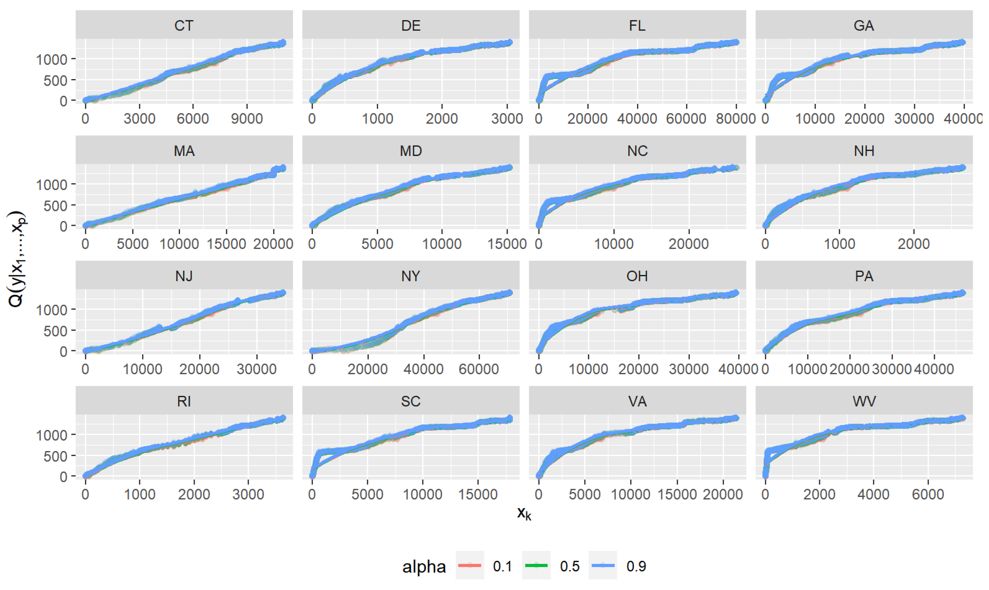
4.1. Graphical Visualization Using Copula

A copula is a multivariate distribution function defined by the unit [ 0 , 1 ] 2 with uniformly distributed marginals and describes the dependence mechanism between two random variables by eliminating the influence of the marginals or any monotone transformations of the marginals [3,4,11]. A bivariate distribution function, F ( y 1 , y 2 ) , can be represented as a function of its marginal distribution of Y 1 and Y 2 , F ( y 1 ) and F ( y 2 ) , by using a two-dimensional copula C ( · , · ) . More specifically, the copula may be written as
F ( y 1 , y 2 ) = C ( F ( y 1 ) , F ( y 2 ) ) = C ( u , v ) ,
where u and v are the continuous empirical marginal distribution functions F ( y 1 ) and F ( y 2 ) , respectively. Note that u and v have a uniform distribution U ( 0 , 1 ) .
Our study employs the Gaussian copula regression method to investigate the relationship between the state with the highest mortality and the rest of the states in the US. Let F ( · | x i ) be the marginal cumulative distribution for x i , then, the joint cumulative distribution function in the Gaussian copula regression can be expressed as
Pr ( Y 1 y 1 , , Y n y n ) = Φ n ϵ 1 , , ϵ n ; P ,
where ϵ i indicates a stochastic error that follows a multivariate standard normal distribution with a correlation matrix P. See [12] for more details.
Vine copulas were proposed by [13] to explain a multivariate dependence structure using copula due to the difficulty of expressing a multivariate joint distribution by copula [14,15,16]. Vine copulas are a graphical model that represent a d-dimensional multivariate density based on a pair-copula method given by [16] as follows:
f ( y ; ϕ ) = k = 1 d f k y k × i = 1 d 1 j = 1 d i c j , j + i ( j + 1 ) : ( j + i 1 ) F y j y j + 1 , , y j + i 1 , F y j + i y j + 1 , , y j + i 1 ; β j , j + i ( j + 1 ) : ( j + i 1 ) ,
where f k x k are the marginal densities, c j , j + i ( j + 1 ) : ( j + i 1 ) are the bivariate copula densities with parameter(s) β j , j + i ( j + 1 ) : ( j + i 1 ) , and ϕ is the set of all parameters in the D-vine density.
Figure 6 shows the marginal effects of a D-vine quantile regression model (10%, 50%, 90%) for the target variable DC with east coast states (CT, DE, FL, GA, MA, MD, NC, NH, NJ, NY, OH, PA, RI, SC, VA, WV) on the COVID-19 daily cumulative mortality data from 22 January 2020 to 1 September 2022. By using D-vine-based quantile regression with a selected copula out of all copula parametric and nonparametric families [18], we showed the linear and increasing marginal effects of each east coast state on Washington, D.C., as seen in Figure 6.
Figure 7 shows the R-vine copula [28]-based hierarchical tree dependence structure of five states’ (NY, CT, MA, NJ, DC) daily COVID-19 mortalities from 22 January 2020 to 1 September 2022 using the RVineStructureSelect command in the VineCopula R package. New York is located in the center among five east coast states and had relatively high Kendall’s tau correlations with CT (0.46), MA (0.47), NJ (0.46), and DC (0.44) in the level-one tree. This reminds us that New York City (NYC) was the early epicenter of the COVID-19 pandemic in the United States and affected neighboring states’ COVID-19 mortality numbers. In the level-two tree, NY had a 0.26 Kendall’s tau correlation with NJ and DC, a 0.27 Kendall’s tau correlation with DC and MA, and a 0.26 Kendall’s tau correlation with MA and CT. In the level-three tree, NY and MA had a 0.21 Kendall’s tau correlation with DC and CT and a 0.1 Kendall’s tau correlation with MA and NJ. In the level-four tree, CT and NJ had 0.14 Kendall’s tau correlation with NY, MA, and DC. We can see the conditional dependence relationships among five east coast states in Figure 7.

4.2. Gaussian Copula Marginal Regression

Since a traditional multiple linear regression is not appropriate for a non-normal and dispersed COVID-19 mortality data analysis, we applied the daily COVID-19 mortality data to the Gaussian copula marginal regression (GCMR) model using the gcmr R package. For our data analysis, GCMR models enable one to specify the correlation matrix of the errors. For this study, the correlation matrices of the autoregressive moving average (ARMA)(0,0), ARMA(0, 1), ARMA(1, 0), and ARMA(1, 1) were considered. To select the best GCMR model for the correlation matrix, four different GCMR models were compared with the Akaike information criterion (AIC). Before applying the GCMR models to the COVID-19 daily mortality data, we performed a stationary test using the augmented Dickey–Fuller statistic. Table 3 shows that the mortality data from the four big states (CA, TX, FL, NY) were stationary. We applied the GCMR models with a correlation matrix of ARMA(p,q), where p = 0 , 1 and q = 0 , 1 . Table 4 shows that the GCMR model that best fit the daily COVID-19 mortality data of CA was the GCMR model with a correlation matrix of ARMA(0,0), whereas the best fitting model for the daily COVID-19 mortality data of TX, FL, and NY was the GCMR model with a correlation matrix of ARMA(1,1). For the mortality data of CA, we found the following positively statistically significant states (AK 0.105, FL 0.249, GA 0.090, ID 0.070, NE 0.057, NY 0.072, TX 0.430, VT 0.071, WI 0.201) and the following negatively statistically significant states (HI −0.099, KY −0.091, MO −0.067, MT −0.083, OR −0.115, TN −0.108). Even though NY is far away from CA, there was a positive statistical effect on the mortality data of CA of 0.072. TX had the largest statistical effect on the mortality data of CA of 0.43. For the mortality data of TX, we found the following positively statistically significant states (AK 0.053, CA 0.273, CO 0.176, DC 0.050, FL 0.092, HI 0.051, MA 0.074, OH 0.077, WA 0.054) and the following negatively statistically significant states (AR −0.067, GA −0.067, IA −0.050, ID −0.049, MN −0.085). CA had the largest statistical effect on the mortality data of TX of 0.273. For the mortality data of FL, we found the following positively statistically significant states (CA 0.391, DC 0.069, HI 0.106, LA 0.078, NC 0.130, OH 0.225, TX 0.188) and the following negatively statistically significant states (AZ −0.075, NY −0.089). It is interesting to see that NY had a negative statistically significant effect on the mortality data of FL. CA had the largest statistical effect on the mortality data of FL of 0.391. For the mortality data of NY, we found the following positively statistically significant states (AR 0.169, CA 0.063, DC 0.069, HI 0.062, IN 0.094, MA 0.116, NM 0.130, UT 0.094, WV 0.139, WY 0.073) and the following negatively statistically significant states (GA −0.095, MT −0.086, PA −0.079). PA had a negative statistically significant effect on the mortality data of NY despite PA being a neighboring state of NY.

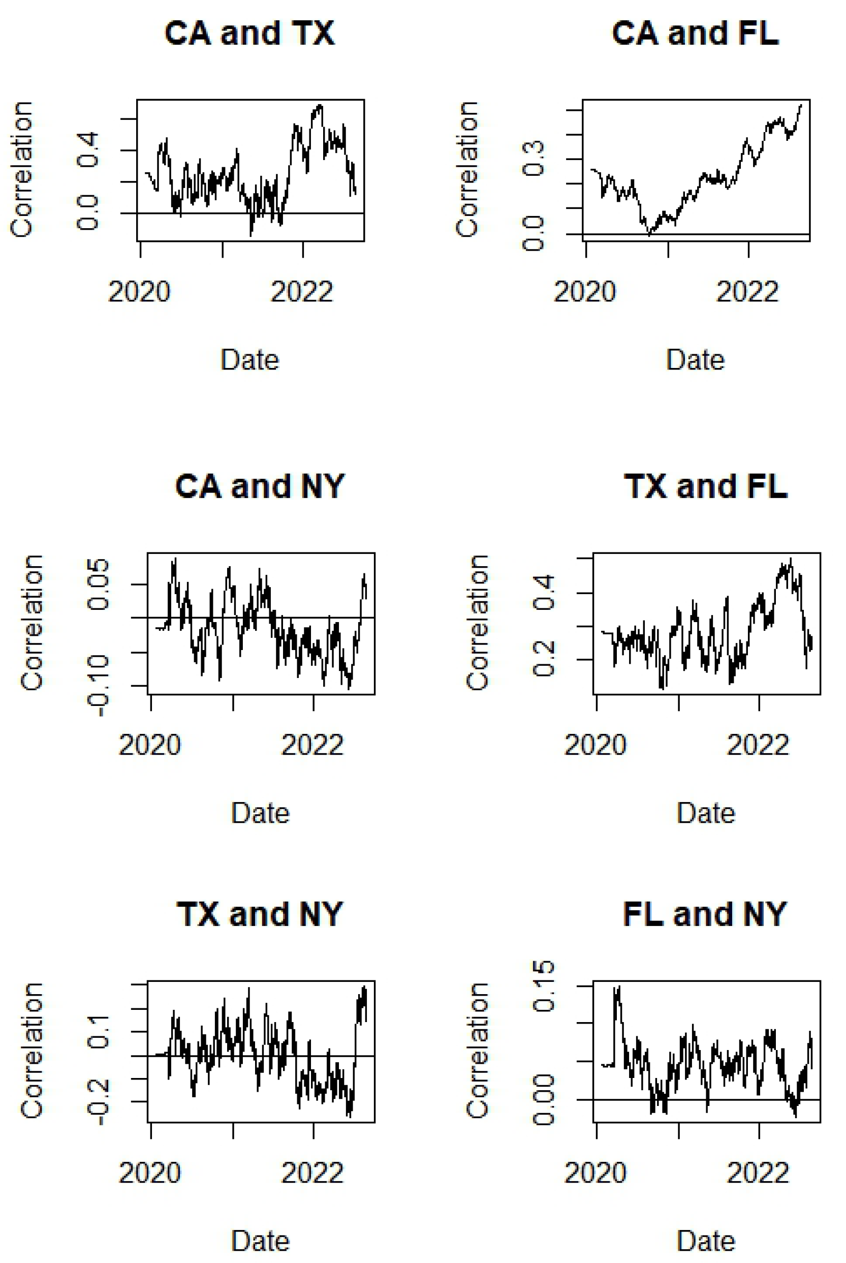
4.3. Copula Dynamic Conditional Correlation

The copula dynamic conditional correlation (Copula-DCC) is an extension of the DCC model. The time-varying conditional correlation in the copula framework was developed by [29].
Let r t = ( r i t , , r n t ) be an n × 1 vector of the daily COVID-19 mortality data and it follows a copula GARCH model with joint distribution given by
F ( r t | μ t , h t ) = C ( F 1 ( r 1 t | μ 1 t , h 1 t ) , , F n ( r n t | μ n t , h n t ) )
where F i and C are the conditional distribution and the copula function, respectively.
It is formulated that the conditional mean E [ r i t | t 1 ] = μ i t is a linear function of its one-lag past the mortality data and follows an ARMA(1,1) process. The conditional variance h i t is assumed to follow a gjr-GARCH(1,1) process. One can thus consider
r i t = μ i t + θ 1 ( r i t 1 μ i t ) + θ 2 ϵ i t 1 2 + ϵ i t , ϵ i t = h i t z i t
h i t 2 = ω + α 1 ε i t 1 2 + γ 1 I i t 1 ε i t 1 2 + β 1 h i t 1
where h i t 2 is the conditional variance and ω is the intercept. Further, β 1 and α 1 are the ARCH and GARCH terms, γ 1 denotes the leverage term, the indicator function I takes values one and zero according to the “bad” news ( negative   shock , ε i t 1 < 0 ) and the “good” news ( positive   shock , ε i t 1 0 ) , respectively. Note that the coefficients α 1 + γ 1 and α 1 correspond, respectively, to the “bad" news and “good" news. When γ 1 > 0 , the negative shock produces a greater response than the positive shock. Here, z i t are i.i.d. random variables, which follow Johnson’s reparametrized SU distribution, viz., z i t J S U ( μ , σ , ν , τ ) in [30], where the four parameters ( μ , σ , ν , τ ) are the mean, standard deviation, skew, and shape parameters, respectively. The dependence structure is modeled using elliptical copulas with conditional correlation R t and constant shape parameter τ . The conditional density with a Gaussian copula is given by (see, for instance, reference [4])
c t ( u i t , , u n t | R t ) = f t F i 1 ( u i t ) , , F i 1 ( u n t ) | R t i = 1 n f i F i 1 ( u i t )
where u i t = F i t ( r i t | μ i t , h i t , ν t , τ i ) is the probability integral transformed values by F i t , which can be obtained using the gjr GARCH process, and F i 1 ( u i t | τ ) represents the quantile transformation. The Gaussian copula conditional correlation can be obtained using the function cgarchspec command in the R package rmgarch.
Table 5 shows that the mean equation error structure followed ARMA(1,1) for the daily COVID-19 mortality data of CA, TX, FL, and NY, and the coefficients on the AR 1 and MA 1 terms were statistically significant in CA, TX, FL, and NY. The estimates of γ 1 s in the variance equations in CA and NY were statistically significant at the 1% significance level. This means that the negative shock produced a greater response than the positive shock in terms of the daily COVID-19 mortality data in CA and NY. The estimates of α 1 s in the variance equations in TX and FL were statistically significant at the 1% significance level. This means that the positive shock produced a greater response than the negative shock in terms of the daily COVID-19 mortality data in TX and FL.
Figure 8 shows the two-state plots of the copula-DCC model for CA, TX, FL, and NY. In Figure 8, the estimated time-varying conditional correlations of the daily COVID-19 mortality data for CA and FL had increased over the previous two years and the estimated time-varying conditional correlations of the daily COVID-19 mortality data for CA and TX and TX and FL had decreased rapidly over the 2022 summer period by 1 September 2022. Another interesting finding from Figure 8 is that the time-varying correlation of the daily COVID-19 mortality data for CA and NY over the given period varied between −0.10 and 0.10. The geographical distance between CA (west coast) and NY (east coast) is about 2900 miles, which can make the time-varying correlations of the daily COVID-19 mortality data for CA and NY become smaller.

5. Discussion

We used the graphical models FPCA, GCMR, vine copula-based quantile regression, and copula-DCC for visual and data analysis of the COVID-19 mortality data in the 50 US states plus Washington, D.C., from the beginning of the COVID-19 pandemic to 1 September 2022 because the COVID-19 mortality data have a non-normal distribution and non-constant variance in the errors. Looking at the results of the graphical model, we found five equivalence groups in the US. Looking at the results of the FPCA, we visualized the COVID-19 daily mortality time trends of 50 states plus Washington, D.C. Using the GCMR model, we investigated the COVID-19 daily mortality relationships between four major states and the rest of the states in the US. Using the copula-DCC models, we investigated the time-varying dependence relationships between the COVID-19 daily mortality data of four major states (CA, TX, FL, and NY). Based on the findings of this research, geographical distance can be considered one of the main factors in the exponential increase in the number of pandemic patients from one state to the neighboring states in a short period of time. When a pandemic or an endemic happens in a certain state, the local state government needs to cooperate with federal and neighboring state governments to take immediate public health emergency measures. Time is one of the most important factors in suppressing a pandemic or endemic so we emphasize the need for a timely public health emergency response when facing a pandemic such as COVID-19. Every state in the US needs to regularly check its public health emergency manuals to prepare for future pandemics or natural disasters. In our future study, we will consider visualizing international COVID-19 mortality time-course pattern clustering by functional principal component analysis so that we can help to quickly control future pandemics.

Funding

This research received no external funding.

Data Availability Statement

Not applicable.

Acknowledgments

The author thanks the respected editor and the two respected anonymous referees for the constructive and helpful suggestions that led to substantial improvements in the revised version and also thanks Grace Kim (Wayzata High School Student, MN) for her COVID-19 data collection help and discussion of this research topic.

Conflicts of Interest

The author declares no conflict of interest.

References

  1. Ramsay, J.; Silverman, B. Functional Data Analysis, 2nd ed.; Springer: New York, NY, USA, 2005. [Google Scholar]
  2. Kokoszka, P.; Reimherr, M. Introduction to Functional Data Analysis, 1st ed.; Chapman and Hall/CRC: Boca Raton, FL, USA, 2017. [Google Scholar]
  3. Joe, H. Multivariate Models and Multivariate Dependence Concepts; CRC Press: Boca Raton, FL, USA, 1997. [Google Scholar]
  4. Nelsen, R.B. An Introduction to Copulas, 2nd ed.; Springer Science & Business Media: Berlin/Heidelberg, Germany, 2013. [Google Scholar]
  5. Tang, C.; Wang, T.; Zhang, P. Functional Data Analysis: An Application to COVID-19 Data in the United States. arXiv 2020. [Google Scholar] [CrossRef]
  6. Lia, X.; Zhang, P.; Feng, Q. Exploring COVID-19 in mainland China during the lockdown of Wuhan via functional data analysis. Commun. Stat. Methods 2022, 29, 103–125. [Google Scholar]
  7. Oshinubi, K.; Ibrahim, F.; Rachdi, M.; Demongeot, J. Functional data analysis: Application to daily observation of COVID-19 prevalence in France. AIMS Math. 2022, 7, 5347–5385. [Google Scholar] [CrossRef]
  8. Acal, C.; Escabias, M.; Aguilera, A.M.; Valderrama, M.J. COVID-19 Data Imputation by Multiple Function-on-Function Principal Component Regression. Mathematics 2021, 9, 1237. [Google Scholar] [CrossRef]
  9. Cherubini, U.; Luciano, E.; Vecchiato, W. Copula Methods in Finance; John Wiley: Chichester, UK, 2004. [Google Scholar]
  10. Kim, J.-M. A Review of Copula Methods for Measuring Uncertainty in Finance and Economics. Quant. Bio-Sci. 2020, 39, 81–90. [Google Scholar]
  11. Sklar, A. Fonctions de repartition á n dimensions et leurs marges. Publ. Inst. Statist. Univ. Paris 1959, 8, 229–231. [Google Scholar]
  12. Masarotto, G.; Varin, C. Gaussian copula marginal regression. Electron. J. Stat. 2020, 6, 1517–1549. [Google Scholar] [CrossRef]
  13. Joe, H. Families of m-variate distributions with given margins and m(m−1)/2 bivariate dependence parameters. In Distributions with Fixed Marginals and Related Topics; Rüschendorf, L., Schweizer, B., Taylor, M.D., Eds.; Lecture Notes—Monograph Series; Institute of Mathematical Statistics: Tokyo, Japan, 1996; pp. 120–141. [Google Scholar] [CrossRef]
  14. Bedford, T.; Cooke, R.M. Vines—A new graphical model for dependent random variables. Ann. Stat. 2002, 30, 1031–1068. [Google Scholar] [CrossRef]
  15. Aas, K.; Berg, D. Models for construction of multivariate dependence: A comparison study. Eur. Financ. 2009, 15, 639–659. [Google Scholar] [CrossRef]
  16. Aas, K.; Czado, C.; Frigessi, A.; Bakken, H. Pair-copula constructions of multiple dependence. Insur. Math. Econ. 2009, 44, 182–198. [Google Scholar] [CrossRef] [Green Version]
  17. Brechmann, E.C.; Schepsmeier, U. Modeling Dependence with C- and D-Vine Copulas: The R Package CDVine. J. Stat. Softw. 2013, 52, 1–27. [Google Scholar] [CrossRef] [Green Version]
  18. Kraus, D.; Czado, C. D-vine copula based quantile regression. Comput. Stat. Data Anal. 2017, 110, 1–18. [Google Scholar] [CrossRef]
  19. D’Urso, P.; De Giovanni, L.; Vitale, V. A D-Vine Copula-Based Quantile Regression Model with Spatial Dependence for COVID-19 Infection Rate in Italy. Spat. Stat. 2022, 47, 100586. [Google Scholar] [CrossRef] [PubMed]
  20. Taamouti, A.; Doukali, M.; Bouezmarni, T. Copula-Based Estimation of Health Concentration Curves with an Application to COVID-19. Available online: https://ssrn.com/abstract=4064991 (accessed on 15 August 2022).
  21. Ansell, L.; Valle, L.D. A New Data Integration Framework for Covid-19 Social Media Information. arXiv 2021. [Google Scholar] [CrossRef]
  22. Kalisch, M.; Hauser, A.; Maathuis, M.H.; Mächler, M. An Overview of the pcalg Package for R; CRAN of R Project: Vienna, Austria, 2019; Available online: https://cran.microsoft.com/snapshot/2019-08-16/web/packages/pcalg/vignettes/vignette2018.pdf (accessed on 15 August 2022).
  23. Wang, J.-L.; Chiou, J.-M.; Muüller, H.-G. Functional Data Analysis. Annu. Rev. Stat. Appl. 2016, 3, 257–295. [Google Scholar] [CrossRef] [Green Version]
  24. Chen, K.; Zhang, X.; Petersen, A.; Muüller, H.-G. Quantifying Infinite-Dimensional Data: Functional Data Analysis in Action. Stat. Biosci. 2017, 9, 582–604. [Google Scholar] [CrossRef]
  25. Pearson, K.F.R.S. LIII. On lines and planes of closest fit to systems of points in space. Lond. Edinb. Dublin Philos. Mag. J. Sci. 1901, 2, 559–572. [Google Scholar] [CrossRef] [Green Version]
  26. Ramsay, J.O.; Hooker, G.; Graves, S. Functional Data Analysis with R and MATLAB; Springer Science & Business Media: New York, NY, USA, 2009. [Google Scholar]
  27. Craven, P.; Wahba, G. Smoothing Noisy Data with Spline Functions. Estimating the Correct Degree of Smoothing by the Method of Generalized CrossValidation. Numer. Math. 1979, 31, 377–403. [Google Scholar] [CrossRef]
  28. Dissmann, J.F.; Brechmann, E.C.; Czado, C.; Kurowicka, D. Selecting and estimating regular vine copulae and application to financial returns. Comput. Stat. Data Anal. 2013, 59, 52–69. [Google Scholar] [CrossRef] [Green Version]
  29. Kim, J.-M.; Jung, H. Linear Time Varying Regression with Copula DCC-GARCH Model for Volatility. Econ. Lett. 2016, 145, 262–265. [Google Scholar] [CrossRef]
  30. Ghalanos, A. The Rmgarch Models: Background and Properties. (Version 1.3-0). 2019. Available online: https://cran.microsoft.com/snapshot/2020-05-24/web/packages/rmgarch/vignettes/The_rmgarch_models.pdf (accessed on 15 August 2022).
Figure 1. COVID-19 daily cumulative mortality data for 50 states and Washington, D.C. (22 January 2020 to 1 September 2022).
Axioms 11 00619 g001
Figure 2. Estimated CPDAG with COVID-19 daily cumulative mortality data from 50 states and Washington, D.C. (22 January 2020 to 1 September 2022).
Axioms 11 00619 g002
Figure 3. 2D Plot of FPCA for Daily COVID-19 Mortality Data.
Axioms 11 00619 g003
Figure 4. 3D Plot of FPCA for Daily COVID-19 Mortality Data.
Axioms 11 00619 g004
Figure 5. Plots of linear regression for NY with CA, TX, FL cumulative daily COVID-19 mortality data (22 January 2020 to 1 September 2022).
Axioms 11 00619 g005
Figure 6. Plots of marginal effects of a D-vine quantile regression model (10%, 50%, 90%) for DC on the COVID-19 daily cumulative mortality data for CT, DE, FL, GA, MA, MD, NC, NH, NJ, NY, OH, PA, RI, SC, VA, WV (22 January 2020 to 1 September 2022).
Axioms 11 00619 g006
Figure 7. R-vine copula model-based hierarchical tree structure plots of daily COVID-19 mortality data (22 January 2020 to 1 September 2022).
Axioms 11 00619 g007
Figure 8. Plots of copula-DCC model for CA, TX, FL, and NY.
Axioms 11 00619 g008
Table 1. Summary Statistics for US Daily COVID-19 Mortalities and 2022 US State Populations.
AKALARAZCACOCTDCDEFLGAHIIAIDILINKS
Mean1.321.212.531.398.613.811.61.53.28441.71.710.45.44025.79.4
Median0766546100442500122130
SD5.23919.558.1142.225.323.32.97.6152.292.84.129.19.653.158.727.4
Kurtosis8721.470.614.1636.213.556.5104.629.2516.844.41089.76.5471.844.6
Skewness8.53.95.83.32.44.83.25.47.94.719.758.12.82.318.65.5
Minimum00000000000000000
Maximum68389322498704309204451331552249959518654011546371
Total128120,16011,92329,85293,92413,14811,0341382304280,02739,77216449940511538,16124,4548958
Count953953953953953953953953953953953953953953953953953
Population738,0235,073,1873,030,6467,303,39839,995,0775,922,6183,612,314644,7431,008,35022,085,56310,916,7601,474,2653,219,1711,893,41012,808,8846,845,8742,954,832
Mortality Rate0.17%0.40%0.39%0.41%0.23%0.22%0.31%0.21%0.30%0.36%0.36%0.11%0.31%0.27%0.30%0.36%0.30%
KYLAMAMDMEMIMNMOMSMTNCNDNENHNJNMNV
Mean17.518.822.115.92.639.913.42113.43.727.62.34.72.836.38.912
Median61010917736111001953
SD33.727.33729671.918.8104206.956.46.515.65108.610.721.6
Kurtosis44.640.526.3159.548.610.76.2603.59.614.2186.9220.7433.724.12137.482.2
Skewness5.44.63.910.15.62.92.322.32.63.310.511.617.83.912.72.16.4
Minimum00000000000000000
Maximum44836245954983566140288117755117214039959203799365
Total16,67917,87721,03515,199251238,03812,80619,99312,794350426,33522324455266234,567846511,400
Count953953953953953953953953953953953953953953953953953
Population4,539,1304,682,6337,126,3756,257,9581,369,15910,116,0695,787,0086,188,1112,960,0751,103,18710,620,168800,3941,988,5361,389,7419,388,4142,129,1903,185,426
Mortality Rate0.37%0.38%0.30%0.24%0.18%0.38%0.22%0.32%0.43%0.32%0.25%0.28%0.22%0.19%0.37%0.40%0.36%
NYOHOKORPARISCSDTNTXUTVAVTWAWIWVWY
Mean74.441.417.58.8493.818.83.128.892.95.222.50.714.715.87.72
Median230032207084521106620
SD149.712566.914.169.912.130.58.490.6103.57.638.41.524.12514.57.7
Kurtosis23.9185.42613.67.153.112.119.2338.92.57.634.117.519.81134.339.2
Skewness4.410.94.932.36.63415.61.42.34.93.33.52.94.65.7
Minimum00000000000000000
Maximum14602559548134547137241782174798654041625620617081
Total70,87739,49016,720841546,716364517,869299327,48788,578498121,43970714,03915,08472911881
Count953953953953953953953953953953953953953953953953953
Population20,365,87911,852,0364,000,9534,318,49213,062,7641,106,3415,217,037901,1657,023,78829,945,4933,373,1628,757,467646,5457,901,4295,935,0641,781,860579,495
Mortality Rate0.35%0.33%0.42%0.19%0.36%0.33%0.34%0.33%0.39%0.30%0.15%0.24%0.11%0.18%0.25%0.41%0.32%
Table 2. Total Cumulative Percentage Variations in the Daily COVID-19 Mortality Data of Five Functional Principal Components for Daily COVID-19 Mortality Data.
FPC1FPC2FPC3FPC4FPC5
PV0.81940.11250.05120.01170.0052
CPV0.81940.93200.98310.99481.0000
Table 3. Stationary Test Using Augmented Dickey–Fuller Statistic.
CATXFLNY
Dickey–Fuller Statistic−18.02−12.118−21.365−15.552
p-value0.010.010.010.01
StationaryYesYesYesYes
Table 4. GCMR results.
CAEstimateStd. Errorz valuep-ValueTXEstimateStd. Errorz Valuep-ValueFLEstimateStd. Errorz Valuep-ValueNYEstimateStd. Errorz Valuep-Value
Intercept0.0070.0360.2100.834Intercept0.3340.0774.3550.000Intercept−0.0190.065−0.2920.770Intercept0.0300.0550.5420.588
AK0.1050.0283.8130.000AK0.0530.0212.5050.012AK0.0000.0320.0140.989AK−0.0320.024−1.3590.174
AL−0.0260.030−0.8650.387AL0.0240.0231.0310.303AL0.0090.0340.2620.793AL−0.0360.026−1.4240.154
AR−0.0120.035−0.3550.723AR−0.0670.029−2.3380.019AR−0.0710.042−1.6830.092AR0.1690.0325.3160.000
AZ0.0540.0321.6860.092AZ0.0220.0250.8660.386AZ−0.0750.037−2.0130.044AZ0.0410.0281.4520.146
CO−0.0080.024−0.3170.752CA0.2730.02511.0320.000CA0.3910.03710.6210.000CA0.0630.0292.1610.031
CT−0.0340.034−0.9990.318CO0.1760.0199.3210.000CO0.0160.0290.5490.583CO−0.0230.022−1.0410.298
DC0.0010.0290.0220.982CT−0.0040.025−0.1580.874CT0.0260.0380.6860.493CT0.0110.0280.3770.706
DE0.0630.0272.3830.017DC0.0500.0222.2650.024DC0.0690.0332.0880.037DC0.0690.0252.7640.006
FL0.2490.0269.7180.000DE−0.0170.020−0.8790.380DE−0.0450.029−1.5340.125DE0.0430.0221.9510.051
GA0.0900.0342.6550.008FL0.0920.0224.2600.000GA−0.0120.039−0.3180.751FL−0.0470.024−1.9390.053
HI−0.0990.031−3.2130.001GA−0.0670.026−2.5660.010HI0.1060.0353.0230.003GA−0.0950.029−3.2710.001
IA0.0300.0281.0420.297HI0.0510.0242.1740.030IA0.0180.0330.5440.586HI0.0620.0262.3530.019
ID0.0700.0302.3140.021IA−0.0500.022−2.2900.022ID−0.0190.034−0.5510.581IA−0.0040.024−0.1840.854
IL−0.0150.041−0.3610.718ID−0.0490.023−2.1560.031IL0.0520.0491.0590.289ID−0.0260.026−1.0140.310
IN0.0690.0401.6980.089IL−0.0220.033−0.6790.497IN0.0130.0470.2800.780IL0.0110.0360.3030.762
KS0.0030.0280.1130.910IN−0.0060.032−0.1990.842KS0.0100.0310.3160.752IN0.0940.0352.6530.008
KY−0.0910.033−2.7090.007KS−0.0180.020−0.8810.378KY0.0410.0401.0140.311KS0.0190.0230.8310.406
LA−0.0010.030−0.0390.969KY0.0200.0270.7520.452LA0.0780.0372.1050.035KY0.0520.0301.7460.081
MA0.0140.0310.4620.644LA0.0000.025−0.0140.989MA−0.0670.042−1.5920.111LA0.0380.0281.3520.176
MD0.0570.0291.9520.051MA0.0740.0292.5740.010MD0.0620.0361.7300.084MA0.1160.0323.5960.000
ME−0.0290.025−1.1370.255MD0.0460.0241.9140.056ME−0.0130.029−0.4520.651MD0.0150.0270.5490.583
MI0.0250.0300.8160.415ME−0.0280.020−1.4170.157MI0.0590.0341.7240.085ME−0.0500.022−2.2850.022
MN−0.0360.036−0.9870.324MI−0.0260.023−1.1390.255MN0.0810.0431.8900.059MI−0.0170.025−0.6660.506
MO−0.0670.030−2.2030.028MN−0.0850.029−2.9580.003MO0.0580.0341.7090.087MN0.0400.0321.2320.218
MS0.0250.0350.7200.472MO−0.0100.023−0.4320.666MS−0.0240.040−0.6020.547MO−0.0050.026−0.1880.851
MT−0.0830.032−2.5450.011MS−0.0120.027−0.4400.660MT0.0490.0371.3190.187MS−0.0240.030−0.8110.417
NC−0.0020.036−0.0540.957MT−0.0030.025−0.1110.911NC0.1300.0413.1440.002MT−0.0860.028−3.0650.002
ND−0.0310.027−1.1730.241NC0.0110.0280.3940.694ND−0.0280.031−0.8950.371NC0.0420.0311.3420.180
NE0.0570.0272.1020.036ND−0.0050.021−0.2250.822NE−0.0580.031−1.9020.057ND−0.0320.023−1.3550.175
NH0.0160.0280.5740.566NE−0.0180.021−0.8900.374NH−0.0010.032−0.0410.967NE−0.0230.023−1.0150.310
NJ0.0410.0301.3630.173NH−0.0060.021−0.2740.784NJ0.0170.0440.3930.695NH0.0090.0240.3660.714
NM0.0520.0351.4590.145NJ0.0140.0310.4440.657NM−0.0590.044−1.3550.175NJ0.0610.0351.7700.077
NV0.0140.0330.4280.668NM0.0450.0301.5200.128NV−0.0020.036−0.0620.950NM0.1300.0333.9620.000
NY0.0720.0352.0650.039NV−0.0360.024−1.5110.131NY−0.0890.043−2.0890.037NV−0.0340.027−1.2750.202
OH−0.0380.029−1.2790.201NY−0.0380.029−1.3050.192OH0.2250.0336.7990.000OH0.0010.0250.0570.954
OK0.0060.0360.1650.869OH0.0770.0233.4350.001OK−0.0450.042−1.0750.282OK0.0140.0310.4550.649
OR−0.1150.033−3.4540.001OK−0.0550.028−1.9960.046OR0.0340.0380.8900.374OR0.0250.0280.8820.378
PA−0.0190.031−0.6030.546OR−0.0160.025−0.6500.515PA−0.0350.037−0.9590.338PA−0.0790.027−2.9130.004
RI0.0070.0270.2560.798PA−0.0210.025−0.8720.383RI−0.0150.032−0.4690.639RI0.0270.0241.1310.258
SC0.0470.0341.3840.166RI−0.0150.021−0.7150.475SC0.0590.0381.5430.123SC0.0050.0290.1840.854
SD−0.0220.030−0.7400.459SC−0.0310.026−1.2210.222SD0.0170.0340.4900.624SD0.0070.0250.2600.795
TN−0.1080.029−3.6840.000SD−0.0430.022−1.9220.055TN−0.0330.035−0.9250.355TN−0.0050.026−0.1940.846
TX0.4300.03014.2380.000TN0.0160.0230.6670.505TX0.1880.0464.1070.000TX−0.0530.036−1.4940.135
UT−0.0230.032−0.7260.468UT−0.0110.024−0.4630.644UT−0.0180.036−0.5040.615UT0.0940.0273.5130.000
VA0.0380.0291.2840.199VA0.0020.0240.0680.946VA0.0450.0351.2920.196VA0.0920.0263.4930.000
VT0.0710.0272.6910.007VT0.0050.0210.2300.818VT−0.0420.031−1.3420.179VT−0.0030.023−0.1330.894
WA−0.0280.027−1.0510.293WA0.0540.0202.6760.007WA0.0470.0301.5540.120WA0.0420.0231.8390.066
WI0.2010.0277.4660.000WI0.0300.0221.3860.166WI−0.0030.033−0.1050.917WI0.0100.0240.4060.685
WV−0.0050.031−0.1650.869WV−0.0190.025−0.7840.433WV−0.0620.037−1.6970.090WV0.1390.0275.0720.000
WY−0.0310.035−0.8770.381WY0.0000.0250.0010.999WY−0.0300.038−0.7950.427WY0.0730.0282.5820.010
sigma0.1640.00443.6670.000sigma0.2020.01910.8320.000sigma0.2140.01415.1390.000sigma0.1820.01611.4410.000
A R 1 0.9890.003317.6000.000 A R 1 0.9830.007137.5100.000 A R 1 0.9790.008124.0100.000
M A 1 −0.8060.018−45.9700.000 M A 1 −0.8750.016−53.2100.000 M A 1 −0.8070.023−34.9500.000
Table 5. Copula-DCC Models.
CA and TXTX and FL
CAEstimateStd. Errorz valuep-valueTXEstimateStd. Errorz valuep-valueTXEstimateStd. Errorz valuep-valueFLEstimateStd. Errorz valuep-value
μ 0.100.026.350.00 μ 0.080.0034.660.00 μ 0.080.0034.730.00 μ 0.100.019.470.00
AR 1 1.000.00816.060.00 AR 1 1.000.01157.530.00 AR 1 1.000.01157.680.00 AR 1 1.000.0255.000.00
MA 1 −0.640.02−26.300.00 MA 1 −0.500.11−4.670.00 MA 1 −0.500.11−4.670.00 MA 1 −0.780.23−3.400.00
ω 0.000.001.040.30 ω 0.000.000.001.00 ω 0.000.000.001.00 ω 0.000.000.001.00
α 1 0.130.034.720.00 α 1 0.460.232.010.04 α 1 0.460.232.010.04 α 1 0.450.172.680.01
β 1 0.830.0328.650.00 β 1 0.520.153.580.00 β 1 0.520.153.580.00 β 1 0.470.123.880.00
γ 1 0.090.042.240.03 γ 1 0.030.190.170.87 γ 1 0.030.190.170.87 γ 1 0.160.161.020.31
skew1.550.542.860.00skew−0.050.08−0.660.51skew−0.050.08−0.660.51skew0.200.430.470.64
shape3.010.624.860.00shape1.240.177.320.00shape1.240.177.320.00shape1.240.264.820.00
[Joint]dcca10.040.012.670.01Log−Likelihood2215.84AIC−4.61 [Joint]dcca10.020.020.870.38Log−Likelihood1549.04AIC−3.21
[Joint]dccb10.940.0243.260.00N953BIC−4.51 [Joint]dccb10.960.0616.160.00N953BIC−3.11
CA and FLTX and NY
CAEstimateStd. Errorz valuep-valueFLEstimateStd. Errorz valuep-valueTXEstimateStd. Errorz valuep-valueNYEstimateStd. Errorz valuep-value
μ 0.100.026.350.00 μ 0.100.019.470.00 μ 0.080.0034.690.00 μ 0.120.00679.520.00
AR 1 1.000.00815.720.00 AR 1 1.000.0254.940.00 AR 1 1.000.01157.550.00 AR 1 1.000.00367.850.00
MA 1 −0.640.02−26.340.00 MA 1 −0.780.23−3.400.00 MA 1 −0.500.11−4.670.00 MA 1 −0.730.08−9.130.00
ω 0.000.001.040.30 ω 0.000.000.001.00 ω 0.000.000.001.00 ω 0.000.000.001.00
α 1 0.130.034.730.00 α 1 0.450.172.680.01 α 1 0.460.232.010.04 α 1 0.350.142.480.01
β 1 0.830.0328.710.00 β 1 0.470.123.890.00 β 1 0.520.153.580.00 β 1 0.490.076.690.00
γ 1 0.090.042.240.03 γ 1 0.160.161.020.31 γ 1 0.030.190.170.87 γ 1 0.320.171.940.05
skew1.550.542.860.00skew0.200.430.470.64skew−0.050.08−0.660.51skew−0.370.19−1.930.05
shape3.010.624.860.00shape1.240.264.830.00shape1.240.177.320.00shape1.150.186.550.00
[Joint]dcca10.010.003.000.00Log−Likelihood1293.03AIC−2.67 [Joint]dcca10.030.012.900.00Log−Likelihood1814.15AIC−3.77
[Joint]dccb10.990.00253.890.00N953BIC−2.57 [Joint]dccb10.920.0330.720.00N953BIC−3.66
CA and NYFL and NY
CAEstimateStd. Errorz valuep-valueNYEstimateStd. Errorz valuep-valueFLEstimateStd. Errorz valuep-valueNYEstimateStd. Errorz valuep-value
μ 0.100.026.350.00 μ 0.110.00678.780.00 μ 0.100.019.460.00 μ 0.120.00679.310.00
AR 1 1.000.00816.340.00 AR 1 1.000.00366.630.00 AR 1 1.000.0254.910.00 AR 1 1.000.00367.740.00
MA 1 −0.640.03−26.190.00 MA 1 −0.730.08−9.110.00 MA 1 −0.780.23−3.400.00 MA 1 −0.730.08−9.130.00
ω 0.000.001.040.30 ω 0.000.000.001.00 ω 0.000.000.001.00 ω 0.000.000.001.00
α 1 0.130.034.720.00 α 1 0.350.142.480.01 α 1 0.450.172.680.01 α 1 0.350.142.480.01
β 1 0.830.0328.670.00 β 1 0.490.076.690.00 β 1 0.470.123.880.00 β 1 0.490.076.690.00
γ 1 0.090.042.240.03 γ 1 0.320.171.930.05 γ 1 0.160.161.020.31 γ 1 0.320.171.930.05
skew1.550.542.860.00skew−0.370.19−1.930.05skew0.200.430.470.64skew−0.370.19−1.930.05
shape3.010.624.850.00shape1.150.186.550.00shape1.240.264.820.00shape1.150.186.550.00
[Joint]dcca10.010.011.280.20Log−Likelihood1545.17AIC−3.20 [Joint]dcca10.010.011.300.19Log−Likelihood892.30AIC−1.83
[Joint]dccb10.960.0424.010.00N953BIC−3.10 [Joint]dccb10.950.0240.340.00N953BIC−1.73
Publisher’s Note: MDPI stays neutral with regard to jurisdictional claims in published maps and institutional affiliations.

