
Evaluating Global Container Shipping Companies: A Novel Approach to Investigating Both Qualitative and Quantitative Criteria for Sustainable Development

 ,
,  ,
,  , and
, and 
Abstract
:1. Introduction
1.1. Research Background
1.2. CSCs’ Efficiency Measurements
1.3. Objectives of Present Study
2. Literature Review
2.1. Literature Review on Efficiency Analysis of CSCs
2.2. Research Gaps
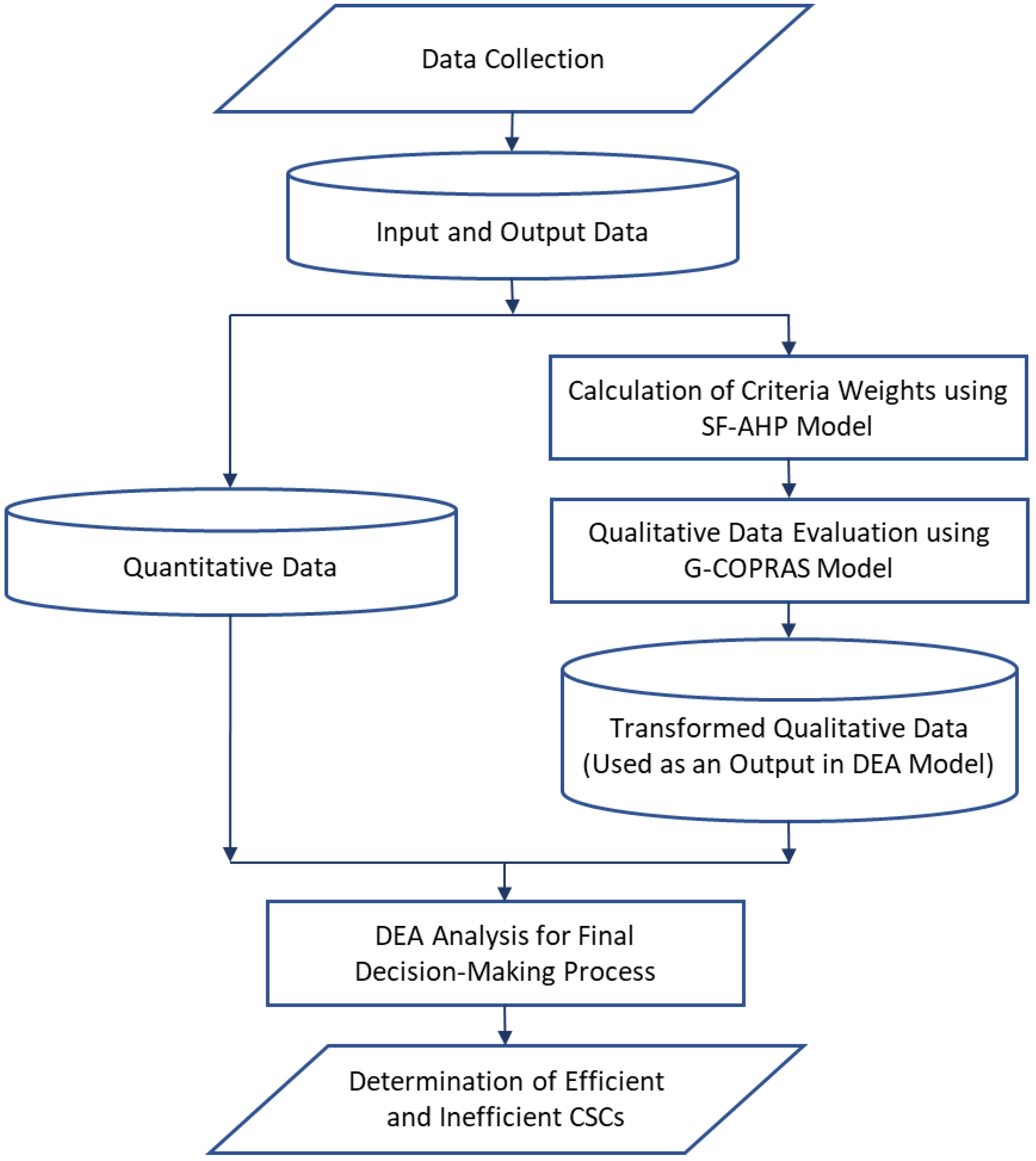
3. Methodology
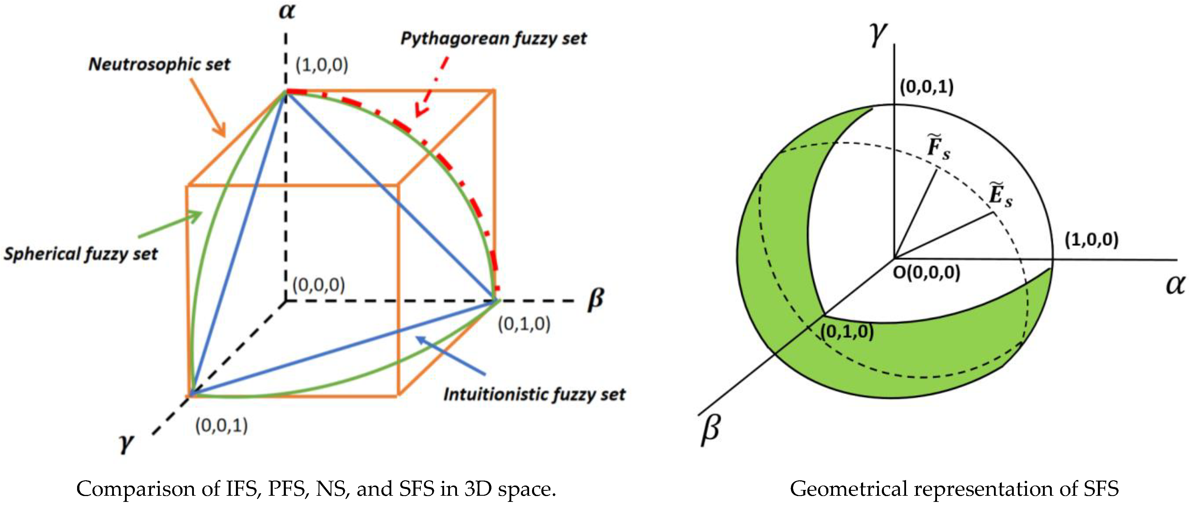
3.1. Spherical Fuzzy Analytical Hierarchy Process (AHP-SF)
- Union operation
- Intersection operation
- Addition operation
- Multiplication operation
- Multiplication by a scalar;
- Power of
3.2. Grey Complex Proportional Assessment (COPRAS-G)
3.3. Data Envelopment Analysis (DEA)
- : number of decision-making units (DMUs), as shipping companies in this paper
- : the DMU, , has inputs, desirable outputs, undesirable outputs
- : the input of the DMU, the matrix as
- : the desirable output, the matrix as
- : the undesirable output, the matrix as
- : the model adjusts the desirable output by the negative impact of shipping emissions (i.e., undesirable output model)
- : otherwise
4. Empirical Analysis
4.1. Phase 1: Qualitative Efficiency Analysis
4.1.1. The Use of AHP-SF for Determination Criteria Weights and Results
4.1.2. The Use of COPRAS-G and Results
4.2. Phase 2: Finding the Ranking of Efficient and Inefficient CSCs with DEA and Final Results
5. Discussions and Conclusions
Author Contributions
Funding
Data Availability Statement
Acknowledgments
Conflicts of Interest
Appendix A

| Criteria | C1 | C2 | C3 | SE1 | SE2 | ||||||||||
|---|---|---|---|---|---|---|---|---|---|---|---|---|---|---|---|
| C1 | 0.500 | 0.400 | 0.400 | 0.569 | 0.412 | 0.311 | 0.495 | 0.468 | 0.349 | 0.535 | 0.454 | 0.310 | 0.562 | 0.412 | 0.319 |
| C2 | 0.381 | 0.603 | 0.296 | 0.500 | 0.400 | 0.400 | 0.485 | 0.498 | 0.314 | 0.485 | 0.502 | 0.311 | 0.557 | 0.415 | 0.321 |
| C3 | 0.446 | 0.509 | 0.352 | 0.450 | 0.525 | 0.297 | 0.500 | 0.400 | 0.400 | 0.423 | 0.564 | 0.307 | 0.382 | 0.617 | 0.268 |
| SE1 | 0.421 | 0.567 | 0.303 | 0.459 | 0.522 | 0.061 | 0.526 | 0.449 | 0.321 | 0.500 | 0.400 | 0.400 | 0.404 | 0.583 | 0.300 |
| SE2 | 0.381 | 0.597 | 0.303 | 0.391 | 0.584 | 0.187 | 0.429 | 0.544 | 0.324 | 0.546 | 0.427 | 0.317 | 0.500 | 0.400 | 0.400 |
| SE3 | 0.422 | 0.546 | 0.327 | 0.470 | 0.498 | 0.354 | 0.453 | 0.527 | 0.318 | 0.605 | 0.388 | 0.279 | 0.466 | 0.513 | 0.321 |
| SL1 | 0.391 | 0.587 | 0.303 | 0.398 | 0.600 | 0.278 | 0.398 | 0.603 | 0.264 | 0.395 | 0.565 | 0.336 | 0.458 | 0.534 | 0.291 |
| SL2 | 0.512 | 0.464 | 0.321 | 0.573 | 0.409 | 0.442 | 0.640 | 0.350 | 0.263 | 0.572 | 0.411 | 0.302 | 0.536 | 0.441 | 0.315 |
| SL3 | 0.557 | 0.418 | 0.311 | 0.577 | 0.396 | 0.526 | 0.557 | 0.418 | 0.311 | 0.466 | 0.505 | 0.329 | 0.566 | 0.423 | 0.299 |
| SL4 | 0.410 | 0.565 | 0.317 | 0.498 | 0.484 | 0.150 | 0.381 | 0.603 | 0.296 | 0.402 | 0.583 | 0.296 | 0.363 | 0.625 | 0.282 |
| O1 | 0.354 | 0.631 | 0.282 | 0.526 | 0.460 | 0.200 | 0.357 | 0.640 | 0.262 | 0.288 | 0.710 | 0.216 | 0.360 | 0.632 | 0.265 |
| O2 | 0.463 | 0.491 | 0.349 | 0.417 | 0.556 | 0.143 | 0.422 | 0.546 | 0.327 | 0.450 | 0.525 | 0.318 | 0.399 | 0.576 | 0.316 |
| O3 | 0.552 | 0.422 | 0.313 | 0.536 | 0.441 | 0.329 | 0.527 | 0.444 | 0.321 | 0.557 | 0.429 | 0.302 | 0.551 | 0.434 | 0.307 |
| O4 | 0.677 | 0.324 | 0.237 | 0.659 | 0.334 | 0.549 | 0.557 | 0.429 | 0.302 | 0.516 | 0.462 | 0.314 | 0.507 | 0.483 | 0.304 |
| O5 | 0.476 | 0.497 | 0.321 | 0.433 | 0.541 | 0.035 | 0.370 | 0.607 | 0.302 | 0.338 | 0.658 | 0.255 | 0.399 | 0.590 | 0.282 |
| Criteria | SE3 | SL1 | SL2 | SL3 | SL4 | ||||||||||
| C1 | 0.515 | 0.456 | 0.328 | 0.547 | 0.429 | 0.319 | 0.435 | 0.553 | 0.307 | 0.386 | 0.604 | 0.286 | 0.537 | 0.438 | 0.325 |
| C2 | 0.480 | 0.497 | 0.335 | 0.548 | 0.455 | 0.283 | 0.383 | 0.610 | 0.280 | 0.365 | 0.625 | 0.279 | 0.431 | 0.562 | 0.289 |
| C3 | 0.496 | 0.488 | 0.321 | 0.538 | 0.467 | 0.282 | 0.320 | 0.678 | 0.234 | 0.386 | 0.604 | 0.286 | 0.569 | 0.412 | 0.311 |
| SE1 | 0.351 | 0.648 | 0.253 | 0.548 | 0.408 | 0.343 | 0.380 | 0.614 | 0.280 | 0.476 | 0.504 | 0.324 | 0.539 | 0.446 | 0.311 |
| SE2 | 0.482 | 0.504 | 0.318 | 0.479 | 0.518 | 0.288 | 0.404 | 0.586 | 0.293 | 0.363 | 0.637 | 0.265 | 0.598 | 0.387 | 0.298 |
| SE3 | 0.500 | 0.400 | 0.400 | 0.583 | 0.412 | 0.289 | 0.386 | 0.604 | 0.286 | 0.331 | 0.668 | 0.246 | 0.584 | 0.387 | 0.314 |
| SL1 | 0.357 | 0.637 | 0.262 | 0.500 | 0.400 | 0.400 | 0.451 | 0.538 | 0.303 | 0.404 | 0.586 | 0.293 | 0.575 | 0.406 | 0.307 |
| SL2 | 0.557 | 0.418 | 0.311 | 0.489 | 0.491 | 0.314 | 0.500 | 0.400 | 0.400 | 0.331 | 0.667 | 0.240 | 0.646 | 0.353 | 0.263 |
| SL3 | 0.599 | 0.390 | 0.286 | 0.536 | 0.441 | 0.315 | 0.606 | 0.383 | 0.279 | 0.500 | 0.400 | 0.400 | 0.608 | 0.381 | 0.295 |
| SL4 | 0.363 | 0.615 | 0.296 | 0.373 | 0.611 | 0.289 | 0.302 | 0.696 | 0.229 | 0.338 | 0.655 | 0.268 | 0.500 | 0.400 | 0.400 |
| O1 | 0.354 | 0.626 | 0.289 | 0.584 | 0.400 | 0.292 | 0.357 | 0.635 | 0.269 | 0.323 | 0.676 | 0.242 | 0.388 | 0.580 | 0.322 |
| O2 | 0.403 | 0.566 | 0.320 | 0.425 | 0.550 | 0.314 | 0.462 | 0.520 | 0.310 | 0.381 | 0.597 | 0.303 | 0.502 | 0.477 | 0.314 |
| O3 | 0.471 | 0.509 | 0.317 | 0.562 | 0.425 | 0.300 | 0.537 | 0.439 | 0.313 | 0.399 | 0.576 | 0.316 | 0.589 | 0.396 | 0.289 |
| O4 | 0.527 | 0.452 | 0.311 | 0.475 | 0.514 | 0.303 | 0.588 | 0.410 | 0.285 | 0.462 | 0.520 | 0.310 | 0.583 | 0.402 | 0.295 |
| O5 | 0.302 | 0.696 | 0.229 | 0.354 | 0.636 | 0.275 | 0.381 | 0.597 | 0.303 | 0.308 | 0.687 | 0.242 | 0.347 | 0.641 | 0.269 |
| Criteria | O1 | O2 | O3 | O4 | O5 | ||||||||||
| C1 | 0.596 | 0.383 | 0.304 | 0.472 | 0.494 | 0.341 | 0.396 | 0.592 | 0.293 | 0.293 | 0.708 | 0.208 | 0.458 | 0.526 | 0.310 |
| C2 | 0.382 | 0.617 | 0.268 | 0.531 | 0.443 | 0.329 | 0.404 | 0.586 | 0.293 | 0.297 | 0.702 | 0.215 | 0.507 | 0.471 | 0.321 |
| C3 | 0.601 | 0.397 | 0.283 | 0.515 | 0.456 | 0.328 | 0.399 | 0.589 | 0.293 | 0.390 | 0.604 | 0.280 | 0.578 | 0.393 | 0.319 |
| SE1 | 0.659 | 0.342 | 0.254 | 0.485 | 0.498 | 0.314 | 0.390 | 0.604 | 0.280 | 0.427 | 0.561 | 0.303 | 0.623 | 0.373 | 0.279 |
| SE2 | 0.582 | 0.413 | 0.283 | 0.552 | 0.421 | 0.325 | 0.398 | 0.596 | 0.286 | 0.433 | 0.564 | 0.290 | 0.524 | 0.469 | 0.294 |
| SE3 | 0.589 | 0.383 | 0.312 | 0.535 | 0.435 | 0.325 | 0.473 | 0.515 | 0.311 | 0.407 | 0.585 | 0.286 | 0.646 | 0.353 | 0.263 |
| SL1 | 0.366 | 0.629 | 0.266 | 0.513 | 0.467 | 0.317 | 0.380 | 0.616 | 0.273 | 0.470 | 0.524 | 0.300 | 0.603 | 0.383 | 0.296 |
| SL2 | 0.593 | 0.397 | 0.291 | 0.477 | 0.511 | 0.307 | 0.407 | 0.582 | 0.293 | 0.351 | 0.652 | 0.252 | 0.562 | 0.412 | 0.319 |
| SL3 | 0.654 | 0.344 | 0.262 | 0.562 | 0.412 | 0.319 | 0.552 | 0.421 | 0.325 | 0.477 | 0.511 | 0.307 | 0.632 | 0.360 | 0.279 |
| SL4 | 0.560 | 0.402 | 0.332 | 0.439 | 0.549 | 0.303 | 0.356 | 0.640 | 0.260 | 0.363 | 0.633 | 0.266 | 0.591 | 0.393 | 0.297 |
| O1 | 0.500 | 0.400 | 0.400 | 0.396 | 0.595 | 0.286 | 0.390 | 0.604 | 0.280 | 0.352 | 0.644 | 0.265 | 0.527 | 0.451 | 0.317 |
| O2 | 0.542 | 0.436 | 0.311 | 0.500 | 0.400 | 0.400 | 0.368 | 0.624 | 0.273 | 0.454 | 0.528 | 0.317 | 0.599 | 0.377 | 0.309 |
| O3 | 0.557 | 0.429 | 0.302 | 0.567 | 0.410 | 0.304 | 0.500 | 0.400 | 0.400 | 0.489 | 0.490 | 0.325 | 0.670 | 0.325 | 0.259 |
| O4 | 0.572 | 0.407 | 0.303 | 0.484 | 0.487 | 0.325 | 0.454 | 0.518 | 0.328 | 0.500 | 0.400 | 0.400 | 0.660 | 0.340 | 0.250 |
| O5 | 0.414 | 0.562 | 0.313 | 0.329 | 0.656 | 0.275 | 0.286 | 0.711 | 0.223 | 0.291 | 0.707 | 0.216 | 0.500 | 0.400 | 0.400 |
| Criteria | C1 | C2 | C3 | SE1 | SE2 | |||||
|---|---|---|---|---|---|---|---|---|---|---|
| CSCs | ||||||||||
| COSCO | 3.800 | 4.933 | 4.333 | 5.667 | 4.133 | 5.400 | 5.733 | 7.133 | 3.533 | 4.733 |
| OOCL | 2.867 | 4.067 | 2.400 | 3.467 | 2.000 | 3.333 | 2.467 | 3.800 | 1.800 | 3.133 |
| Sinotrans | 1.933 | 3.133 | 1.733 | 3.000 | 1.867 | 3.533 | 1.600 | 2.800 | 1.800 | 3.200 |
| SITC | 4.267 | 5.533 | 4.667 | 6.067 | 3.933 | 5.267 | 6.133 | 7.667 | 4.533 | 5.933 |
| Maersk | 4.333 | 5.600 | 4.467 | 5.867 | 4.600 | 6.133 | 3.600 | 4.667 | 4.200 | 5.867 |
| CMA-CGM | 3.333 | 4.533 | 2.467 | 3.733 | 1.933 | 3.267 | 2.933 | 4.267 | 5.267 | 6.667 |
| Hapag-Lloyd | 3.533 | 4.800 | 3.667 | 4.733 | 2.800 | 4.200 | 1.800 | 3.200 | 5.000 | 6.533 |
| ZIM | 2.467 | 3.667 | 3.200 | 4.400 | 4.000 | 5.400 | 2.533 | 3.733 | 5.200 | 6.733 |
| ONE | 2.933 | 4.133 | 2.733 | 3.933 | 3.467 | 5.000 | 4.533 | 6.200 | 4.533 | 6.067 |
| HMM | 4.467 | 5.933 | 2.600 | 3.867 | 3.667 | 4.867 | 2.200 | 3.467 | 4.133 | 5.600 |
| Evergreen | 5.000 | 6.400 | 3.800 | 4.867 | 3.533 | 4.667 | 4.333 | 5.733 | 6.467 | 8.000 |
| Wan Hai | 3.467 | 4.600 | 3.800 | 4.800 | 4.733 | 6.400 | 4.933 | 6.467 | 4.400 | 6.000 |
| Yang Ming | 4.333 | 5.667 | 4.200 | 5.200 | 2.333 | 3.800 | 2.733 | 4.067 | 1.667 | 2.933 |
| Matson | 2.133 | 3.467 | 2.533 | 3.733 | 2.333 | 3.533 | 1.933 | 3.200 | 2.200 | 3.400 |
| CSCs | SE3 | SL1 | SL2 | SL3 | SL4 | |||||
| COSCO | 2.867 | 4.067 | 3.733 | 4.800 | 4.533 | 6.067 | 5.267 | 6.667 | 4.800 | 6.467 |
| OOCL | 2.200 | 3.267 | 1.867 | 3.133 | 3.200 | 4.533 | 2.267 | 3.333 | 1.000 | 2.400 |
| Sinotrans | 1.667 | 3.000 | 1.400 | 2.800 | 1.467 | 2.867 | 1.867 | 3.133 | 2.333 | 3.533 |
| SITC | 2.600 | 4.000 | 3.467 | 4.667 | 4.600 | 6.133 | 3.600 | 4.667 | 4.200 | 5.867 |
| Maersk | 3.333 | 4.533 | 3.733 | 5.000 | 4.467 | 5.867 | 5.667 | 7.067 | 5.267 | 6.667 |
| CMA-CGM | 3.533 | 4.800 | 4.733 | 6.133 | 5.600 | 7.000 | 4.400 | 5.800 | 5.000 | 6.533 |
| Hapag-Lloyd | 3.733 | 5.000 | 5.800 | 7.200 | 5.400 | 6.933 | 2.800 | 4.000 | 5.200 | 6.733 |
| ZIM | 2.933 | 4.133 | 2.733 | 3.933 | 3.467 | 5.000 | 2.733 | 3.933 | 3.067 | 4.200 |
| ONE | 3.333 | 4.467 | 2.600 | 3.867 | 5.667 | 6.867 | 4.800 | 6.200 | 4.133 | 5.600 |
| HMM | 5.000 | 6.400 | 4.867 | 6.400 | 4.200 | 5.467 | 4.333 | 5.733 | 3.133 | 4.467 |
| Evergreen | 5.867 | 7.800 | 4.800 | 6.200 | 4.733 | 6.400 | 4.933 | 6.467 | 6.000 | 7.533 |
| Wan Hai | 4.333 | 5.667 | 4.200 | 5.200 | 3.400 | 4.600 | 3.533 | 4.667 | 1.667 | 2.933 |
| Yang Ming | 6.000 | 7.667 | 2.533 | 3.733 | 2.333 | 3.533 | 1.933 | 3.200 | 2.200 | 3.400 |
| Matson | 3.600 | 4.800 | 2.333 | 3.533 | 4.467 | 5.867 | 5.667 | 7.067 | 5.267 | 6.667 |
| CSCs | O1 | O2 | O3 | O4 | O5 | |||||
| COSCO | 6.067 | 7.867 | 4.400 | 5.800 | 3.200 | 4.533 | 3.733 | 4.933 | 3.800 | 5.000 |
| OOCL | 2.800 | 3.867 | 3.200 | 4.333 | 4.267 | 5.933 | 3.267 | 4.400 | 3.533 | 4.733 |
| Sinotrans | 1.867 | 3.400 | 1.400 | 2.800 | 2.067 | 3.200 | 1.800 | 3.067 | 1.733 | 3.000 |
| SITC | 4.000 | 5.333 | 3.867 | 5.267 | 3.200 | 4.533 | 4.067 | 5.400 | 2.600 | 3.800 |
| Maersk | 4.267 | 5.533 | 4.667 | 6.067 | 3.933 | 5.267 | 6.133 | 7.667 | 4.533 | 5.933 |
| CMA-CGM | 4.333 | 5.600 | 4.467 | 5.867 | 4.600 | 6.133 | 3.600 | 4.667 | 4.200 | 5.867 |
| Hapag-Lloyd | 3.333 | 4.533 | 3.733 | 5.000 | 4.467 | 5.867 | 5.667 | 7.067 | 5.267 | 6.667 |
| ZIM | 3.533 | 4.800 | 4.733 | 6.133 | 2.800 | 4.200 | 1.800 | 3.200 | 2.467 | 3.733 |
| ONE | 6.067 | 8.000 | 1.800 | 3.200 | 5.400 | 6.933 | 4.000 | 5.400 | 5.200 | 6.733 |
| HMM | 4.133 | 5.800 | 2.733 | 3.933 | 5.000 | 6.400 | 3.933 | 5.333 | 5.867 | 7.267 |
| Evergreen | 4.467 | 5.933 | 2.600 | 3.867 | 3.667 | 4.867 | 2.200 | 3.467 | 4.133 | 5.600 |
| Wan Hai | 2.400 | 3.467 | 2.533 | 3.800 | 3.533 | 4.667 | 3.333 | 4.533 | 6.467 | 8.000 |
| Yang Ming | 2.200 | 3.467 | 4.800 | 6.200 | 4.733 | 6.400 | 4.933 | 6.467 | 4.400 | 6.000 |
| Matson | 2.733 | 3.933 | 2.400 | 3.600 | 2.067 | 3.267 | 2.533 | 3.667 | 1.667 | 2.933 |
| CSCs | Owned-in Fleet Capacity (TEU) | Chartered-in Fleet Capacity (TEU) | Employee (Person) | Operating Costs (Million USD) | Lifting (TEU) | Revenue (Million USD) | CO2 Emissions (Thousand Tons) |
|---|---|---|---|---|---|---|---|
| COSCO | 1,553,344 | 1,381,103 | 17,080 | 22,559 | 18,882,522 | 26,945 | 15,934 |
| OOCL | 595,330 | 186,449 | 10,552 | 6602 | 7,462,000 | 8191 | 5539 |
| Sinotrans | 22,024 | 22,982 | 33,751 | 12,525 | 3,645,600 | 13,302 | 134 |
| SITC | 117,302 | 25,300 | 1652 | 1240 | 2,614,203 | 1685 | 1508 |
| Maersk | 2,480,020 | 1,799,285 | 83,624 | 31,804 | 25,268,000 | 39,740 | 34,207 |
| CMA-CGM | 1,328,290 | 1,843,166 | 80,780 | 25,336 | 21,000,000 | 31,445 | 30,900 |
| Hapag-Lloyd | 1,049,546 | 697,226 | 13,117 | 12,963 | 11,838,000 | 14,600 | 12,800 |
| ZIM | 9247 | 404,615 | 3794 | 2835 | 2,841,000 | 3992 | 2932 |
| ONE | 711,491 | 830,770 | 7736 | 10,446 | 11,964,000 | 14,397 | 11,727 |
| HMM | 545,134 | 274,656 | 3715 | 4346 | 3,894,000 | 5435 | 4916 |
| Evergreen | 759,891 | 717,753 | 2009 | 5849 | 7,054,400 | 7496 | 5836 |
| Wan Hai | 262,784 | 160,126 | 4369 | 2332 | 4,509,000 | 2969 | 3218 |
| Yang Ming | 211,684 | 450,363 | 2194 | 3978 | 5,074,587 | 4625 | 4316 |
| Matson | 38,573 | 30,097 | 4149 | 2103 | 747,200 | 2383 | 1842 |
| Variables | Correlations | I1 | I2 | I3 | I4 | O1/I5 | O2 | O3 | O-Bad |
|---|---|---|---|---|---|---|---|---|---|
| Owned-in fleet capacity (I1) | Pearson Correlation | 1 | 0.895 ** | 0.722 ** | 0.901 ** | 0.953 ** | 0.640 * | 0.914 ** | 0.916 ** |
| Sig. (2-tailed) | 0 | 0.004 | 0 | 0 | 0.014 | 0 | 0 | ||
| N | 14 | 14 | 14 | 14 | 14 | 14 | 14 | 14 | |
| Chartered-in fleet capacity (I2) | Pearson Correlation | 0.895 ** | 1 | 0.773 ** | 0.900 ** | 0.959 ** | 0.597 * | 0.919 ** | 0.954 ** |
| Sig. (2-tailed) | 0 | 0.001 | 0 | 0 | 0.024 | 0 | 0 | ||
| N | 14 | 14 | 14 | 14 | 14 | 14 | 14 | 14 | |
| Employee (I3) | Pearson Correlation | 0.722 ** | 0.773 ** | 1 | 0.882 ** | 0.796 ** | 0.147 | 0.884 ** | 0.875 ** |
| Sig. (2-tailed) | 0.004 | 0.001 | 0 | 0.001 | 0.616 | 0 | 0 | ||
| N | 14 | 14 | 14 | 14 | 14 | 14 | 14 | 14 | |
| Operating costs (I4) | Pearson Correlation | 0.901 ** | 0.900 ** | 0.882 ** | 1 | 0.953 ** | 0.353 | 0.997 ** | 0.919 ** |
| Sig. (2-tailed) | 0 | 0 | 0 | 0 | 0.215 | 0 | 0 | ||
| N | 14 | 14 | 14 | 14 | 14 | 14 | 14 | 14 | |
| Lifting (O1/I5) | Pearson Correlation | 0.953 ** | 0.959 ** | 0.796 ** | 0.953 ** | 1 | 0.555 * | 0.966 ** | 0.961 ** |
| Sig. (2-tailed) | 0 | 0 | 0.001 | 0 | 0.039 | 0 | 0 | ||
| N | 14 | 14 | 14 | 14 | 14 | 14 | 14 | 14 | |
| Qualitative performance (O2) | Pearson Correlation | 0.640 * | 0.597 * | 0.147 | 0.353 | 0.555 * | 1 | 0.386 | 0.538 * |
| Sig. (2-tailed) | 0.014 | 0.024 | 0.616 | 0.215 | 0.039 | 0.172 | 0.047 | ||
| N | 14 | 14 | 14 | 14 | 14 | 14 | 14 | 14 | |
| Revenue (O3) | Pearson Correlation | 0.914 ** | 0.919 ** | 0.884 ** | 0.997 ** | 0.966 ** | 0.386 | 1 | 0.938 ** |
| Sig. (2-tailed) | 0 | 0 | 0 | 0 | 0 | 0.172 | 0 | ||
| N | 14 | 14 | 14 | 14 | 14 | 14 | 14 | 14 | |
| CO2 emissions (O-Bad) | Pearson Correlation | 0.916 ** | 0.954 ** | 0.875 ** | 0.919 ** | 0.961 ** | 0.538 * | 0.938 ** | 1 |
| Sig. (2-tailed) | 0 | 0 | 0 | 0 | 0 | 0.047 | 0 | ||
| N | 14 | 14 | 14 | 14 | 14 | 14 | 14 | 14 |
References
- Cano, J.A.; Campo, E.A.; Baena, J.J. Application of DEA in International Market Selection for the Export of Goods. Dyna 2017, 84, 376–382. [Google Scholar] [CrossRef]
- Chen, M.-C.; Yu, M.-M.; Ho, Y.-T. Using Network Centralized Data Envelopment Analysis for Shipping Line Resource Allocation. Int. J. Environ. Sci. Technol. 2018, 15, 1777–1792. [Google Scholar] [CrossRef]
- Review of Maritime Transport. 2021. Available online: https://unctad.org/system/files/official-document/rmt2021_en_0.pdf (accessed on 19 January 2022).
- Chao, S.L.; Yu, M.M.; Hsieh, W.F. Evaluating the Efficiency of Major Container Shipping Companies: A Framework of Dynamic Network DEA with Shared Inputs. Transp. Res. Part A Policy Pract. 2018, 117, 44–57. [Google Scholar] [CrossRef]
- Notteboom, T.; Pallis, T.; Rodrigue, J.-P. Disruptions and Resilience in Global Container Shipping and Ports: The COVID-19 Pandemic versus the 2008–2009 Financial Crisis. Marit. Econ. Logist. 2021, 23, 179–210. [Google Scholar] [CrossRef]
- Bellgran, M.; Säfsten, K. Production Development; Springer: London, UK, 2010; ISBN 978-1-84882-494-2. [Google Scholar]
- Bang, H.-S.; Kang, H.-W.; Martin, J.; Woo, S.-H. The Impact of Operational and Strategic Management on Liner Shipping Efficiency: A Two-Stage DEA Approach. Marit. Policy Manag. 2012, 39, 653–672. [Google Scholar] [CrossRef]
- Cariou, P. Is Slow Steaming a Sustainable Means of Reducing CO2 Emissions from Container Shipping? Transp. Res. D Transp. Environ. 2011, 16, 260–264. [Google Scholar] [CrossRef]
- Cariou, P.; Cheaitou, A. The Effectiveness of a European Speed Limit versus an International Bunker-Levy to Reduce CO2 Emissions from Container Shipping. Transp. Res. D Transp. Environ. 2012, 17, 116–123. [Google Scholar] [CrossRef]
- Kim, S.; Lee, S. Stakeholder Pressure and the Adoption of Environmental Logistics Practices. Int. J. Logist. Manag. 2012, 23, 238–258. [Google Scholar] [CrossRef]
- Luo, M. Emission Reduction in International Shipping—The Hidden Side Effects. Marit. Policy Manag. 2013, 40, 694–708. [Google Scholar] [CrossRef]
- Wang, K.; Fu, X.; Luo, M. Modeling the Impacts of Alternative Emission Trading Schemes on International Shipping. Transp. Res. Part A Policy Pract. 2015, 77, 35–49. [Google Scholar] [CrossRef]
- Shi, Y. Reducing Greenhouse Gas Emissions from International Shipping: Is It Time to Consider Market-Based Measures? Mar. Policy 2016, 64, 123–134. [Google Scholar] [CrossRef]
- Von der Gracht, H.A.; Darkow, I.-L. Energy-Constrained and Low-Carbon Scenarios for the Transportation and Logistics Industry. Int. J. Logist. Manag. 2016, 27, 142–166. [Google Scholar] [CrossRef]
- Fourth Greenhouse Gas Study. 2020. Available online: https://www.imo.org/en/OurWork/Environment/Pages/Fourth-IMO-Greenhouse-Gas-Study-2020.aspx (accessed on 19 January 2022).
- Gong, X.; Wu, X.; Luo, M. Company Performance and Environmental Efficiency: A Case Study for Shipping Enterprises. Transp. Policy 2019, 82, 96–106. [Google Scholar] [CrossRef]
- Lun, V.Y.H.; Marlow, P. The Impact of Capacity on Firm Performance: A Study of the Liner Shipping Industry. Int. J. Shipp. Transp. Logist. 2011, 3, 57. [Google Scholar] [CrossRef]
- Panayides, P.M.; Lambertides, N.; Savva, C.S. The Relative Efficiency of Shipping Companies. Transp. Res. E Logist. Transp. Rev. 2011, 47, 681–694. [Google Scholar] [CrossRef]
- Gutiérrez, E.; Lozano, S.; Furió, S. Evaluating Efficiency of International Container Shipping Lines: A Bootstrap DEA Approach. Marit. Econ. Logist. 2014, 16, 55–71. [Google Scholar] [CrossRef]
- Chao, S.-L. Integrating Multi-Stage Data Envelopment Analysis and a Fuzzy Analytical Hierarchical Process to Evaluate the Efficiency of Major Global Liner Shipping Companies. Marit. Policy Manag. 2017, 44, 496–511. [Google Scholar] [CrossRef]
- Kuo, K.-C.; Lu, W.-M.; Kweh, Q.L.; Le, M.-H. Determinants of Cargo and Eco-Efficiencies of Global Container Shipping Companies. Int. J. Logist. Manag. 2020, 31, 753–775. [Google Scholar] [CrossRef]
- Tseng, P.-H.; Liao, C.-H. Supply Chain Integration, Information Technology, Market Orientation and Firm Performance in Container Shipping Firms. Int. J. Logist. Manag. 2015, 26, 82–106. [Google Scholar] [CrossRef]
- Iqbal, B.; Siddiqui, D.A. Factors Influencing Selection of Container Shipping Lines in Pakistan—A Logistics Perspective. Asian Bus. Rev. 2017, 7, 35–44. [Google Scholar] [CrossRef]
- Yoon, D.-G.; Phuong Thao, N.; Jong-Soo, K. Fuzzy AHP Evaluation for Performance of Container Shipping Companies in Vietnam (Developing on the Model of Previous Study for the Domestic Lines). J. Korean Navig. Port Res. 2018, 42, 365–370. [Google Scholar] [CrossRef]
- Yang, C.S. An Analysis of Institutional Pressures, Green Supply Chain Management, and Green Performance in the Container Shipping Context. Transp. Res. D Transp. Environ. 2018, 61, 246–260. [Google Scholar] [CrossRef]
- di Vaio, A.; Varriale, L.; Lekakou, M.; Stefanidaki, E. Cruise and Container Shipping Companies: A Comparative Analysis of Sustainable Development Goals through Environmental Sustainability Disclosure. Marit. Policy Manag. 2021, 48, 184–212. [Google Scholar] [CrossRef]
- Hsu, C.-L.; Ho, T.-C. Evaluating Key Factors of Container Shipping Lines from the Perspective of High-Tech Industry Shippers. J. Mar. Sci. Technol. 2021, 29, 3. [Google Scholar] [CrossRef]
- Bao, J.; Zhou, Y.; Li, R. Competitive Advantage Assessment for Container Shipping Liners Using a Novel Hybrid Method with Intuitionistic Fuzzy Linguistic Variables. Neural Comput. Appl. 2021. [Google Scholar] [CrossRef]
- Zeydan, M.; Çolpan, C.; Çobanoģlu, C. A Combined Methodology for Supplier Selection and Performance Evaluation. Expert Syst. Appl. 2011, 38, 2741–2751. [Google Scholar] [CrossRef]
- Charnes, A.; Cooper, W.W.; Rhodes, E. Measuring the Efficiency of Decision Making Units. Eur. J. Oper. Res. 1978, 2, 429–444. [Google Scholar] [CrossRef]
- Charnes, A.; Cooper, W.W.; Golany, B.; Seiford, L.; Stutz, J. Foundations of Data Envelopment Analysis for Pareto-Koopmans Efficient Empirical Production Functions. J. Econ. 1985, 30, 91–107. [Google Scholar] [CrossRef]
- Saaty, T.L. How to Make a Decision: The Analytic Hierarchy Process. Eur. J. Oper. Res. 1990, 48, 9–26. [Google Scholar] [CrossRef]
- Hsieh, H.P.; Kuo, K.; Le, M.; Lu, W. Exploring the Cargo and Eco-Efficiencies of International Container Shipping Companies: A Network-Based Ranking Approach. Manag. Decis. Econ. 2021, 42, 45–60. [Google Scholar] [CrossRef]
- Liu, X.; Wang, Y.; Wang, L. Sustainable Competitiveness Evaluation of Container Liners Based on Granular Computing and Social Network Group Decision Making. Int. J. Mach. Learn. Cybern. 2022, 13, 751–764. [Google Scholar] [CrossRef]
- Banker, R.D.; Charnes, A.; Cooper, W.W. Some Models for Estimating Technical and Scale Inefficiencies in Data Envelopment Analysis. Manag. Sci. 1984, 30, 1078–1092. [Google Scholar] [CrossRef] [Green Version]
- Tone, K. A Slacks-Based Measure of Efficiency in Data Envelopment Analysis. Eur. J. Oper. Res. 2001, 130, 498–509. [Google Scholar] [CrossRef] [Green Version]
- Chai, J.; Fan, W.; Han, J. Does the Energy Efficiency of Power Companies Affect Their Industry Status? A DEA Analysis of Listed Companies in Thermal Power Sector. Sustainability 2019, 12, 138. [Google Scholar] [CrossRef] [Green Version]
- Lozano, S.; Gutiérrez, E. Slacks-Based Measure of Efficiency of Airports with Airplanes Delays as Undesirable Outputs. Comput. Oper. Res. 2011, 38, 131–139. [Google Scholar] [CrossRef]
- Li, H.; Shi, J.F. Energy Efficiency Analysis on Chinese Industrial Sectors: An Improved Super-SBM Model with Undesirable Outputs. J. Clean. Prod. 2014, 65, 97–107. [Google Scholar] [CrossRef]
- Apergis, N.; Aye, G.C.; Barros, C.P.; Gupta, R.; Wanke, P. Energy Efficiency of Selected OECD Countries: A Slacks Based Model with Undesirable Outputs. Energy Econ. 2015, 51, 45–53. [Google Scholar] [CrossRef] [Green Version]
- Cecchini, L.; Venanzi, S.; Pierri, A.; Chiorri, M. Environmental Efficiency Analysis and Estimation of CO2 Abatement Costs in Dairy Cattle Farms in Umbria (Italy): A SBM-DEA Model with Undesirable Output. J. Clean. Prod. 2018, 197, 895–907. [Google Scholar] [CrossRef]
- Kutlu Gündoğdu, F.; Kahraman, C. Spherical Fuzzy Sets and Spherical Fuzzy TOPSIS Method. J. Intell. Fuzzy Syst. 2019, 36, 337–352. [Google Scholar] [CrossRef]
- Ayyildiz, E.; Taskin Gumus, A. A Novel Spherical Fuzzy AHP-Integrated Spherical WASPAS Methodology for Petrol Station Location Selection Problem: A Real Case Study for İstanbul. Environ. Sci. Pollut. Res. 2020, 27, 36109–36120. [Google Scholar] [CrossRef]
- Kutlu Gündoğdu, F.; Kahraman, C. A Novel VIKOR Method Using Spherical Fuzzy Sets and Its Application to Warehouse Site Selection. J. Intell. Fuzzy Syst. 2019, 37, 1197–1211. [Google Scholar] [CrossRef]
- Kutlu Gündoğdu, F.; Kahraman, C. A Novel Spherical Fuzzy Analytic Hierarchy Process and Its Renewable Energy Application. Soft Comput. 2020, 24, 4607–4621. [Google Scholar] [CrossRef]
- Unal, Y.; Temur, G.T. Sustainable Supplier Selection by Using Spherical Fuzzy AHP. J. Intell. Fuzzy Syst. 2021, 42, 593–603. [Google Scholar] [CrossRef]
- Sharaf, I.M. Global Supplier Selection with Spherical Fuzzy Analytic Hierarchy Process. In Decision Making with Spherical Fuzzy Sets: Theory and Applications; Studies in Fuzziness and Soft Computing; Kahraman, C., Kutlu Gündoğdu, F., Eds.; Springer: Cham, Switzerland, 2021; pp. 323–348. [Google Scholar]
- Unal, Y.; Temur, G.T. Using Spherical Fuzzy AHP Based Approach for Prioritization of Criteria Affecting Sustainable Supplier Selection. In Intelligent and Fuzzy Techniques: Smart and Innovative Solutions, Proceedings of the INFUS 2020 Conference, Istanbul, Turkey, 21–23 July 2020; Springer: Cham, Switzerland, 2021; pp. 160–168. [Google Scholar]
- Sharaf, I.M.; Khalil, E.A.-H.A. A Spherical Fuzzy TODIM Approach for Green Occupational Health and Safety Equipment Supplier Selection. Int. J. Manag. Sci. Eng. Manag. 2021, 16, 1–13. [Google Scholar] [CrossRef]
- Menekşe, A.; Camgöz Akdağ, H. Distance Education Tool Selection Using Novel Spherical Fuzzy AHP EDAS. Soft Comput. 2022, 26, 1617–1635. [Google Scholar] [CrossRef] [PubMed]
- Kutlu Gündoğdu, F.; Kahraman, C.; Karaşan, A. Spherical Fuzzy VIKOR Method and Its Application to Waste Management. In Intelligent and Fuzzy Techniques in Big Data Analytics and Decision Making, Proceedings of the INFUS 2019 Conference, Istanbul, Turkey, 23–25 July 2019; Springer: Cham, Switzerland, 2020; pp. 997–1005. [Google Scholar]
- Yildiz, D.; Temur, G.T.; Beskese, A.; Bozbura, F.T. A Spherical Fuzzy Analytic Hierarchy Process Based Approach to Prioritize Career Management Activities Improving Employee Retention. J. Intell. Fuzzy Syst. 2020, 39, 6603–6618. [Google Scholar] [CrossRef]
- Mathew, M.; Chakrabortty, R.K.; Ryan, M.J. A Novel Approach Integrating AHP and TOPSIS under Spherical Fuzzy Sets for Advanced Manufacturing System Selection. Eng. Appl. Artif. Intell. 2020, 96, 103988. [Google Scholar] [CrossRef]
- Nguyen, T.-L.; Nguyen, P.-H.; Pham, H.-A.; Nguyen, T.-G.; Nguyen, D.-T.; Tran, T.-H.; Le, H.-C.; Phung, H.-T. A Novel Integrating Data Envelopment Analysis and Spherical Fuzzy MCDM Approach for Sustainable Supplier Selection in Steel Industry. Mathematics 2022, 10, 1897. [Google Scholar] [CrossRef]
- Udoncy Olugu, E.; Durdymuhammedovich Mammedov, Y.; Young, J.C.E.; Yeap, P.S. Integrating Spherical Fuzzy Delphi and TOPSIS Technique to Identify Indicators for Sustainable Maintenance Management in the Oil and Gas Industry. J. King Saud Univ.—Eng. Sci. 2021; in press. [Google Scholar] [CrossRef]
- Gul, M.; Fatih Ak, M. A Modified Failure Modes and Effects Analysis Using Interval-Valued Spherical Fuzzy Extension of TOPSIS Method: Case Study in a Marble Manufacturing Facility. Soft Comput. 2021, 25, 6157–6178. [Google Scholar] [CrossRef]
- Dogan, O. Process Mining Technology Selection with Spherical Fuzzy AHP and Sensitivity Analysis. Expert Syst. Appl. 2021, 178, 114999. [Google Scholar] [CrossRef]
- Nguyen, P.-H.; Tsai, J.-F.; Dang, T.-T.; Lin, M.-H.; Pham, H.-A.; Nguyen, K.-A. A Hybrid Spherical Fuzzy MCDM Approach to Prioritize Governmental Intervention Strategies against the COVID-19 Pandemic: A Case Study from Vietnam. Mathematics 2021, 9, 2626. [Google Scholar] [CrossRef]
- Zavadskas, E.K.; Kaklauskas, A.; Turskis, Z.; Tamošaitienė, J. Multi-Attribute Decision-Making Model by Applying Grey Numbers. Informatica 2009, 20, 305–320. [Google Scholar] [CrossRef]
- Zavadskas, E.K.; Kaklauskas, A.; Turskis, Z.; Tamošaitienė, J. Selection of the Effective Dwelling House Walls by Applying Attributes Values Determined at Intervals. J. Civ. Eng. Manag. 2008, 14, 85–93. [Google Scholar] [CrossRef] [Green Version]
- Deng, J. Control Problems of Grey Systems. Syst. Control Lett. 1982, 1, 288–294. [Google Scholar]
- Aghdaie, M.H.; Zolfani, S.H.; Zavadskas, E.K. Market Segment Evaluation and Selection Based on Application of Fuzzy AHP and COPRAS-G Methods. J. Bus. Econ. Manag. 2012, 14, 213–233. [Google Scholar] [CrossRef] [Green Version]
- Tavana, M.; Momeni, E.; Rezaeiniya, N.; Mirhedayatian, S.M.; Rezaeiniya, H. A Novel Hybrid Social Media Platform Selection Model Using Fuzzy ANP and COPRAS-G. Expert Syst. Appl. 2013, 40, 5694–5702. [Google Scholar] [CrossRef]
- Caisucar, M.; Naik Dessai, A.; Usgaonkar, G. Validation of Portfolio Allocation in NPD: Fuzzy-TOPSIS and COPRAS-Grey Approach. Int. J. Syst. Assur. Eng. Manag. 2021, 12, 37–43. [Google Scholar] [CrossRef]
- Kayapinar Kaya, S.; Aycin, E. An Integrated Interval Type 2 Fuzzy AHP and COPRAS-G Methodologies for Supplier Selection in the Era of Industry 4.0. Neural Comput. Appl. 2021, 33, 10515–10535. [Google Scholar] [CrossRef]
- Julong, D. Introduction to Grey System Theory. J. Grey Syst. 1989, 1, 1–24. [Google Scholar]
- Li, G.D.; Yamaguchi, D.; Nagai, M. A Grey-Based Decision-Making Approach to the Supplier Selection Problem. Math. Comput. Model. 2007, 46, 573–581. [Google Scholar] [CrossRef]
- Turanoglu Bekar, E.; Cakmakci, M.; Kahraman, C. Fuzzy COPRAS Method for Performance Measurement in Total Productive Maintenance: A Comparative Analysis. J. Bus. Econ. Manag. 2016, 17, 663–684. [Google Scholar] [CrossRef]
- Wang, C.-N.; Dang, T.-T.; Nguyen, N.-A.-T.; Le, T.-T.-H. Supporting Better Decision-Making: A Combined Grey Model and Data Envelopment Analysis for Efficiency Evaluation in e-Commerce Marketplaces. Sustainability 2020, 12, 10385. [Google Scholar] [CrossRef]
- Halkos, G.; Petrou, K.N. Treating Undesirable Outputs in DEA: A Critical Review. Econ. Anal. Policy 2019, 62, 97–104. [Google Scholar] [CrossRef]
- Alphaliner TOP 100. Available online: https://alphaliner.axsmarine.com/PublicTop100/ (accessed on 8 February 2022).
- Dzakah Fanam, P.; Nguyen, H.-O.; Cahoon, S. Competitiveness of the Liner Operators: Methodological Issues and Implications. J. Traffic Transp. Eng. 2016, 4, 231–241. [Google Scholar] [CrossRef]
- Basedow, J.; Magnus, U.; Wolfrum, R. (Eds.) The Hamburg Lectures on Maritime Affairs 2009 and 2010; Springer: Berlin/Heidelberg, Germany, 2012; Available online: https://link.springer.com/book/10.1007%2F978-3-642-27419-0#toc (accessed on 8 February 2022).
- Lirn, T.-C.; Lin, H.-W.; Shang, K.-C. Green Shipping Management Capability and Firm Performance in the Container Shipping Industry. Marit. Policy Manag. 2014, 41, 159–175. [Google Scholar] [CrossRef]
- Yang, C.-C.; Tai, H.-H.; Chiu, W.-H. Factors Influencing Container Carriers’ Use of Coastal Shipping. Marit. Policy Manag. 2014, 41, 192–208. [Google Scholar] [CrossRef]
- Tiwari, P.; Itoh, H.; Doi, M. Shippers’ Port and Carrier Selection Behaviour in China: A Discrete Choice Analysis. Marit. Econ. Logist. 2003, 5, 23–39. [Google Scholar] [CrossRef]
- Fanam, P.D.; Ackerly, L. Evaluating Ocean Carrier Selection Criteria: Perspectives of Tasmanian Shippers. J. Shipp. Trade 2019, 4, 5. [Google Scholar] [CrossRef] [Green Version]
- Čirjevskis, A. Unbundling Dynamic Capabilities in Successful Asian-Pacific Shipping Companies. J. Asia Bus. Stud. 2017, 11, 113–134. [Google Scholar] [CrossRef]
- Yuen, K.F.; Thai, V. Barriers to Supply Chain Integration in the Maritime Logistics Industry. Marit. Econ. Logist. 2017, 19, 551–572. [Google Scholar] [CrossRef]
- Vernimmen, B.; Dullaert, W.; Engelen, S. Schedule Unreliability in Liner Shipping: Origins and Consequences for the Hinterland Supply Chain. Marit. Econ. Logist. 2007, 9, 193–213. [Google Scholar] [CrossRef]


| No | Author | Year | Inputs/Outputs/Criteria | Methodology Approach |
|---|---|---|---|---|
| 1 | Lun and Marlow [17] | 2011 | Operating costs, shipping capacity, profit, revenue | DEA-CCR |
| 2 | Panayides et al. [18] | 2011 | Number of employees, total assets, capital expenditures, sales | DEA-CCR DEA-BCC |
| 3 | Bang et al. [7] | 2012 | Total assets, capital expenditure, revenue, operating profits, number of ships, capacity, cargo carried | DEA-CCR DEA-BCC |
| 4 | Gutiérrez et al. [19] | 2014 | Labor, number of ships, fleet capacity, containers carried, turnover | Bootstrap DEA |
| 5 | Chao [20] | 2017 | Fleet capacity, operating expenses, number of port calls, container lifting, revenue | Network DEA |
| 6 | Chao et al. [4] | 2018 | Fleet capacity, operating expenses, employees, lifting, revenue | Dynamic network DEA |
| 7 | Yoon et al. [24] | 2018 | Service, operation, cost, counterparty, financial status | Fuzzy AHP |
| 8 | Gong et al. [16] | 2019 | Capital expenditure, total assets, capacity, number of ships, employees, fuel cost, revenue, cargo carried, CO2 emissions, SOx emissions, NOx emissions | DEA-SBM |
| 9 | Kuo et al. [21] | 2020 | Fleet capacity, employees, operating costs, revenue, lifting, CO2 emissions | Two-stage double bootstrap DEA |
| 10 | Hsieh et al. [33] | 2020 | Fleet capacity, employees, operating costs, revenue, lifting, CO2 emissions | Two-stage network DEA |
| 11 | Bao et al. [28] | 2021 | Capacity, number of ships, revenue, tax, technological upgrading, workplace safety, gender equality, personnel training, CO2 emissions, SOx emissions, NOx emissions | MADM with intuitionistic fuzzy linguistic variables |
| 12 | Hsu and Ho [27] | 2021 | Quality of services, costs, communication, convenience | Fuzzy Delphi and DEMATEL |
| 13 | Liu et al. [34] | 2022 | Revenue, average ship size, tax, technological upgrading, safe production, talent training, gender equality, GHG emission, emissions of SOx, NOx | AHP and Particle Swarm Optimization (PSO) |
| Linguistics Terms | Spherical Fuzzy Number | Score Index |
|---|---|---|
| Absolutely more importance (AMI) | (0.9, 0.1, 0.0) | 9 |
| Very high importance (VHI) | (0.8, 0.2, 0.1) | 7 |
| High importance (HI) | (0.7, 0.3, 0.2) | 5 |
| Slightly more importance (SMI) | (0.6, 0.4, 0.3) | 3 |
| Equally importance (EI) | (0.5, 0.4, 0.4) | 1 |
| Slightly low importance (SLI) | (0.4, 0.6, 0.3) | 1/3 |
| Low importance (LI) | (0.3, 0.7, 0.2) | 1/5 |
| Very low importance (VLI) | (0.2, 0.8, 0.1) | 1/7 |
| Absolutely low importance (ALI) | (0.1, 0.9, 0.0) | 1/9 |
| Scale | Grey Number |
|---|---|
| Very Poor (VP) | [0, 1] |
| Poor (P) | [1, 3] |
| Medium Poor (MP) | [3, 4] |
| Fair (F) | [4, 5] |
| Medium Good (MG) | [5, 6] |
| Good (G) | [6, 9] |
| Very Good (VG) | [9, 10] |
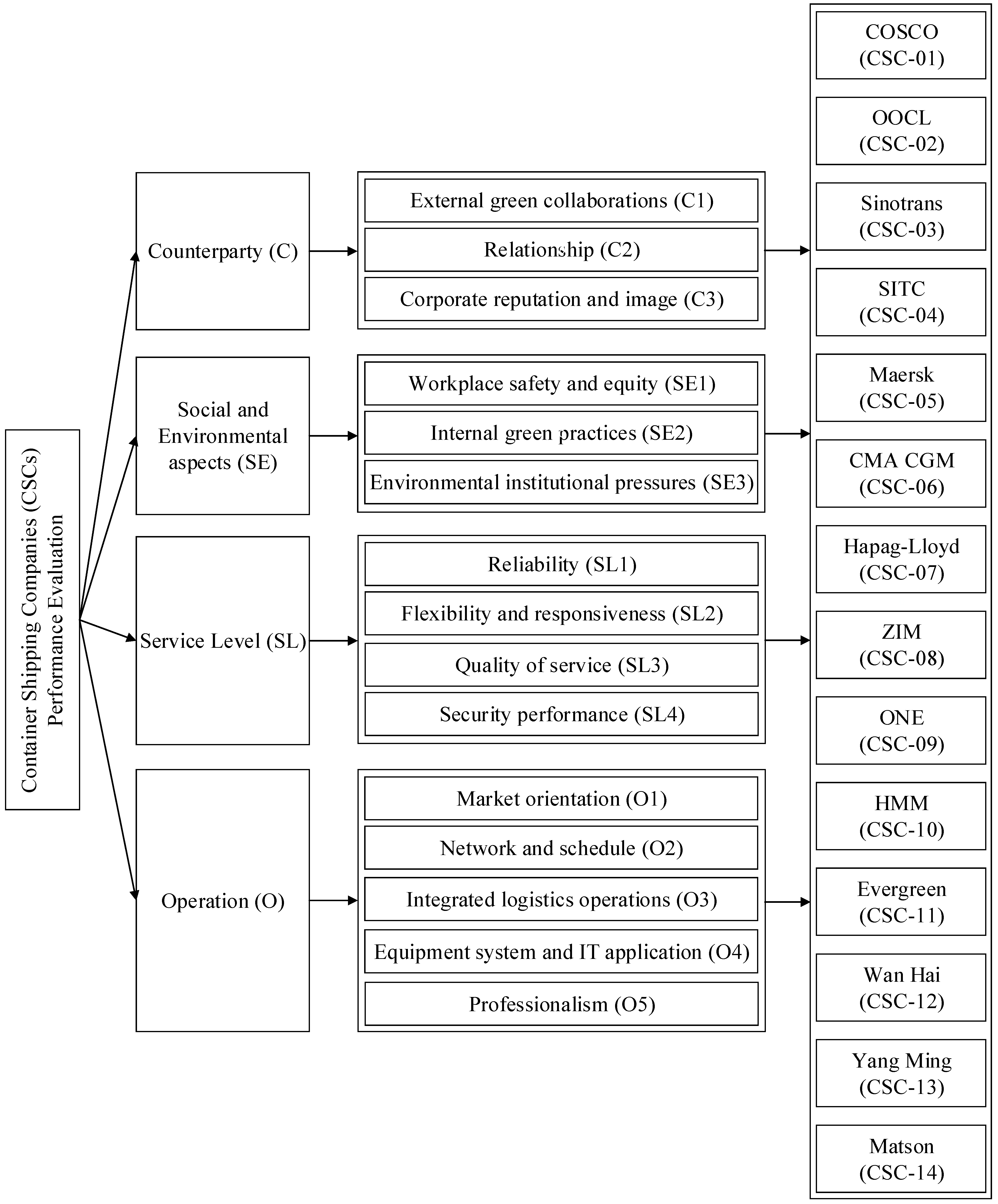
| DMUs | Container Shipping Companies | Symbol | Headquarters | Total TEU | Total Ships | Market Share (%) |
|---|---|---|---|---|---|---|
| CSC-01 | COSCO Shipping Lines | COSCO | China | 2,934,447 | 480 | 11.6 |
| CSC-02 | Orient Overseas Container Line | OOCL | China | 781,779 | 113 | 3.1 |
| CSC-03 | Sinotrans | Sinotrans | China | 45,006 | 31 | 0.2 |
| CSC-04 | SITC Container Lines | SITC | China | 142,602 | 95 | 0.6 |
| CSC-05 | A.P. Moller-Maersk | Maersk | Denmark | 4,279,305 | 736 | 17.0 |
| CSC-06 | CMA-CGM Group | CMA-CGM | France | 3,171,456 | 568 | 12.6 |
| CSC-07 | Hapag-Lloyd | Hapag-Lloyd | Germany | 1,746,772 | 252 | 6.9 |
| CSC-08 | ZIM Integrated Shipping Services | ZIM | Israel | 413,862 | 109 | 1.6 |
| CSC-09 | Ocean Network Express | ONE | Japan | 1,542,261 | 210 | 6.1 |
| CSC-10 | Hyundai Merchant Marine | HMM | South Korea | 819,790 | 75 | 3.3 |
| CSC-11 | Evergreen Marine | Evergreen | Taiwan | 1,477,644 | 204 | 5.9 |
| CSC-12 | Wan Hai Lines | Wan Hai | Taiwan | 422,910 | 149 | 1.7 |
| CSC-13 | Yang Ming Marine Transport | Yang Ming | Taiwan | 662,047 | 90 | 2.6 |
| CSC-14 | Matson | Matson | United States | 68,670 | 29 | 0.3 |
| Dimension | Criteria | Explanation | References |
|---|---|---|---|
| Counterparty (C) | External green collaborations (C1) | Relates to green partnerships and collaborations with suppliers, partners, and clients to jointly decrease environmental impact, reach shared environmental goals, and make collaborative actions. | Yang [25], Di Vaio et al. [26], Lirn et al. [74] |
| Relationship (C2) | Refers to stable cooperation between CSC and their partners, suppliers, and customers to share risks and rewards, regarding reliability, truth, dependence, alliance, compatibility, reciprocity. | Hsu and Ho [27], Yang et al. [75], Tiwari et al. [76] | |
| Corporate reputation and image (C3) | CSC creates a better reputation and brand equity can increase the differentiation advantages of the firm. | Yoon et al. [24], Hsu and Ho [27], Fanam and Ackerly [77] | |
| Social and Environmental aspects (SE) | Workplace safety and equity (SE1) | Refers to the assurance of a safe and equitable workplace for all employees. | Bao et al. [28] |
| Internal green practices (SE2) | Defined as many internal green shipping practices and operations that a CSC can implement and manage independently to reduce the environmental impacts of daily activities. | Yang [25], Di Vaio et al. [26], Lirn et al. [74] | |
| Environmental institutional pressures (SE3) | The adoption and implementation of conventions, directives, regulations, and strategies on container transport to protect the environment. | Yang [25], Di Vaio et al. [26], Lirn et al. [74] | |
| Service Level (SL) | Reliability (SL1) | Refers to on-time performance, responsibility display to customers, accuracy of transshipment, ability to handle cargo at the destination in safe and sound condition, and lower probability of shutting out or roll-over of containers at transshipment port. | Iqbal and Siddiqui [23], Hsu and Ho [27] |
| Flexibility and responsiveness (SL2) | Defined as how fast a shipping line is to cater and adapt to the changing needs and requirements. | Iqbal and Siddiqui [23], Čirjevskis [78] | |
| Quality of service (SL3) | Refers to quality control and inspection for a variety of available and value-added services of a CSC can provide, commitment to continuous improvement. | Yoon et al. [24], Hsu and Ho [27], Yuen and Thai [79] | |
| Security performance (SL4) | Refers to security and safety performance regarding information and cargo during transport. | Hsu and Ho [27], Fanam and Ackerly [77] | |
| Operation (O) | Market orientation (O1) | The ability to gather, share, and respond to market insights with cross-functional coordination to access consumer demands and competitive information. | Tseng and Liao [22] |
| Network and schedule (O2) | This criterion refers to domestic and international service networks, schedule reliability, sufficient sailings, transit timeframe, etc. | Yoon et al. [24], Hsu and Ho [27], Fanam and Ackerly [77], Vernimmen et al. [80] | |
| Integrated logistics operations (O3) | If a CSC effectively integrates logistics operations it means it can reduce transit time and enhance timely delivery, cargo transport security, and flexible tariffs, integrate freight forwarding, logistics operations, customs brokerage, warehousing, and distribution. | Tseng and Liao [22], Hsu and Ho [27], Fanam and Ackerly [77], Vernimmen et al. [80] | |
| Equipment system and IT application (O4) | Capabilities of regular and continuous upgrading the equipment systems, services, and IT applications. | Iqbal and Siddiqui [23], Tseng and Liao [22] | |
| Professionalism (O5) | This dimension is characterized by attributes such as maritime expertise, competence, and experience of an organization. | Hsu and Ho [27] |
| Category | Profile | No. of Respondents |
|---|---|---|
| Education level | Undergraduate | 8 |
| Graduate | 4 | |
| Ph.D. | 3 | |
| Work experience | Between five to ten years | 10 |
| More than ten years | 5 | |
| Work field | Shipping and logistics companies | 6 |
| Port services companies | 2 | |
| Research | 7 |
| Dimension | Left Criteria Is Greater | Right Criteria Is Greater | Dimension | |||||||
|---|---|---|---|---|---|---|---|---|---|---|
| AMI | VHI | HI | SMI | EI | SLI | LI | VLI | ALI | ||
| C | 4 | 3 | 3 | 2 | 2 | 1 | SE | |||
| C | 3 | 2 | 2 | 4 | 4 | SL | ||||
| C | 1 | 2 | 3 | 2 | 4 | 3 | O | |||
| SE | 3 | 3 | 3 | 2 | 1 | 3 | SL | |||
| SE | 2 | 4 | 3 | 2 | 1 | 3 | O | |||
| SL | 1 | 4 | 3 | 3 | 1 | 3 | O | |||
| Dimension | C | SE | SL | O |
|---|---|---|---|---|
| C | 1.000 | 1.171 | 0.417 | 0.491 |
| SE | 0.854 | 1.000 | 0.904 | 0.873 |
| SL | 2.399 | 1.107 | 1.000 | 1.467 |
| O | 2.036 | 1.145 | 0.681 | 1.000 |
| SUM | 6.288 | 4.423 | 3.002 | 3.832 |
| Dimension | C | SE | SL | O | MEAN | WSV | CV |
|---|---|---|---|---|---|---|---|
| C | 0.159 | 0.265 | 0.139 | 0.128 | 0.173 | 0.705 | 4.085 |
| SE | 0.136 | 0.226 | 0.301 | 0.228 | 0.223 | 0.908 | 4.079 |
| SL | 0.381 | 0.250 | 0.333 | 0.383 | 0.337 | 1.390 | 4.127 |
| O | 0.324 | 0.259 | 0.227 | 0.261 | 0.268 | 1.104 | 4.124 |
| Dimension | C | SE | SL | O | ||||||||
|---|---|---|---|---|---|---|---|---|---|---|---|---|
| C | 0.500 | 0.400 | 0.400 | 0.484 | 0.518 | 0.276 | 0.344 | 0.659 | 0.232 | 0.369 | 0.631 | 0.248 |
| SE | 0.441 | 0.553 | 0.282 | 0.500 | 0.400 | 0.400 | 0.433 | 0.573 | 0.259 | 0.429 | 0.576 | 0.264 |
| SL | 0.590 | 0.413 | 0.270 | 0.475 | 0.523 | 0.281 | 0.500 | 0.400 | 0.400 | 0.521 | 0.480 | 0.276 |
| O | 0.552 | 0.443 | 0.280 | 0.484 | 0.512 | 0.288 | 0.406 | 0.588 | 0.270 | 0.500 | 0.400 | 0.400 |
| Dimension | AHP-SF Weight | Calculations to Obtain Crisp Weights | Crisp Weights | ||
|---|---|---|---|---|---|
| C | 0.432 | 0.542 | 0.304 | 11.443 | 0.226 |
| SE | 0.452 | 0.520 | 0.311 | 12.001 | 0.237 |
| SL | 0.525 | 0.451 | 0.312 | 14.151 | 0.279 |
| O | 0.490 | 0.481 | 0.317 | 13.103 | 0.258 |
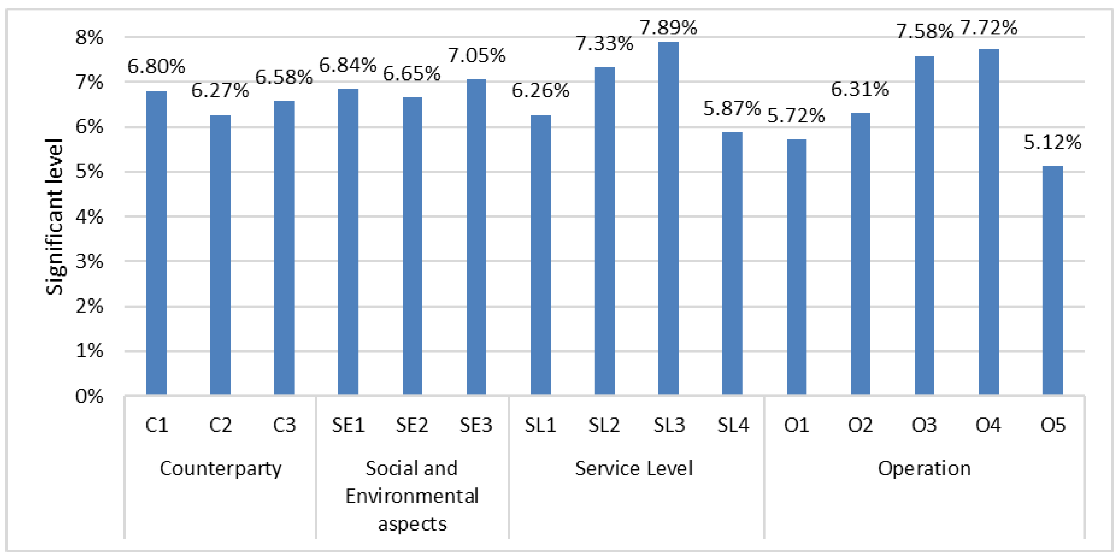
| Criteria | Geometric Mean | Spherical Fuzzy Weights | Crisp Weights | ||||
|---|---|---|---|---|---|---|---|
| External green collaborations (C1) | 0.754 | 0.478 | 0.117 | 0.496 | 0.478 | 0.342 | 0.068 |
| Relationship (C2) | 0.790 | 0.529 | 0.106 | 0.458 | 0.529 | 0.325 | 0.063 |
| Corporate reputation and image (C3) | 0.772 | 0.515 | 0.101 | 0.477 | 0.515 | 0.318 | 0.066 |
| Workplace safety and equity (SE1) | 0.758 | 0.502 | 0.094 | 0.492 | 0.502 | 0.307 | 0.068 |
| Internal green practices (SE2) | 0.769 | 0.506 | 0.096 | 0.480 | 0.506 | 0.310 | 0.066 |
| Environmental institutional pressures (SE3) | 0.740 | 0.482 | 0.107 | 0.510 | 0.482 | 0.327 | 0.071 |
| Reliability (SL1) | 0.794 | 0.544 | 0.091 | 0.454 | 0.544 | 0.301 | 0.063 |
| Flexibility and responsiveness (SL2) | 0.719 | 0.458 | 0.113 | 0.530 | 0.458 | 0.336 | 0.073 |
| Quality of service (SL3) | 0.678 | 0.415 | 0.120 | 0.568 | 0.415 | 0.346 | 0.079 |
| Security performance (SL4) | 0.817 | 0.568 | 0.090 | 0.428 | 0.568 | 0.300 | 0.059 |
| Market orientation (O1) | 0.826 | 0.579 | 0.084 | 0.417 | 0.579 | 0.290 | 0.057 |
| Network and schedule (O2) | 0.789 | 0.524 | 0.099 | 0.459 | 0.524 | 0.314 | 0.063 |
| Integrated logistics operations (O3) | 0.705 | 0.444 | 0.104 | 0.543 | 0.444 | 0.323 | 0.076 |
| Equipment system and IT application (O4) | 0.690 | 0.434 | 0.121 | 0.557 | 0.434 | 0.348 | 0.077 |
| Professionalism (O5) | 0.859 | 0.624 | 0.075 | 0.376 | 0.624 | 0.274 | 0.051 |
| DMUs | Companies | (%) | |||
|---|---|---|---|---|---|
| CSC-01 | COSCO | 0.0773 | 0.0042 | 0.0819 | 96.97 |
| CSC-02 | OOCL | 0.0512 | 0.0025 | 0.0590 | 69.83 |
| CSC-03 | Sinotrans | 0.0377 | 0.0026 | 0.0454 | 53.75 |
| CSC-04 | SITC | 0.0723 | 0.0054 | 0.0760 | 89.97 |
| CSC-05 | Maersk | 0.0807 | 0.0052 | 0.0845 | 100 |
| CSC-06 | CMA-CGM | 0.0711 | 0.0061 | 0.0743 | 87.96 |
| CSC-07 | Hapag-Lloyd | 0.0732 | 0.0059 | 0.0765 | 90.57 |
| CSC-08 | ZIM | 0.0570 | 0.0061 | 0.0603 | 71.32 |
| CSC-09 | ONE | 0.0733 | 0.0054 | 0.0769 | 91 |
| CSC-10 | HMM | 0.0725 | 0.0050 | 0.0765 | 90.50 |
| CSC-11 | Evergreen | 0.0771 | 0.0074 | 0.0798 | 94.41 |
| CSC-12 | Wan Hai | 0.0677 | 0.0053 | 0.0714 | 84.46 |
| CSC-13 | Yang Ming | 0.0663 | 0.0024 | 0.0746 | 88.35 |
| CSC-14 | Matson | 0.0562 | 0.0029 | 0.0630 | 74.59 |
| Variables | Type | Abbreviation | Description | Data Sources |
|---|---|---|---|---|
| Owned-in fleet capacity | Input to cargo model | I1 | Fleet capacity owned by the container carriers (TEU) | Alphaliner website |
| Chartered-in fleet capacity | Input to cargo model | I2 | Fleet capacity of the container carriers chartered from other ship owners (TEU) | Alphaliner website |
| Employee | Input to cargo/eco model | I3 | Number of full-time employees (person) | Annual reports, website, and related reports of each company |
| Operating costs | Input to cargo model | I4 | Cost of goods (services) sold, operating expenses, and overhead expenses (USDm) | Annual reports, website, and related reports of each company |
| Lifting | Output from cargo model/input to eco model | O1/I5 | Measured in terms of volume, through the number of TEUs carried annually (TEU) | Annual reports, website, and related reports of each company |
| EQP | Desirable output from eco model | O2 | Qualitative performance values | COPRAS-G results |
| Revenue | Desirable output from eco model | O3 | Total operating revenue of the companies (USDm) | Annual reports, website, and related reports of each company |
| CO2 emissions | Undesirable output from eco model | O-Bad | Total carbon dioxide emissions released from the companies (thousand tons) | Corporate social responsibility, sustainability reports, website and related reports of each company |
| Variables | Unit | Max | Min | Avg | SD |
|---|---|---|---|---|---|
| Owned-in fleet capacity (I1) | TEU | 2,480,020 | 9247 | 691,761 | 686,332 |
| Chartered-in fleet capacity (I2) | TEU | 1,843,166 | 22,982 | 630,278 | 608,074 |
| Employee (I3) | Person | 83,624 | 1652 | 19,180 | 27,016 |
| Operating costs (I4) | Million USD | 31,804 | 1240 | 10,351 | 9366 |
| Lifting (O1/I5) | TEU | 25,268,000 | 747,200 | 9,056,751 | 7,398,825 |
| Qualitative performance (O2) | % | 100 | 53.75 | 84.55 | 12.24 |
| Revenue (O3) | Million USD | 39,740 | 1685 | 12,657 | 11,514 |
| CO2 emissions (O-Bad) | Thousand tons | 34,207 | 134 | 9701 | 10,334 |
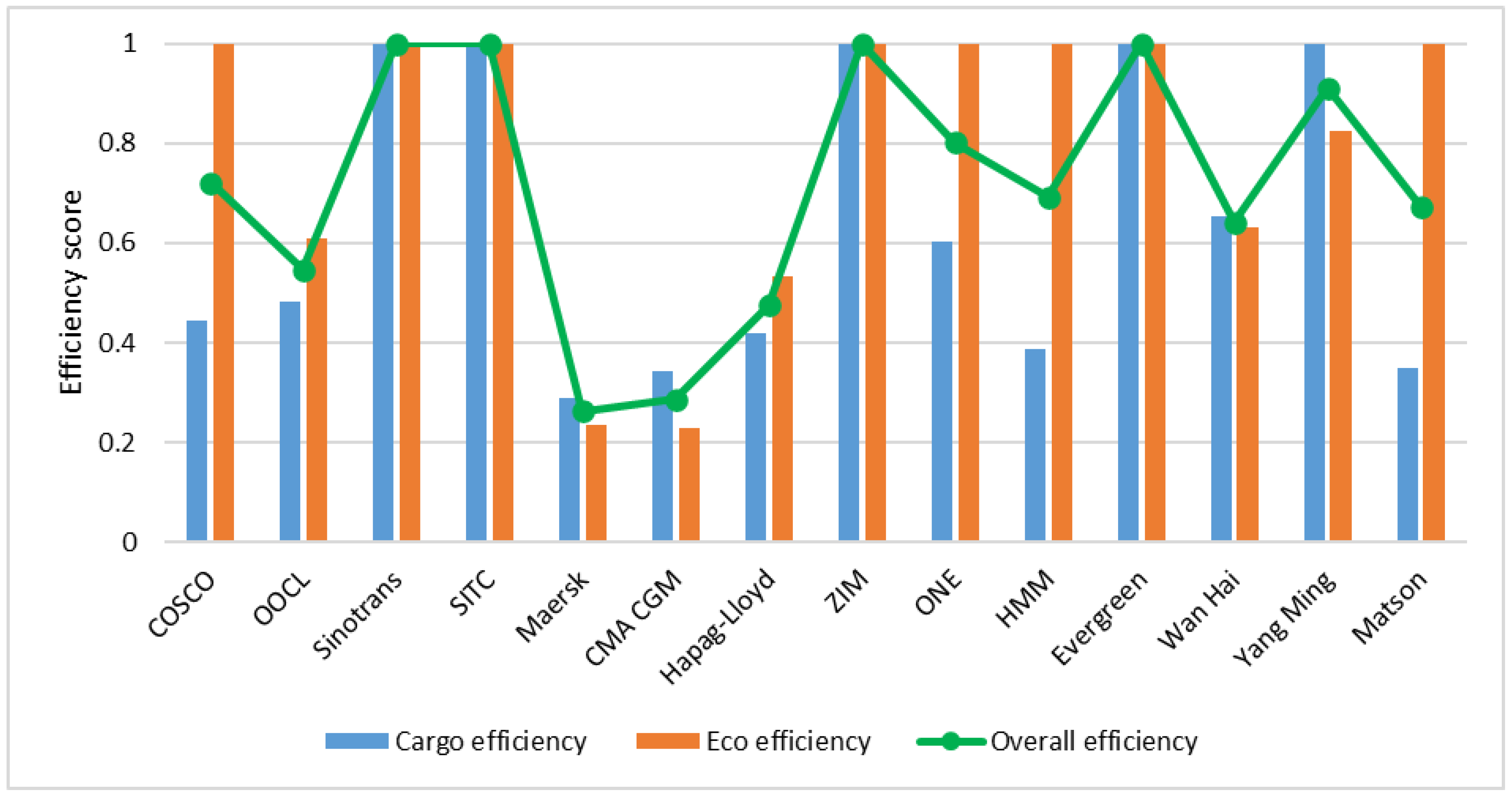
| DMUs | Companies | Cargo Efficiency | Ranking | Eco-Efficiency with EQP | Ranking | Overall Efficiency | Ranking |
|---|---|---|---|---|---|---|---|
| CSC-01 | COSCO | 0.4434 | 9 | 1.0000 | 1 | 0.7217 | 7 |
| CSC-02 | OOCL | 0.4832 | 8 | 0.6098 | 11 | 0.5465 | 11 |
| CSC-03 | Sinotrans | 1.0000 | 1 | 1.0000 | 1 | 1.0000 | 1 |
| CSC-04 | SITC | 1.0000 | 1 | 1.0000 | 1 | 1.0000 | 1 |
| CSC-05 | Maersk | 0.2902 | 14 | 0.2341 | 13 | 0.2622 | 14 |
| CSC-06 | CMA-CGM | 0.3443 | 13 | 0.2281 | 14 | 0.2862 | 13 |
| CSC-07 | Hapag-Lloyd | 0.4185 | 10 | 0.5331 | 12 | 0.4758 | 12 |
| CSC-08 | ZIM | 1.0000 | 1 | 1.0000 | 1 | 1.0000 | 1 |
| CSC-09 | ONE | 0.6036 | 7 | 1.0000 | 1 | 0.8018 | 6 |
| CSC-10 | HMM | 0.3863 | 11 | 1.0000 | 1 | 0.6931 | 8 |
| CSC-11 | Evergreen | 1.0000 | 1 | 1.0000 | 1 | 1.0000 | 1 |
| CSC-12 | Wan Hai | 0.6530 | 6 | 0.6304 | 10 | 0.6417 | 10 |
| CSC-13 | Yang Ming | 1.0000 | 1 | 0.8233 | 9 | 0.9116 | 5 |
| CSC-14 | Matson | 0.3480 | 12 | 1.0000 | 1 | 0.6740 | 9 |
| Average | 0.6407 | 0.7899 | 0.7153 |
Publisher’s Note: MDPI stays neutral with regard to jurisdictional claims in published maps and institutional affiliations. |
© 2022 by the authors. Licensee MDPI, Basel, Switzerland. This article is an open access article distributed under the terms and conditions of the Creative Commons Attribution (CC BY) license (https://creativecommons.org/licenses/by/4.0/).
Share and Cite
Wang, C.-N.; Dang, T.-T.; Nguyen, N.-A.-T.; Chou, C.-C.; Hsu, H.-P.; Dang, L.-T.-H. Evaluating Global Container Shipping Companies: A Novel Approach to Investigating Both Qualitative and Quantitative Criteria for Sustainable Development. Axioms 2022, 11, 610. https://doi.org/10.3390/axioms11110610
Wang C-N, Dang T-T, Nguyen N-A-T, Chou C-C, Hsu H-P, Dang L-T-H. Evaluating Global Container Shipping Companies: A Novel Approach to Investigating Both Qualitative and Quantitative Criteria for Sustainable Development. Axioms. 2022; 11(11):610. https://doi.org/10.3390/axioms11110610
Chicago/Turabian StyleWang, Chia-Nan, Thanh-Tuan Dang, Ngoc-Ai-Thy Nguyen, Chien-Chang Chou, Hsien-Pin Hsu, and Le-Thanh-Hieu Dang. 2022. "Evaluating Global Container Shipping Companies: A Novel Approach to Investigating Both Qualitative and Quantitative Criteria for Sustainable Development" Axioms 11, no. 11: 610. https://doi.org/10.3390/axioms11110610