A Method for Analyzing the Performance Impact of Imbalanced Binary Data on Machine Learning Models

Abstract

Machine learning models may not be able to effectively learn and predict from imbalanced data in the fields of machine learning and data mining. This study proposed a method for analyzing the performance impact of imbalanced binary data on machine learning models. It systematically analyzes 1. the relationship between varying performance in machine learning models and imbalance rate (IR); 2. the performance stability of machine learning models on imbalanced binary data. In the proposed method, the imbalanced data augmentation algorithms are first designed to obtain the imbalanced dataset with gradually varying IR. Then, in order to obtain more objective classification results, the evaluation metric AFG, arithmetic mean of area under the receiver operating characteristic curve (AUC), F-measure and G-mean are used to evaluate the classification performance of machine learning models. Finally, based on AFG and coefficient of variation (CV), the performance stability evaluation method of machine learning models is proposed. Experiments of eight widely used machine learning models on 48 different imbalanced datasets demonstrate that the classification performance of machine learning models decreases with the increase of IR on the same imbalanced data. Meanwhile, the classification performances of LR, DT and SVC are unstable, while GNB, BNB, KNN, RF and GBDT are relatively stable and not susceptible to imbalanced data. In particular, the BNB has the most stable classification performance. The Friedman and Nemenyi post hoc statistical tests also confirmed this result. The SMOTE method is used in oversampling-based imbalanced data augmentation, and determining whether other oversampling methods can obtain consistent results needs further research. In the future, an imbalanced data augmentation algorithm based on undersampling and hybrid sampling should be used to analyze the performance impact of imbalanced binary data on machine learning models.

1. Introduction

In the fields of data mining and machine learning, imbalanced data classification is a ubiquitous natural phenomenon. Imbalanced data classification is a kind of supervised learning, which means that the distribution of response variables in the dataset varies greatly in different classes. In binary or multiclass datasets affected by imbalanced data classification, a response variable with fewer samples is referred to as a positive class or a minority class, whereas a response variable with more samples is known as a negative class or a majority class. Due to the machine learning models being based on situations in which the data distribution is relatively balanced, these machine learning models may experience different degrees of defects when faced with imbalanced data classification and may thus become inefficient [1]. For example, suppose there is a patient dataset containing 990 normal patients and 10 cancer patients. If we do not modify the machine learning model or improve the distribution of data and use the machine learning model directly, it will tend to think that all patients in the dataset are normal patients. This can lead to a terrible situation in which cancer patients missed the optimal treatment time because they cannot be accurately predicted, thus endangering their lives or even death. Therefore, enhancing the analysis and understanding of machine learning models for imbalanced data classification has important theoretical significance and application value [2].

Current studies on the imbalanced data classification issues are mainly concerned with two methods [3]. The first involves newly designing or improving the machine learning models, which generally entails reducing the sensitivity of the classification algorithm to the imbalanced data. Typically, either ensemble learning is used to increase the robustness of the machine learning models [4] or a cost-sensitive learning method [5] is used to make the cost of misclassifying the minority class higher than that of misclassifying the majority class. The second approach is to use a sampling method to balance the dataset on the data level, mainly via oversampling [6,7], undersampling [3] or hybrid sampling [8]. The purpose of oversampling is to increase the number of samples in the minority class, thus improving the distribution of data among classes. Undersampling has the same purpose as oversampling, but instead removes samples from the majority class. Finally, hybrid sampling is intended to balance the dataset by combining the two aforementioned sampling methods.

This study aims to provide a method to analyze the performance impact of imbalanced binary data on machine learning models. Hence, proposing new techniques addressing imbalanced data classification is not the focus. The method proposed in this study not only analyzes the relationship between varying performance in machine learning models and IR, but also analyzes the performance stability of the machine learning models on the imbalanced datasets. The main contributions of this study can be summarized as follows.

(1) To obtain the imbalanced dataset with gradually varying IR and belonging to the same distribution, this study proposes three different augmentation algorithms of imbalanced data by combining the oversampling method, the undersampling method and the hybrid sampling method, respectively.

(2) This study proposes a performance evaluation metric AFG by analyzing and combining evaluation metrics AUC, F-measure and G-mean.

(3) Our comparative study systematically analyzes the relationship between varying performance in machine learning models and IR, as well as the performance stability of eight machine learning models on 48 benchmark imbalanced datasets, which can provide an important reference value for imbalanced data classification application developers and researchers.

The remainder of this study is organized as follows. Section 2 describes the proposed approach in detail. Experiment settings are given in Section 3, and the experimental results are discussed in Section 4. The related works are discussed in Section 5. Finally, Section 6 briefly summarizes our study and presents the conclusions.

2. Proposed Method

The overall framework of the method for analyzing the performance impact of imbalanced binary data on machine learning models is shown in Figure 1.

Specifically, in the framework, a new set of imbalanced data with decreasing IR is augmented based on the augmentation algorithms in the first. How to augment an imbalanced dataset with decreasing IR will be described in detail in Section 2.1. Then, in Section 2.2, in order to obtain the relationship between varying performance in machine learning models and IR, we use AFG, the arithmetic mean of AUC, F-measure and G-mean, to evaluate the classification performance of machine learning models. Finally, in Section 2.3, the performance stability of machine learning models on imbalanced datasets is evaluated by combining AFG and CV. Meanwhile, statistical tests are applied to further verify whether the performance stability of these machine learning models is significantly different.

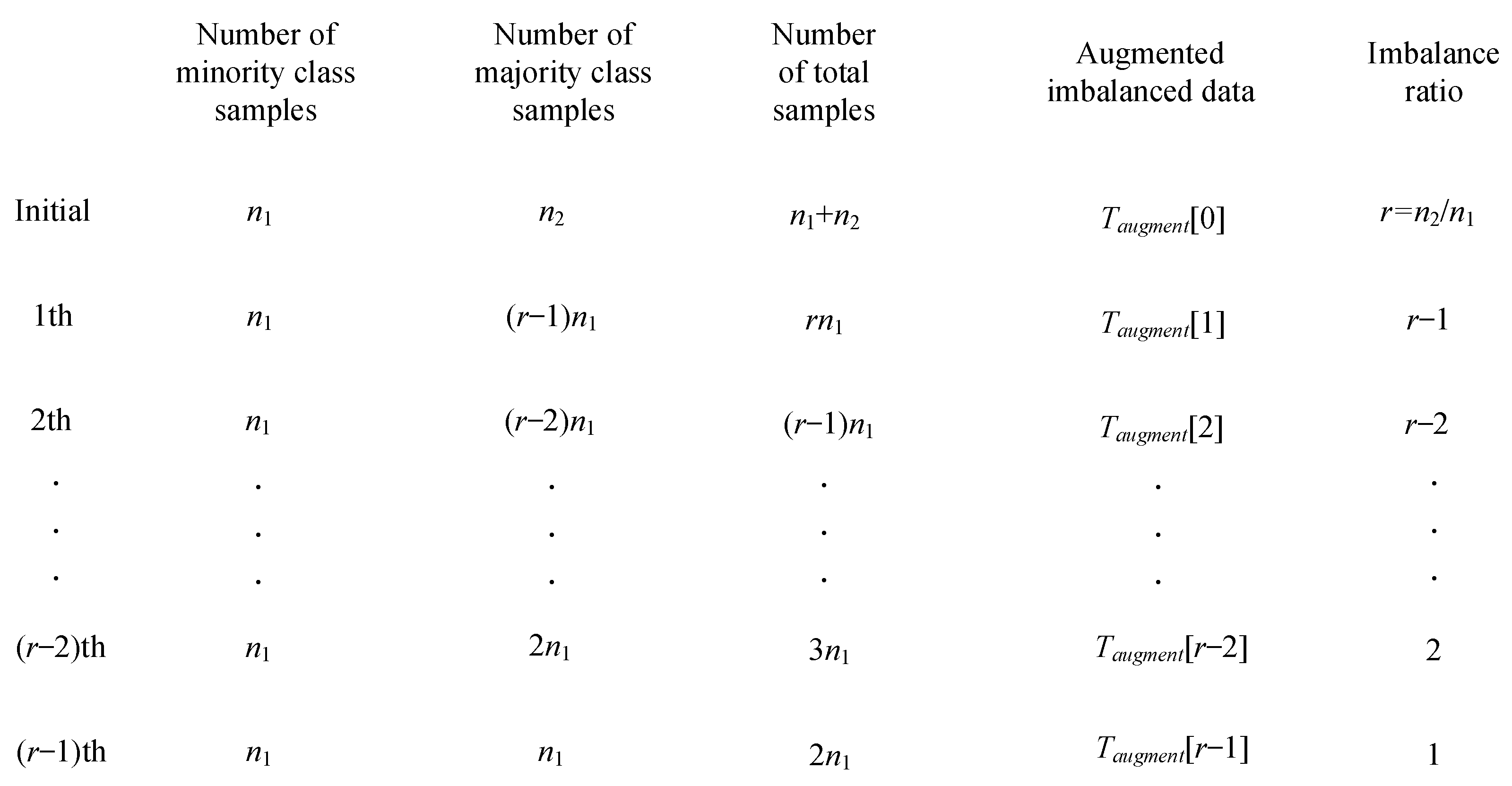
2.1. Imbalanced Data Augmentation Algorithms

Only when an imbalanced dataset with gradually varying IR is obtained can the relationship between varying performance in machine learning models and IR be analyzed. Although it can be simply achieved by collecting imbalanced data with different IRs, because different imbalanced data have different distributions, it is impossible to effectively analyze the relationship between varying performance in machine learning models and IR. Therefore, this study proposes three different augmentation algorithms for imbalanced data based on the oversampling method, the undersampling method and the hybrid sampling method, respectively, so as to obtain a set of imbalanced data from the same distribution, with decreasing IR.

First, the imbalanced data augmentation algorithm based on the oversampling method is introduced. After applying Algorithm 1, the augmented imbalanced dataset with decreasing IR can be obtained.

Algorithm 1 Oversampling-based imbalanced data augmentation

Input:T: Original imbalanced data.

Output: Taugment: Augmented imbalanced dataset.

Procedure Begin

T ← Tmajority ∪ Tminority n1 ← size of Tminority n2 ← size of Tmajority r ← int (n2/n1) fori = 0 to r − 1 do  oversampling ratio ← 1/(r − i)  generated minority class samples ← oversampling approach (T, oversampling ratio)  Taugment[i] ← T ∪ generated minority class samples  return Taugment[i] end for returnTaugment End

Algorithm 1 first divides the original imbalanced data into majority class samples T_majority and minority class samples T_minority according to the class label of samples. Among them, the number of minority class samples is n₁, and the number of majority class samples is n₂. Then, the IR of the original imbalanced data T is calculated and denoted with r; note that r is the value rounded down. Traversing r, each traversal will calculate the oversampling ratio. According to the oversampling ratio and original imbalanced data T, the oversampling approach is used to generate minority class samples, merge the generated minority class samples with the original imbalanced data T to get new imbalanced data and the above steps are repeated until the end of the loop to finally obtain the augmented imbalanced dataset T_augment (a group of imbalanced datasets with decreasing IR). The relationship between the augmentation process of imbalanced data and IR change in Algorithm 1 is shown in Figure 2.

Then, the imbalanced data augmentation algorithm based on the undersampling method is introduced. After applying Algorithm 2, the augmented imbalanced dataset with decreasing IR can be obtained.

Algorithm 2 Undersampling based imbalanced data augmentation

Input:T: Original imbalanced data.

Output: Taugment: Augmented imbalanced dataset.

Procedure Begin

T ← Tmajority ∪ Tminority n1 ← size of Tminority n2 ← size of Tmajority r ← int (n2/n1) fori = 0 to r − 1 do  undersampling ratio ← 1/(r − i)  deleted majority class samples ← undersampling approach (T, undersampling ratio)  Taugment[i] ← T—deleted majority class samples  return Taugment[i] end for returnTaugment End

Similarly, Algorithm 2 first divides the original imbalanced data into majority class samples T_majority and minority class samples T_minority according to the class of samples. Among them, the number of minority class samples is n₁, and the number of majority class samples is n₂. Then, the IR of the original imbalanced data T is calculated and denoted with r; note that r is the value rounded down again. Traversing r, each traversal will calculate the undersampling ratio. According to the undersampling ratio and original imbalanced data T, the undersampling approach is used to delete majority class samples, remove deleted majority class samples from the original imbalanced data T to get new imbalanced data and the above steps are repeated until the end of the loop to finally obtain the augmented imbalanced dataset T_augment (a group of imbalanced datasets with decreasing IR). The relationship between the augmentation process of imbalanced data and IR change in Algorithm 2 is shown in Figure 3.

Last, the imbalanced data augmentation algorithm based on the hybrid sampling method is introduced. After applying Algorithm 3, the augmented imbalanced dataset with decreasing IR can be obtained.

Algorithm 3 Hybrid sampling based imbalanced data augmentation

Input:T: Original imbalanced data.

Output: Taugment: Augmented imbalanced dataset.

Procedure Begin

T ← Tmajority ∪ Tminority n1 ← size of Tminority n2 ← size of Tmajority r ← int (n2/n1) fori = 0 to r − 1 do  oversampling ratio ← (n1 + n2)/rn2  undersampling ratio ← rn1/[(n1 + n2)(r − 1)]  generated minority class samples ← oversampling approach (T, oversampling ratio)  deleted majority class samples ← undersampling approach (T, undersampling ratio)  Taugment[i] ← generated minority class samples ∪ T—deleted majority class samples  return Taugment[i] end for returnTaugment End

Algorithm 3 first divides the original imbalanced data into majority class samples T_majority and minority class samples T_minority according to the class of samples. Among them, the number of minority class samples is n₁, and the number of majority class samples is n₂. Then, the IR of the original imbalanced data T is calculated and denoted with r; note that r is the value rounded down. Traversing r, each traversal will calculate the oversampling ratio and the undersampling ratio. According to the oversampling ratio, undersampling ratio and original imbalanced data T, the oversampling approach and undersampling approach are used to generate the minority class samples and delete the majority class samples, respectively. The generated minority class samples are merged and the deleted majority class samples are removed from the original imbalanced data T to obtain new imbalanced data and the above steps are repeated until the end of the loop, to finally obtain the augmented imbalanced dataset with decreasing IR. The relationship between the augmentation process of imbalanced data and IR change in Algorithm 3 is shown in Figure 4.

It should be noted that the three imbalanced data augmentation algorithms have good flexibility. This is because the resampling methods of the three augmentation algorithms are not fixed, and can be arbitrary oversampling, undersampling and hybrid sampling methods, so they are represented in italics. Meanwhile, the above three augmentation algorithms have the same purpose and are all designed to augment imbalanced data into a group of imbalanced datasets with decreasing IR. As long as the resampling methods in the above augmentation algorithms are good enough, the augmented data and the original imbalanced data belong to the same distribution. Because the SMOTE (synthetic minority oversampling technique) [6] is a classical and widely used oversampling method in the studies of imbalanced data classification [9,10,11], this study uses a SMOTE-based augmentation algorithm to augment the imbalanced binary data.

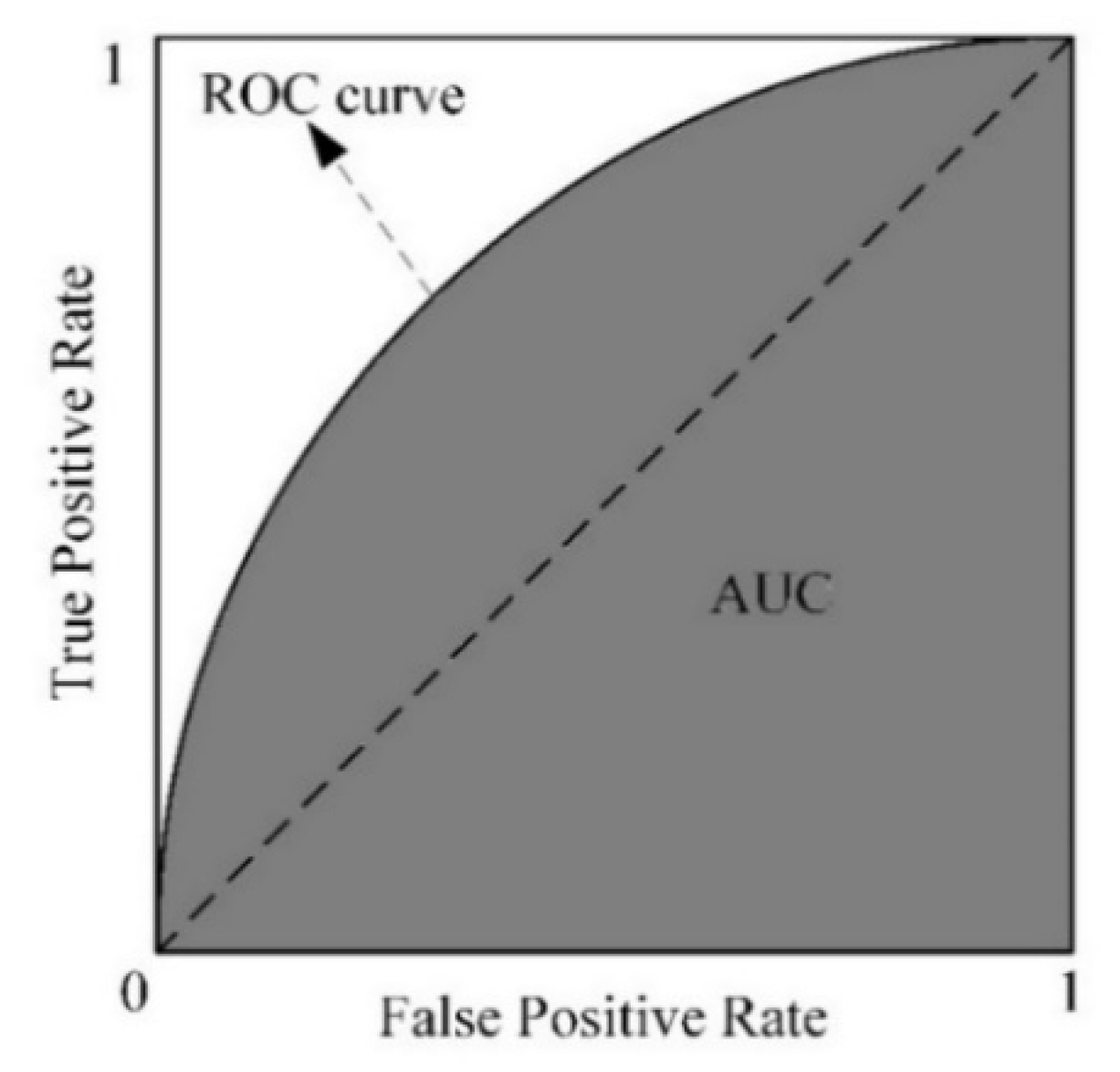
2.2. Performance Evaluation Metric

The evaluation metrics AUC, F-measure and G-mean are widely used to evaluate the classification performance of machine learning models for imbalanced data classification [12,13,14]. To facilitate the introduction of the calculation rules of the evaluation metrics, the confusion matrix was first established, as detailed in

Table 1. Binary classification confusion matrix.

	Predicted Positive	Predicted Negative
Actual positive	True positives (TP)	False negatives (FN)
Actual negative	False positives (FP)	True negatives (TN)

.

The rows and columns in Table 1 represent the real and predicted sample classes, respectively. True positive (TP) indicates a positive sample predicted as a positive class by the model, false negative (FN) represents a positive sample predicted as a negative class by the model, false positive (FP) represents a negative sample predicted as a positive class by the model and true negative (TN) represents a negative sample predicted as a negative class by the model. The above three performance evaluation metrics are defined as follows.

The larger the AUC, the more effective the classifier. Figure 5 illustrates the calculation of the AUC on a two-dimensional chart, where the gray area is the AUC value.

In Figure 5, the x-axis represents the false positive rate (FPR); that is, the proportion of misclassified negative cases relative to the total number of negative cases. The y-axis represents the true positive rate (TPR); that is, the proportion of correctly predicted positive cases relative to the total number of positive cases. As the ROC curve depends on the classification threshold, the AUC is a useful performance evaluation metric of the classifier because it is independent of the decision criterion [15].

$$F\_measure=\frac{\left(1+{\beta }^2\right)\cdot recall\cdot precision}{{\beta }^2\cdot recall+precision},$$

(1)

where recall = $\frac{TP}{TP+FN}$, precision = $\frac{TP}{TP+FP}$, (β = 1 in this study).

$$G\_mean=\sqrt{recall\times specificity},$$

(2)

where specificity = $\frac{TN}{TN+FP}$.

Although the above three evaluation metrics are widely used in the field for imbalanced data classification, their three focuses are different. For example, the AUC evaluation metric focuses on optimizing TPR and 1-FPR at the same time, the F-measure evaluation metric focuses on optimizing recall and precision at the same time, and the G-mean evaluation metric focuses on optimizing the product of recall and specificity. The optimal values of the above three evaluation metrics are all 1. Meanwhile, in order to comprehensively consider the different focuses of the three evaluation metrics to obtain a more objective classification performance result, we use AFG, the arithmetic mean of AUC, F-measure and G-mean as the performance evaluation metric of machine learning models on imbalanced datasets.

$$\begin{gathered} \mathrm{AFG}=\left(w_1·AUC+w_2·F\_measure+w_3·G\_mean\right)/3, \\ (w_1=w_2=w_2=1 \mathrm{in} \mathrm{this} \mathrm{study}) \end{gathered}$$

(3)

2.3. Performance Stability Evaluation Method

Because the average performance of different machine learning models is greatly different on the same imbalanced data, the standard deviation of performance cannot be used to directly measure the discreteness of the performance of each machine learning model. Therefore, in order to avoid affecting the comparison of imbalanced data dispersion, the combination of CV [16,17] and AFG was proposed to evaluate the dispersion of the machine learning models in an imbalanced dataset.

$$P_{\mathrm{AFG}}=\left\{{\mathrm{AFG}}_0,{\mathrm{AFG}}_1,\dots ,{\mathrm{AFG}}_{r-1}\right\},$$

(4)

$${\mu }_{\mathrm{AFG}}={{\displaystyle \sum }}_{i=0}^{r-1}{\mathrm{AFG}}_i/r,$$

(5)

$${\sigma }_{\mathrm{AFG}}=\sqrt{{{\displaystyle \sum }}_{i=0}^{r-1}{({\mathrm{AFG}}_i-{\mu }_{\mathrm{AFG}})}^2/r},$$

(6)

$$C{V}_{\mathrm{AFG}}=\left({\sigma }_{\mathrm{AFG}}/{\mu }_{\mathrm{AFG}}\right)\times 100\%,$$

(7)

where μ_AFG and σ_AFG represent the average value and standard deviation of all AFG in the P_AFG set. CV_AFG represents the CV of P_AFG. The larger the CV_AFG, the greater the degree of dispersion of the performance metric. From Equation (7), it can be seen that the CV_AFG is affected by both the average and the standard deviation at the same time, and the larger CV_AFG, the greater the impact of imbalanced data on machine learning models, and the more unstable the performance of the machine learning model on the imbalanced data. Generally speaking, when CV_AFG is greater than 10%, the performance of the machine learning model on imbalanced data can be considered to be relatively unstable, while when CV_AFG is less than 10%, the performance of the machine learning model on imbalanced data can be considered to be relatively stable.

3. Experiment Settings

The benchmark imbalanced data are described in Section 3.1. We briefly introduce the eight machine learning models for training and classifying imbalanced data in Section 3.2. Section 3.3 explains the experimental flow design. Finally, Section 3.4 introduces statistical test method.

3.1. Benchmark Dataset

This study experimented on 48 different benchmark imbalanced datasets in multiple fields extracted from the UCI Machine Learning Repository, Data Hub and a part of Network Intrusion Data; these imbalanced data are publicly available on the corresponding web pages (https://archive.ics.uci.edu/ml/datasets.php, https://datahub.io/machine-learning, accessed on 1 January 2022).

Table 2. Characteristics of the imbalanced data used in the experiment.

ID	Dataset	Instances	Features	Minority Class	Majority Class	Minority Instances	Majority Instances	IR
1	Zoo	101	17	7	all other	10	91	9.1
2	Balance	625	4	B	all other	49	576	11.755
3	Dermatology	358	34	6	all other	20	338	16.9
4	Wilt	4839	5	w	n	261	4578	17.540
5	Satimage0vs12	6430	36	2	all other	703	5727	8.147
6	Satimage1vs02	6430	36	4	all other	625	5805	9.288
7	Satimage2vs01	6430	36	5	all other	707	5723	8.095
8	Ecoli0vs1	336	7	imU	all other	35	301	8.6
9	Ecoli1vs0	336	7	om	all other	20	316	15.8
10	Glass0vs12	214	9	3	all other	17	197	11.588
11	Glass1vs02	214	9	5	all other	13	201	15.462
12	Glass2vs01	214	9	6	all other	9	205	22.778
13	Pageblocks0vs1	5473	10	2	all other	329	5144	15.635
14	Pageblocks1vs0	5473	10	5	all other	115	5358	46.591
15	Yeast0vs1234	1484	8	VAC	all other	30	1454	48.467
16	Yeast1vs0234	1484	8	EXC	all other	35	1449	41.4
17	Yeast2vs0134	1484	8	ME1	all other	44	1440	32.727
18	Yeast3vs0124	1484	8	ME2	all other	51	1433	28.098
19	Yeast4vs0123	1484	8	ME3	all other	163	1321	8.104
20	Zernike0vs1-9	2000	47	1	all other	200	1800	9
21	Zernike1vs0_2-9	2000	47	2	all other	200	1800	9
22	Zernike2vs01_3-9	2000	47	3	all other	200	1800	9
23	Zernike3vs0-2_4-9	2000	47	4	all other	200	1800	9
24	Zernike4vs0-3_5-9	2000	47	5	all other	200	1800	9
25	Zernike5vs0-4_6-9	2000	47	6	all other	200	1800	9
26	Zernike6vs0-5_7-9	2000	47	7	all other	200	1800	9
27	Zernike7vs0-6_89	2000	47	8	all other	200	1800	9
28	Zernike8vs0-7_9	2000	47	9	all other	200	1800	9
29	Zernike9vs0-8	2000	47	10	all other	200	1800	9
30	Libra0vs1-14	360	90	1	all other	24	336	14
31	Libra1vs0_2-14	360	90	2	all other	24	336	14
32	Libra2vs01_3-14	360	90	3	all other	24	336	14
33	Libra3vs0-2_4-14	360	90	4	all other	24	336	14
34	Libra4vs0-3_5-14	360	90	5	all other	24	336	14
35	Libra5vs0-4_6-14	360	90	6	all other	24	336	14
36	Libra6vs0-5_7-14	360	90	7	all other	24	336	14
37	Libra7vs0-6_8-14	360	90	8	all other	24	336	14
38	Libra8vs0-7_9-14	360	90	9	all other	24	336	14
39	Libra9vs0-8_10-14	360	90	10	all other	24	336	14
40	Libra10vs0-9_11-14	360	90	11	all other	24	336	14
41	Libra11vs0-10_12-14	360	90	12	all other	24	336	14
42	Libra12vs0-11_13-14	360	90	13	all other	24	336	14
43	Libra13vs0-12_14	360	90	14	all other	24	336	14
44	Libra14vs0-13	360	90	15	all other	24	336	14
45	KDDCup1999	13,228	41	all other	normal	3228	10,000	3.098
46	NSL-KDD2009	13,158	41	all other	normal	3158	10,000	3.167
47	CSE-CIC-IDS2018	12,403	78	all other	normal	2403	10,000	4.161
48	CICIDS17	12,180	78	all other	normal	2180	10,000	4.587

summarizes the 48 imbalanced datasets with different IR, including the total number of instances, numbers of features, class names and number of instances belonging to the minority. To obtain multiple binary imbalanced data, we refer to the method in similar imbalanced data classification studies [18,19,20], and transform multiclass imbalanced data in the UCI and Data Hub into binary imbalanced data by combining one or more classes. As shown in Table 2, although some imbalanced datasets are the same imbalanced data, with different versions, they are different. For example, Yeast0vs1234, Yeast1vs0234 and Yeast2vs0134 are three imbalanced data versions of Yeast, which contain different samples and classes. In Yeast0vs1234, the positive class samples (minority class) belong to class 0, and the negative class samples belong to classes 1, 2, 3 and 4 (majority class samples). In Yeast1vs0234, the positive class samples (minority class) belong to class 1 and the negative class samples belong to classes 0, 2, 3 and 4 (majority class samples). In Yeast2vs0134, the positive class samples (minority class) belong to class 2 and the negative class samples belong to classes 0, 1, 3 and 4 (majority class samples).

3.2. Machine Learning Models

In order to compare the performance stability between machine learning models, this study uses eight widely used machine learning models, including Gaussian Naive Bayes (GNB) [21], Bernoulli naive Bayes (BNB) [22], K-nearest neighbor (KNN) [23], logistic regression (LR) [24], random forest (RF) [25], decision tree (DT) [26], gradient boosting decision tree [27] and support vector classifier (SVC) [28], used as classification algorithms to train and predict imbalanced data. These machine learning models were implemented based on the Python library Scikit-Learn [29] with default settings employed.

3.3. Experimental Flow Design

To prevent the testing set from being affected by an imbalanced data augmentation algorithm, it was isolated from the training set during preprocessing. Therefore, we only perform an imbalanced data augmentation algorithm on the training set. We randomly selected 10% of the original imbalanced data as the testing set, and the remaining 90% as the training set. Then, IR is calculated according to the number of majority class and minority class samples. Next, the training set is augmented based on Algorithm 1, IR and SMOTE. Finally, the performance of the machine learning models is evaluated based on AFG and CV_AFG. Figure 6 shows the experimental flowchart for each imbalanced dataset. With each different IR, the experiment was repeated 100 times to reduce the impact of bias caused by the randomness of the experiment.

3.4. Statistical Test Method

This study employed non-parametric testing to analyze and compare whether there are significant differences in the performance stability of machine learning models on imbalanced datasets. These tests have been used in several empirical studies and are highly recommended in the field of machine learning and data mining [20,30] to confirm experimental results. The non-parametric test procedure consists of three steps. First, ranking scores are computed by assigning a rank score to each machine learning model in each imbalanced dataset. Because the smaller the CV_AFG, the more stable the performance of the machine learning model, therefore 8 is assigned to the most unstable machine learning model, 7 to the second unstable machine learning model, and so on. The ranking score of the best stable machine learning model is 1. Then, the mean ranking scores of eight machine learning models on 48 imbalanced datasets are computed. Next, the Friedman test is used to determine whether these machine learning models deliver the same performance stability. If performance stability differs, the hypothesis that all machine learning models have the same performance stability is rejected; if the performance stability of the machine learning model is significantly different, a post hoc test is needed to further distinguish each machine learning model. Finally, when the hypothesis that all machine learning models have the same performance stability is rejected, the Nemenyi post hoc test is applied to check whether the control machine learning model (usually the most stable one) significantly outperforms the remaining machine learning models. The Nemenyi post hoc procedures enable calculating the critical distance of the mean ranking score difference. If the difference between the mean ranking scores of the two machine learning models exceeds the critical distance, the hypothesis that the performance stability of the two machine learning models is the same is rejected at a specified level of significance α (i.e., there exist significant differences); in this study, α = 0.05.

4. Experimental Results and Discussion

This section presents the experimental results of 48 different imbalanced datasets for eight machine learning models. Section 4.1 shows the experimental results of the relationship between varying performance in machine learning models and IR. The performance stability results of eight machine learning models on 48 different imbalanced datasets are presented in Section 4.2, and Section 4.3 presents the statistical test results.

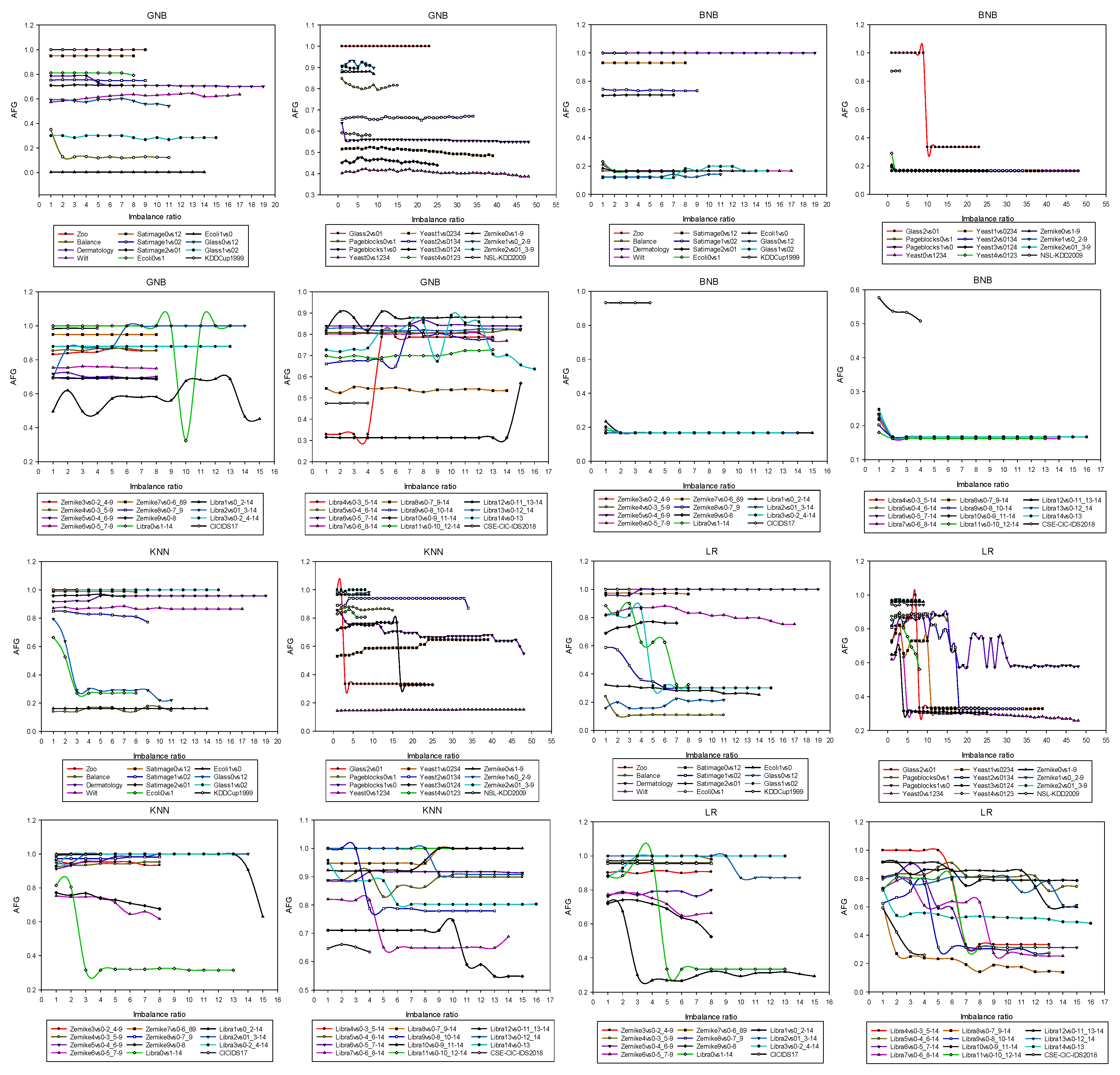
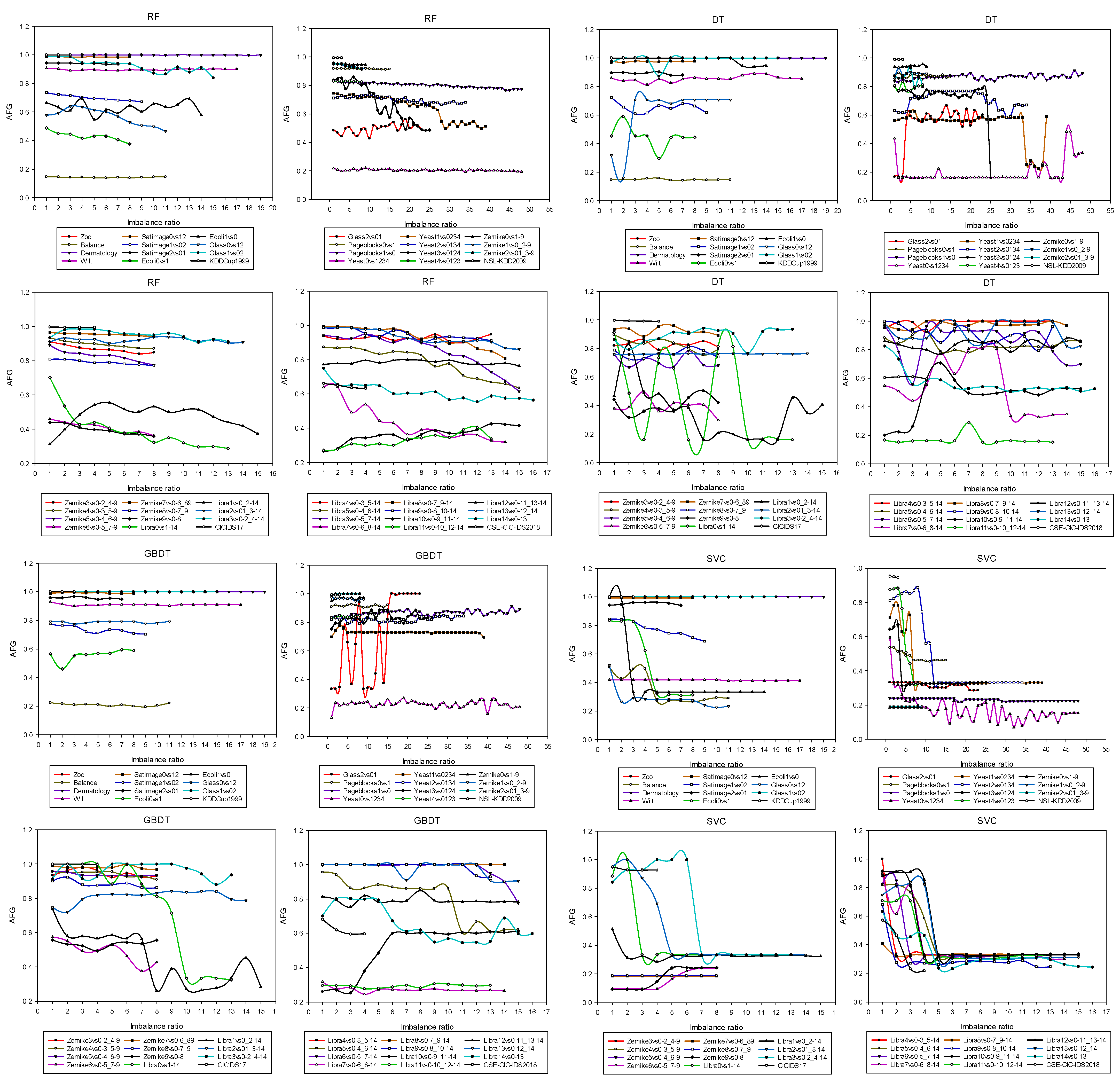
4.1. Relationship between Varying Performance in Machine Learning Models and IR

In order to analyze the relationship between varying performance in machine learning models and IR, a line chart is used to display the experimental data. As shown in Figure 7 and Figure 8, the x-axis and y-axis represent the IR and values of AFG, respectively. Similarly, 48 different imbalanced datasets will be divided into four groups for comparison, each group including 11 different imbalanced datasets. Therefore, each small graph in Figure 7 and Figure 8 represents the relationship between AFG variation and the IR of a machine learning model on 48 imbalanced datasets. At the same time, the IR of different imbalanced data is different, so the lines in the figures have different lengths.

From Figure 7 and Figure 8 we can observe:

(1) With the gradual increase in the IR, the AFG performance of all eight machine learning models on most imbalanced datasets shows a downward trend. In addition, there are two main situations for this downward trend. One is that the AFG performance decreases sharply at first, and then the AFG performance gradually decreases as the IR gradually increases. Another situation is that as the IR gradually increases, the AFG performance always gradually decreases.

(2) On a few imbalanced datasets, with the gradual increase in the IR, the AFG performance of some machine learning models increases without degradation. We speculate that there are two reasons for this. One is that the imbalanced data is too complicated to train, and the other is that we assume that the data generated by the oversampling method belongs to the original imbalanced data distribution. However, the real situation is that the oversampling method may have some limitations, making the quality of minority class samples generated during each imbalanced data augmentation different, which leads to this situation.

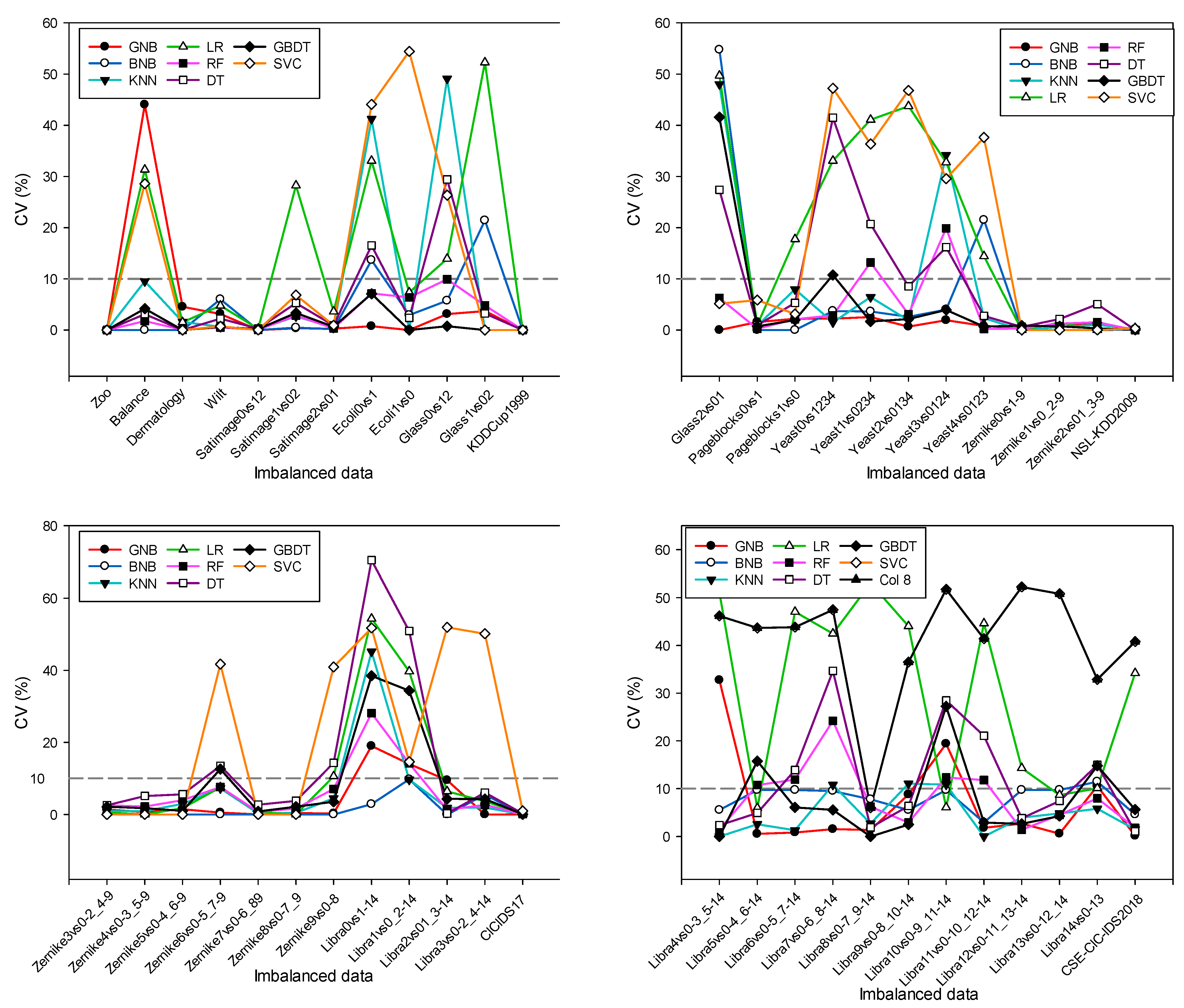
4.2. Performance Stability Results

Figure 8 shows the coefficient of variation CV_AFG (%) of eight machine learning models on 48 imbalanced datasets. The larger the CV_AFG, the greater the influence of imbalanced data on the machine learning model, and the more unstable the performance. In order to compare the performance stability of different machine learning models on different imbalanced data more clearly, 48 different imbalanced datasets will be divided into four groups for comparison, each group including 12 different imbalanced datasets.

As shown in Figure 9, the x and y axes of each plot represent the different imbalanced data with different IRs and CV_AFG scores, respectively. Among them, eight different colors represent eight different machine learning models. It should be noted that since the CV_AFG value of a few machine learning models is 0, this indicates that the performance of the machine learning model on the imbalanced dataset is very stable, for example, the imbalanced dataset Zoo.

Since the larger the CV_AFG, the more unstable the performance, conversely, the smaller the CV_AFG, the more stable the performance. From Figure 9, the following results are obtained:

(1) LR, DT and SVC have relatively more imbalanced data with CV_AFG greater than 10% in 48 different imbalanced datasets, indicating that these three machine learning models are easily affected by the imbalanced data. Among them, the SVC is the most vulnerable to the impact of imbalanced data, because, on the one hand, the imbalanced data with CV_AFG greater than 10% is the highest in SVC, and, on the other hand, the value of CV_AFG in SVC is also relatively the largest, and the larger the CV_AFG, the more unstable the performance.

(2) GNB, BNB, KNN, RF and GBDT have relatively less imbalanced data with CV_AFG greater than 10% in 48 different imbalanced datasets, indicating that these five machine learning models are not susceptible to imbalanced data. Among them, the machine learning model BNB is the most stable because the imbalanced data with CV_AFG greater than 10% is the lowest in BNB.

(3) The distribution of different imbalanced data can also affect the performance of machine learning models. For example, more than half of the machine learning models had a CV_AFG greater than 10% on eight imbalanced data (Ecoli0vs1, Glass2vs01, Yeast3vs0124, Libra0vs1-14, Libra1vs0_2-14, Libra7vs0-6_8-14, Libra10vs0-9_11-14 and Libra14vs0-13), showing unstable performance. In other words, compared with other imbalanced data among the 48 imbalanced datasets, these eight imbalanced data are likely to affect the performance of the machine learning models. Especially for the imbalanced data Libra-0, except for BNB, the CV_AFG of the other seven classification algorithms are all greater than 10%. It can be inferred that these eight imbalanced data are relatively complex and difficult to train. In addition, the results of the performance stability evaluation are statistically confirmed by statistical tests.

4.3. Statistical Test Results

The mean ranking scores of eight machine learning models on 48 imbalanced datasets are listed in

Table 3. Mean ranking scores of eight machine learning models with CV_AFG on 48 imbalanced datasets. Bold values indicate the best machine learning model for each row.

Algorithms	GNB	BNB	KNN	LR	RF	DT	GBDT	SVC
CVAFG	3.4583	3.4063	3.9167	6.0000	4.1250	5.6354	3.8438	5.6146

. To determine whether these eight machine learning models exhibit the same performance stability, the p-value of the Friedman test is 6.3957 × 10⁻¹². These results indicate that at the significance level of α = 0.05, the hypothesis that all machine learning models perform similarly in the mean ranking score with CV_AFG is rejected; that is, the performance stability of eight machine learning models is significantly different. The Nemenyi post hoc test is used to distinguish whether the control method is better or significantly better than which machine learning models, and the results are shown in Figure 10.

Generally, the control method is the optimal method. In this study, the control method is the machine learning model with the most stable classification performance, and therefore the machine learning model BNB is the control method. Figure 10 reveals that the performance stability of BNB is better than the other seven machine learning models. Moreover, the performance stability of BNB is significantly better than the three machine learning models of LR, DT and SVC.

5. Related Works

At present, the issue of imbalanced data classification has attracted wide attention in the field of artificial intelligence and data mining. In view of the performance impact of imbalanced data on machine learning models, researchers have also carried out lots of exploratory work.

Mazurowski et al. [31] explored two methods of neural network training: classical backpropagation (BP) and particle swarm optimization (PSO) with clinically relevant training criteria, and used the simulation data and the real clinical data of breast cancer diagnosis to verify that the performance of the classification algorithm will deteriorate even if there is a slight imbalance in the training data. The experimental results further show that the BP algorithm is better than the PSO algorithm for imbalanced data, especially for imbalanced data with smaller samples and more features.

Loyola-González et al. [32] analyzed and studied the performance impact of using resampling methods for contrast pattern-based classifiers in imbalanced data classification issues. Experimental results show that there are statistically significant differences between using the contrast pattern-based classifiers before and after applying resampling methods.

Yu et al. [16] proposed an approach to analyzing the impact of class imbalance in the field of software defect prediction. In this method, the original imbalanced data is transformed into a set of new datasets with increasing IR by the undersampling approach. The AUC evaluation metric and CV were used to evaluate the performance of the prediction models. The experimental results show that the performance of C4.5, Ripper and SMO prediction models decreases with the increase of IR, while the classification performance of Logistic Regression, Naive Bayes and Random Forest prediction models is more stable.

Luque et al. [33] conducted extensive and systematic research on the impact of class imbalance on classification performance measurement through the simulation results obtained by binary classifiers. A new performance measurement method of imbalanced data based on the binary confusion matrix is defined. From the simulation results, several clusters of performance metrics have been identified that involve the use of G-mean or Bookmaker Informedness as the best null-biased metrics if their focus on classification successes presents no limitation for the specific application where they are used. However, if classification errors must also be considered, then the Matthews correlation coefficient arises as the best choice.

Lu et al. [19] took the Bayesian optimal classifier as the research object, and theoretically studied the influence of class imbalance on classification results. They proposed a data measure called the Bayes Imbalance Impact Index (BI³). The experiment shows that BI3 can be used as a standard to explain the impact of imbalance on data classification.

Kovács [34] presented a detailed, empirical comparison of 85 variants of minority oversampling techniques and discussed involving 104 imbalanced datasets for evaluation. The goal of this work is to set a new baseline in the field and determine the oversampling principles leading to the best results under general circumstances.

Thabtah et al. [35] studied the impact of varying class imbalance ratios on classifier accuracy, by highlighting the precise nature of the relationship between the degree of class imbalance and the corresponding effects on classifier performance. They hope to help researchers to better tackle the problem. The experiments use 10-fold cross-validation on a large number of datasets and determine that the relationship between the class imbalance ratio and the accuracy is convex.

A comparative summary of previous efforts in this field is provided in

Table 4. A comparative summary of previous efforts in this field.

Approach	MFs	EMs	BDs	CAs
Mazurowski et al. [31]	N	N	N	2
Loyola-González et al. [32]	Y	N	N	1
Yu et al. [16]	N	N	N	8
Luque et al. [33]	N	Y	N	1
Lu et al. [19]	Y	N	N	5
Kovács [34]	Y	Y	N	4
Thabtah et al. [35]	Y	Y	N	1
Our approach	Y	Y	Y	8

. The columns of the table correspond to the following criteria.

• MFs indicates whether this approach is validated on the imbalanced data from multiple fields, yes (Y), no (N).
• EMs indicates whether this approach uses multiple evaluation metrics to obtain more objective experimental results, yes (Y), no (N).
• BDs indicates whether the experiment uses imbalanced data with more than 10,000 observations, yes (Y), no (N).
• CAs indicates how many machine learning models are used in the experiment.

6. Conclusions

In both theoretical research and practical application, imbalanced data classification is a widespread phenomenon. When dealing with an imbalanced dataset, the standard classification may have different degrees of defects and may thus become inefficient. To analyze the performance impact of imbalanced data on machine learning models, we not only analyzed the relationship between varying performance in machine learning models and IR, but also analyzed the performance stability of the machine learning models on imbalanced datasets. Specifically, we empirically evaluated the eight widely used machine learning models (GNB, BNB, KNN, LR, RF, DT, GBDT and SVC) on 48 different imbalanced datasets based on a proposed imbalanced data augmentation algorithm, AFG and CV_AFG. The experimental results demonstrate that the classification performance of LR, DT and SVC is unstable, and is easily affected by imbalanced data, and the classification performance of GNB, BNB, KNN, RF and GBDT is relatively stable and not susceptible to imbalanced data. In particular, the BNB machine learning model has the most stable classification performance. Statistical tests confirm the validity of the experimental results.

Because the method for analyzing the performance impact of imbalanced data on machine learning models proposed in this study is universal and will not be limited to a certain field, it can be applied to imbalanced data classification in multiple fields, so as to guide relevant researchers in choosing appropriate machine learning models when faced with imbalanced data classification issues. For example, when there is no condition to improve the distribution of imbalanced data or improve the machine learning models, machine learning models with relatively stable performance can be selected for imbalanced data classification, such as GNB, BNB, KNN, RF and GBDT. When we need to improve the machine learning models, we can select those algorithms that are unstable and easily affected by imbalanced data, such as LR, DT and SVC. Clustering different imbalanced datasets and using different validation techniques [36] to analyze the classification performance of machine learning models will be the focus of our future work.

References

1. Jing, X.-Y.; Zhang, X.; Zhu, X.; Wu, F.; You, X.; Gao, Y.; Shan, S.; Yang, J.-Y. Multiset feature learning for highly imbalanced data classification. IEEE Trans. Pattern Anal. Mach. Intell. 2020, 43, 139–156. [Google Scholar] [CrossRef] [PubMed]
2. Zheng, M.; Li, T.; Zhu, R.; Tang, Y.; Tang, M.; Lin, L.; Ma, Z. Conditional Wasserstein generative adversarial network-gradient penalty-based approach to alleviating imbalanced data classification. Inf. Sci. 2020, 512, 1009–1023. [Google Scholar] [CrossRef]
3. Zheng, M.; Li, T.; Zheng, X.; Yu, Q.; Chen, C.; Zhou, D.; Lv, C.; Yang, W. UFFDFR: Undersampling framework with denoising, fuzzy c-means clustering, and representative sample selection for imbalanced data classification. Inf. Sci. 2021, 576, 658–680. [Google Scholar] [CrossRef]
4. Liang, D.; Yi, B.; Cao, W.; Zheng, Q. Exploring ensemble oversampling method for imbalanced keyword extraction learning in policy text based on three-way decisions and SMOTE. Expert Syst. Appl. 2022, 188, 116051. [Google Scholar] [CrossRef]
5. Kim, K.H.; Sohn, S.Y. Hybrid neural network with cost-sensitive support vector machine for class-imbalanced multimodal data. Neural Netw. 2020, 130, 176–184. [Google Scholar] [CrossRef]
6. Chawla, N.V.; Bowyer, K.W.; Hall, L.O.; Kegelmeyer, W.P. SMOTE: Synthetic minority over-sampling technique. J. Artif. Intell. Res. 2002, 16, 321–357. [Google Scholar] [CrossRef]
7. Lunardon, N.; Menardi, G.; Torelli, N. ROSE: A Package for Binary Imbalanced Learning. R J. 2014, 6, 79–89. [Google Scholar] [CrossRef] [Green Version]
8. Al, S.; Dener, M. STL-HDL: A new hybrid network intrusion detection system for imbalanced dataset on big data environment. Comput. Secur. 2021, 110, 102435. [Google Scholar] [CrossRef]
9. Raghuwanshi, B.S.; Shukla, S. SMOTE based class-specific extreme learning machine for imbalanced learning. Knowl.-Based Syst. 2020, 187, 104814. [Google Scholar] [CrossRef]
10. Sun, J.; Li, H.; Fujita, H.; Fu, B.; Ai, W. Class-imbalanced dynamic financial distress prediction based on Adaboost-SVM ensemble combined with SMOTE and time weighting. Inf. Fusion 2020, 54, 128–144. [Google Scholar] [CrossRef]
11. Pan, T.; Zhao, J.; Wu, W.; Yang, J. Learning imbalanced datasets based on SMOTE and Gaussian distribution. Inf. Sci. 2020, 512, 1214–1233. [Google Scholar] [CrossRef]
12. Saini, M.; Susan, S. VGGIN-Net: Deep Transfer Network for Imbalanced Breast Cancer Dataset. IEEE/ACM Trans. Comput. Biol. Bioinform. 2022. [Google Scholar] [CrossRef] [PubMed]
13. Zhu, Q.; Zhu, T.; Zhang, R.; Ye, H.; Sun, K.; Xu, Y.; Zhang, D. A Cognitive Driven Ordinal Preservation for Multi-Modal Imbalanced Brain Disease Diagnosis. IEEE Trans. Cogn. Dev. Syst. 2022. [Google Scholar] [CrossRef]
14. Sun, Y.; Cai, L.; Liao, B.; Zhu, W.; Xu, J. A Robust Oversampling Approach for Class Imbalance Problem with Small Disjuncts. IEEE Trans. Knowl. Data Eng. 2022. [Google Scholar] [CrossRef]
15. Douzas, G.; Bacao, F. Self-Organizing Map Oversampling (SOMO) for imbalanced data set learning. Expert Syst. Appl. 2017, 82, 40–52. [Google Scholar] [CrossRef]
16. Yu, Q.; Jiang, S.; Zhang, Y.; Wang, X.; Gao, P.; Qian, J. The impact study of class imbalance on the performance of software defect prediction models. Chin. J. Comput. 2018, 41, 809–824. [Google Scholar]
17. Forkman, J. Estimator and tests for common coefficients of variation in normal distributions. Commun. Stat.—Theory Methods 2009, 38, 233–251. [Google Scholar] [CrossRef] [Green Version]
18. Fernandes, E.R.; de Carvalho, A.C.; Yao, X. Ensemble of classifiers based on multiobjective genetic sampling for imbalanced data. IEEE Trans. Knowl. Data Eng. 2019, 32, 1104–1115. [Google Scholar] [CrossRef]
19. Lu, Y.; Cheung, Y.; Tang, Y.Y. Bayes Imbalance Impact Index: A Measure of Class Imbalanced Data Set for Classification Problem. IEEE Trans. Neural Netw. Learn. Syst. 2020, 31, 3525–3539. [Google Scholar] [CrossRef] [Green Version]
20. Leski, J.M.; Czabański, R.; Jezewski, M.; Jezewski, J. Fuzzy Ordered c-Means Clustering and Least Angle Regression for Fuzzy Rule-Based Classifier: Study for Imbalanced Data. IEEE Trans. Fuzzy Syst. 2019, 28, 2799–2813. [Google Scholar] [CrossRef]
21. Moraes, R.M.; Ferreira, J.A.; Machado, L.S. A New Bayesian Network Based on Gaussian Naive Bayes with Fuzzy Parameters for Training Assessment in Virtual Simulators. Int. J. Fuzzy Syst. 2020, 23, 849–861. [Google Scholar] [CrossRef]
22. Raschka, S. Naive bayes and text classification i-introduction and theory. arXiv 2014, arXiv:1410.5329. [Google Scholar]
23. Shi, F.; Cao, H.; Zhang, X.; Chen, X. A Reinforced k-Nearest Neighbors Method with Application to Chatter Identification in High Speed Milling. IEEE Trans. Ind. Electron. 2020, 67, 10844–10855. [Google Scholar] [CrossRef]
24. Adeli, E.; Li, X.; Kwon, D.; Zhang, Y.; Pohl, K. Logistic regression confined by cardinality-constrained sample and feature selection. IEEE Trans. Pattern Anal. Mach. Intell. 2020, 42, 1713–1728. [Google Scholar] [CrossRef] [Green Version]
25. Chai, Z.; Zhao, C. Enhanced random forest with concurrent analysis of static and dynamic nodes for industrial fault classification. IEEE Trans. Ind. Inform. 2019, 16, 54–66. [Google Scholar] [CrossRef]
26. Esteve, M.; Aparicio, J.; Rabasa, A.; Rodriguez-Sala, J.J. Efficiency analysis trees: A new methodology for estimating production frontiers through decision trees. Expert Syst. Appl. 2020, 162, 113783. [Google Scholar] [CrossRef]
27. Wen, Z.; Shi, J.; He, B.; Chen, J.; Ramamohanarao, K.; Li, Q. Exploiting GPUs for efficient gradient boosting decision tree training. IEEE Trans. Parallel Distrib. Syst. 2019, 30, 2706–2717. [Google Scholar] [CrossRef]
28. Alam, S.; Sonbhadra, S.K.; Agarwal, S.; Nagabhushan, P. One-class support vector classifiers: A survey. Knowl.-Based Syst. 2020, 196, 105754. [Google Scholar] [CrossRef]
29. Pedregosa, F.; Varoquaux, G.; Gramfort, A.; Michel, V.; Thirion, B.; Grisel, O.; Blondel, M.; Prettenhofer, P.; Weiss, R.; Dubourg, V. Scikit-learn: Machine learning in Python. J. Mach. Learn. Res. 2011, 12, 2825–2830. [Google Scholar]
30. Li, L.; He, H.; Li, J. Entropy-based Sampling Approaches for Multi-class Imbalanced Problems. IEEE Trans. Knowl. Data Eng. 2020, 32, 2159–2170. [Google Scholar] [CrossRef]
31. Mazurowski, M.A.; Habas, P.A.; Zurada, J.M.; Lo, J.Y.; Baker, J.A.; Tourassi, G.D. Training neural network classifiers for medical decision making: The effects of imbalanced datasets on classification performance. Neural Netw. 2008, 21, 427–436. [Google Scholar] [CrossRef] [PubMed] [Green Version]
32. Loyola-González, O.; Martínez-Trinidad, J.F.; Carrasco-Ochoa, J.A.; García-Borroto, M. Study of the impact of resampling methods for contrast pattern based classifiers in imbalanced databases. Neurocomputing 2016, 175, 935–947. [Google Scholar] [CrossRef]
33. Luque, A.; Carrasco, A.; Martín, A.; de las Heras, A. The impact of class imbalance in classification performance metrics based on the binary confusion matrix. Pattern Recognit. 2019, 91, 216–231. [Google Scholar] [CrossRef]
34. Kovács, G. An empirical comparison and evaluation of minority oversampling techniques on a large number of imbalanced datasets. Appl. Soft Comput. 2019, 83, 105662. [Google Scholar] [CrossRef]
35. Thabtah, F.; Hammoud, S.; Kamalov, F.; Gonsalves, A. Data imbalance in classification: Experimental evaluation. Inf. Sci. 2020, 513, 429–441. [Google Scholar] [CrossRef]
36. Guarino, A.; Lettieri, N.; Malandrino, D.; Zaccagnino, R.; Capo, C. Adam or Eve? Automatic users’ gender classification via gestures analysis on touch devices. Neural Comput. Appl. 2022, 34, 18473–18495. [Google Scholar] [CrossRef]
Figure 1. Overall framework of the proposed method.
Axioms 11 00607 g001
Figure 2. Relationship between the augmentation process and IR change in Algorithm 1.
Axioms 11 00607 g002
Figure 3. Relationship between the augmentation process and IR change in Algorithm 2.
Axioms 11 00607 g003
Figure 4. Relationship between the augmentation process and IR change in Algorithm 3.
Axioms 11 00607 g004
Figure 5. ROC curve and AUC diagram.
Axioms 11 00607 g005
Figure 6. Experimental flowchart.
Axioms 11 00607 g006
Figure 7. Relationship between varying performance in GNB, BNB, KNN, LR and IR.
Axioms 11 00607 g007
Figure 8. Relationship between varying performance in RF, DT, GBDT, SVC and IR.
Axioms 11 00607 g008
Figure 9. Performance stability of eight machine learning models on 48 imbalanced datasets.
Axioms 11 00607 g009
Figure 10. Result of the Nemenyi post hoc test.
Axioms 11 00607 g010