A Simple Frequency Formulation for the Tangent Oscillator

Abstract

The frequency of a nonlinear vibration system is nonlinearly related to its amplitude, and this relationship is critical in the design of a packaging system and a microelectromechanical system (MEMS). This paper proposes a straightforward frequency prediction method for nonlinear oscillators with arbitrary initial conditions. The tangent oscillator, the hyperbolic tangent oscillator, a singular oscillator, and a MEMS oscillator are chosen to elucidate the simple solving process. The results, when compared with those obtained by the homotopy perturbation method, exhibit a good agreement. This paper introduces a very convenient procedure for attaining quick and accurate insight into the vibration property of a nonlinear vibration system.

1. Introduction

Vibration absorption and vibration attenuation are two critical factors in designing a nonlinear vibration system; for example, a low amplitude is always considered in the design of the packaging system [1,2,3,4] and the seismic design of architecture [5]. Active vibration control [6] has received a lot of attention in the industrial and academic communities, and many mathematicians are working to predict the periodic property of a practical vibration system. Generally, a nonlinear vibration equation is written as

$$m{w}^{″}+h(w)=0,w(0)=a,w^{\prime }(0)=b$$

(1)

where w is the displacement, m is the mass, h is the nonlinear restoring force, and a and b are constants. For a linear vibration system, one can choose $h(w)=kw$, k is the spring coefficient, this is the well-known harmonic oscillation. When $h(w)=k\tan w$, we have the well-known tangent oscillator arising in packaging systems [1,2,3,4]. The amplitude is determined by the initial conditions and the frequency of the system. There are numerous analytical methods for solving Equation (1), such as the Li–He method or its modifications [4,7,8], He’s variational approach [9], He’s Energy Balance Method [10], the iteration perturbation method [11], the exact solution method [12], the homotopy perturbation method (HMP) [13,14], the Gamma function method [15], and the variational method [16,17,18]. The goal of this paper is to suggest a simple method [19,20] for gaining a timely and efficient glimpse into the frequency–amplitude relationship of Equation (1) with arbitrary initial conditions. The comparison with the aforementioned existing methods shows that this work would be greatly challenging for nonlinear vibration theory.

2. The Frequency Formulation

In Equation (1), h(w)/w > 0 is required for a periodic solution. Equation (1) can be rewritten as follows:

$$w^{″}+h(w)=0,w(0)=a,w^{\prime }(0)=b$$

(2)

In terms of frequency formulation [19,20] is

$${\omega }^2={\left.\frac{h(w)}{w}\right|}_{w=\pm NA}$$

(3)

where A is the amplitude, it can be approximated calculated as

$$A=\sqrt{a^2+\frac{b^2}{{\omega }^2}}$$

(4)

In Equation (3) N was recommended as $\sqrt{3}/2$ in [19] for non-singular oscillator and 0.8 in [20] for singular oscillators. The frequency can be calculated using Equations (3) and (4). In the literature [21,22,23], Equation (3) is referred to as He’s frequency formulation, and there have been numerous modifications [24,25,26,27]; the original formulation began with an ancient Chinese algorithm [28], which led to He’s frequency formulation [19,20] for nonlinear vibration systems and Chun-Hui He’s algorithm [28,29] in numerical methods.

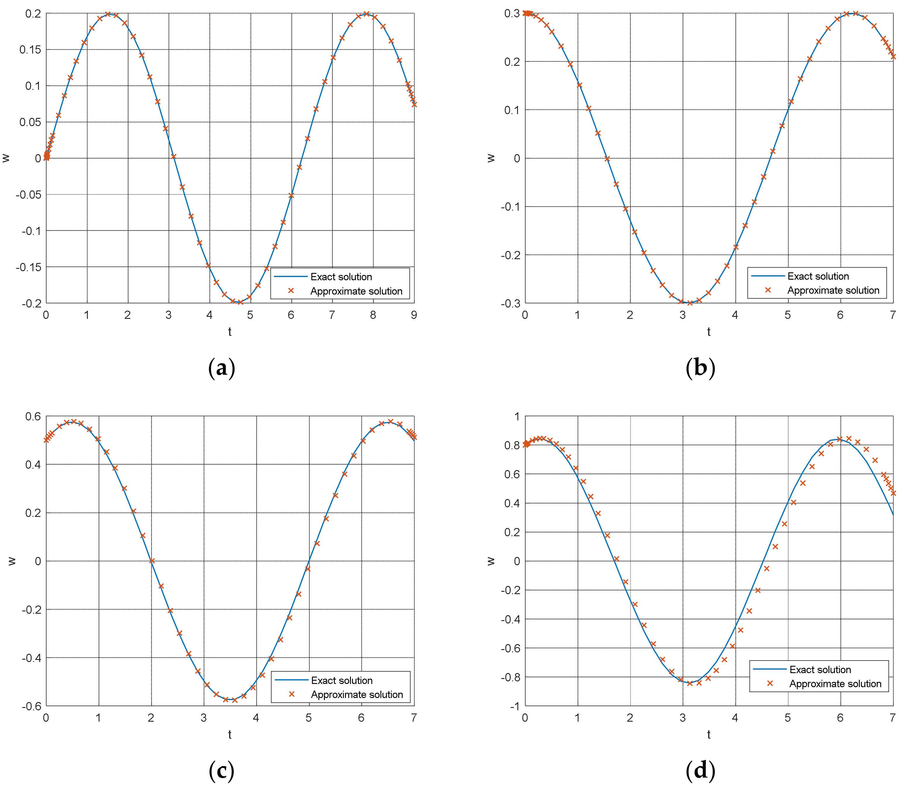
3. Tangent Oscillator

The tangent oscillator [3] is

$$w^{″}+{\omega }_0^2\tan w=0,w(0)=a,w^{\prime }(0)=b$$

(5)

One can choose $N=\sqrt{3}/2$ in Equation (3). We have

$${\omega }^2=\frac{{\omega }_0^2\tan (\sqrt{3}A/2)}{\sqrt{3}A/2}$$

(6)

where A is given in Equation (4). For given parameters of ${\omega }_0$, a, and b, the frequency can be calculated easily from Equation (6). To obtain an explicit formulation, one can consider the case of A << 1. In that case, we have

$$\tan w\approx w+\frac{1}{3}{w}^3$$

(7)

Equation (6) becomes

$${\omega }^2=\frac{{\omega }_0^2\tan (\sqrt{3}A/2)}{\sqrt{3}A/2}={\omega }_0^2(1+\frac{1}{4}{A}^2)$$

(8)

In view of Equation (4), we can convert Equation (8) to the form

$${\omega }^2={\omega }_0^2\left[1+\frac{1}{4}(a^2+\frac{b^2}{{\omega }^2})\right]$$

(9)

or

$$4{\omega }^4-(4+a^2){\omega }_0^2{\omega }^2-b^2{\omega }_0^2=0$$

(10)

Solving $\omega$ from Equation (10) and ignoring the meaningless root gives

$$\omega =\sqrt{\frac{(4+a^2){\omega }_0^2+\sqrt{{(4+a^2)}^2{\omega }_0^4+16b^2{\omega }_0^2}}{8}}$$

(11)

The approximate solution reads

$$w=A\cos (\omega t+\phi )$$

(12)

where $\phi$ is determined by the initial conditions

$$\phi =\arctan (-\frac{b}{a\omega })$$

(13)

In order to reveal the accuracy of the approximate solution, we resolve the problem by the homotopy perturbation method [19]. For small amplitude, Equation (5) is approximated as

$$w^{″}+{\omega }_0^2(w+\frac{1}{3}{w}^3)=0,w(0)=a,w^{\prime }(0)=b$$

(14)

The homotopy equation is

$$x^{″}+{\omega }^{2}x+h\left[{\omega }_0^{2}x-{\omega }^{2}x+\frac{1}{3}{\omega }_0^2{x}^3\right]=0$$

(15)

where h is the homotopy parameter, $0\le h\le 1$. When h = 1, Equation (15) becomes Equation (14). We assume that the solution is written as

$$w=w_0+h{w}_1+h^2{w}_2+\cdots$$

(16)

Following the method’s standard steps, we have

$${w^{″}}_0+{\omega }^2{w}_0=0,w_0(0)=a,{w^{\prime }}_0(0)=b$$

(17)

$${w^{″}}_1{}_1+{\omega }^2{w}_1+{\omega }_0^2{w}_0-{\omega }^2{w}_0+\frac{1}{3}{\omega }_0^2{w}_0^3=0,w_1(0)=0,{w^{\prime }}_0(0)=0$$

(18)

Equation (17) is a linear differential equation; its solution is

$$w_0=A\cos (\omega t+\phi )$$

(19)

where A and $\phi$ are given, respectively, in Equations (4) and (13). Now Equation (18) is updated as

$${w^{″}}_1+{\omega }^2{w}_1+({\omega }_0^2-{\omega }^2)A\cos (\omega t+\phi )+\frac{1}{3}{\omega }_0^2{A}^3{\cos }^3(\omega t+\phi )=0$$

(20)

or

$${w^{″}}_1+{\omega }^2{w}_1+({\omega }_0^2-{\omega }^2+\frac{1}{4}{\omega }_0^2{A}^2)A\cos (\omega t+\phi )+\frac{1}{12}{\omega }_0^2{A}^3\cos (3\omega t+3\phi )=0$$

(21)

The solution of Equation (21) is

$$w_1=-\frac{1}{2\omega }({\omega }_0^2-{\omega }^2+\frac{1}{4}{\omega }_0^2{A}^2)At\sin (\omega t+\phi )+\frac{1}{96{\omega }^2}{\omega }_0^2{A}^3\cos (3\omega t+3\phi )+C$$

(22)

where C is an integral constant. In Equation (22), the term of $t\sin (\omega t+\phi )$ is not periodic when t tends to infinity, so its coefficient has to be zero to have a periodic solution, that is

$${\omega }_0^2-{\omega }^2+\frac{1}{4}{\omega }_0^2{A}^2=0$$

(23)

or

$$\omega ={\omega }_0^{}\sqrt{1+\frac{1}{4}{A}^2}$$

(24)

This result can also be obtained by the multiple scales method [24], and it is exactly the same as that given in Equation (9). Considering the initial conditions, $w_1(0)=0,{w^{\prime }}_0(0)=0$, Equation (22) becomes

$$w_1=\frac{1}{96{\omega }^2}{\omega }_0^2{A}^3\left[\cos (3\omega t+3\phi )-\cos (\omega t+\phi )\right]$$

(25)

The first-order approximate solution is obtained by setting h = 1 in Equation (16), that is

$$w=w_0+w_1=A\cos (\omega t+\phi )+\frac{1}{96{\omega }^2}{\omega }_0^2{A}^3\left[\cos (3\omega t+3\phi )-\cos (\omega t+\phi )\right]$$

(26)

Comparison of the approximate solution, $w=A\cos (\omega t+\phi )$, with $\omega$ given in Equation (11), with the exact solution for various cases is illustrated in Figure 1, where ${\omega }_0=1$.

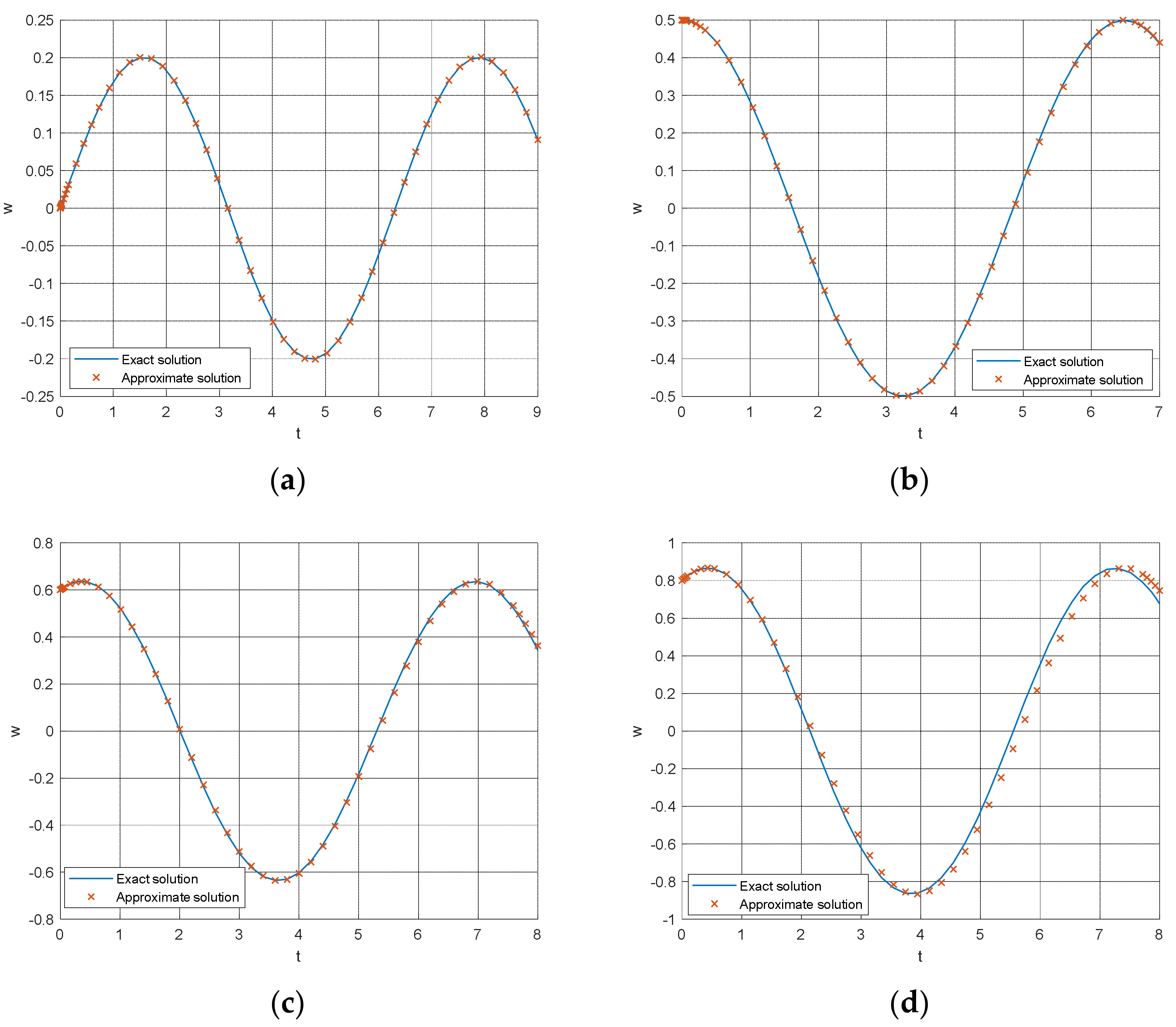
4. Hyperbolic Tangent Oscillator

The hyperbolic tangent oscillator reads [1]

$$w^{″}+{\omega }_0^2\tanh w=0,w(0)=a,w^{\prime }(0)=b$$

(27)

We can immediately obtain the following frequency–amplitude relation:

$${\omega }^2=\frac{{\omega }_0^2\tanh (\sqrt{3}A/2)}{\sqrt{3}A/2}$$

(28)

where A is defined in Equation (4).

For small amplitude, tanh w can be approximated as

$$\tanh w\approx w-\frac{1}{3}{w}^3$$

(29)

Equation (28) becomes:

$${\omega }^2=\frac{{\omega }_0^2\tanh (\sqrt{3}A/2)}{\sqrt{3}A/2}={\omega }_0^2(1-\frac{1}{4}{A}^2)$$

(30)

In view of Equation (4), Equation (30) turns out to be

$${\omega }^2={\omega }_0^2\left[1-\frac{1}{4}(a^2+\frac{b^2}{{\omega }^2})\right]$$

(31)

or

$$4{\omega }^4-(4-a^2){\omega }_0^2{\omega }^2+b^2{\omega }_0^2=0$$

(32)

Solving $\omega$ from Equation (32) and ignoring the meaningless root gives

$$\omega =\sqrt{\frac{(4-a^2){\omega }_0^2+\sqrt{{(4-a^2)}^2{\omega }_0^4-16b^2{\omega }_0^2}}{8}}$$

(33)

This is the same as that obtained by the homotopy perturbation method [1]. Comparison of the approximate solution with the exact solution for various cases is illustrated in Figure 2, where ${\omega }_0=1$.

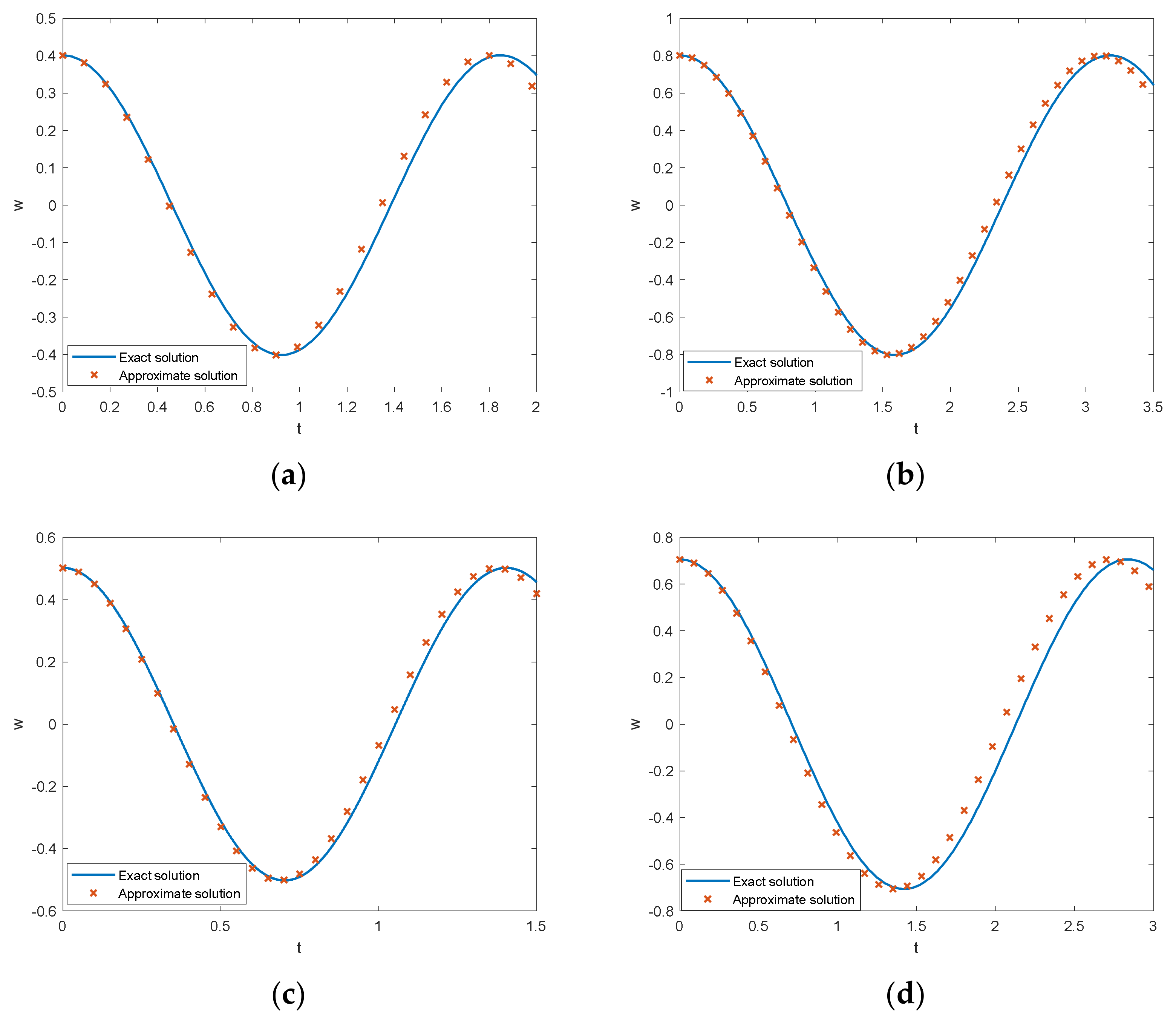
5. Singular Oscillator

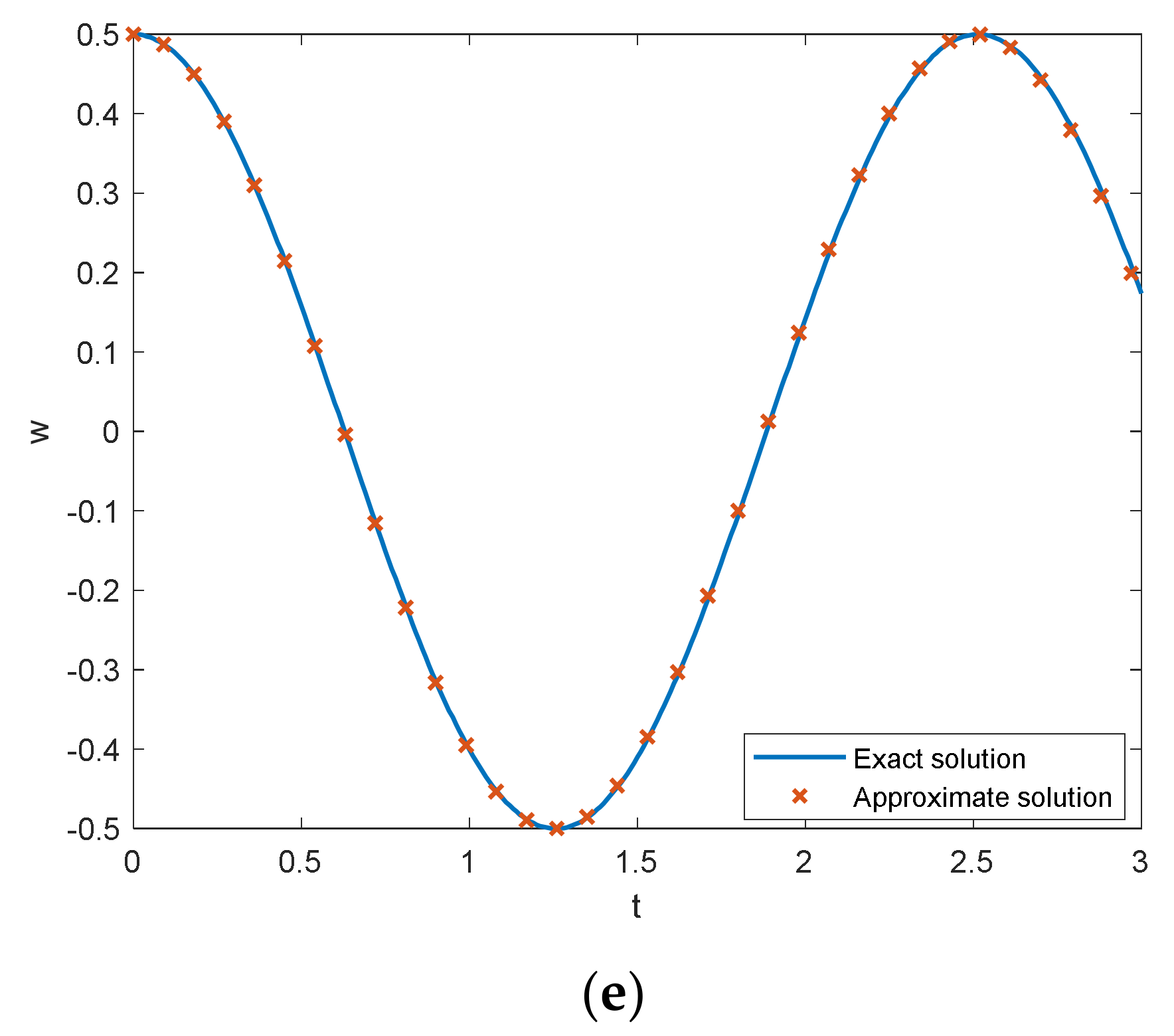
Now we consider a singular oscillator [9]

$$w^{″}+\frac{1}{kw}=0,w(0)=a,w^{\prime }(0)=b$$

(34)

For the singular oscillator, we choose N = 0.8 [20], that is

$${\omega }^2={\left.\frac{1}{k{w}^2}\right|}_{w=NA}=\frac{1}{k{N}^2{A}^2}=\frac{1}{k{N}^2(a^2+\frac{b^2}{{\omega }^2})}$$

(35)

Simplifying Equation (35) gives

$$k{N}^2(a^2{\omega }^2+b^2)=1$$

(36)

Solving $\omega$ from Equation (36) leads to the result

$$\omega =\frac{1}{a}\sqrt{\frac{1}{k{N}^2}-b^2}$$

(37)

When b = 0 and N = 0.8, we have

$$\omega =\frac{1}{a}\sqrt{\frac{1}{k{N}^2}}=1.25k^{-1/2}{a}^{-1}$$

(38)

The exact frequency for b = 0 is [9]

$${\omega }_{\mathrm{exact}}=1.2533k^{-1/2}{a}^{-1}$$

(39)

The relative error is 0.26%. Figure 3 illustrates the accuracy of the approximate solution.

6. MEMS Oscillator

The fast development of nanotechnology and material science have led to skyrocketing interest in MEMS systems for the last decade [30,31,32]. We consider the following MEMS oscillator [33]

$$y^{″}+y-\frac{b}{1-y}=0,y(0)=0,y^{\prime }(0)=0$$

(40)

where y is the dimensionless displacement, y < 1, and b is constant.

In order to use the above frequency formulation, we introduce a transformation:

$$y=A-x$$

(41)

where A is the amplitude, Equation (40) becomes

$$x^{″}+x+\frac{b}{1-A+x}-A=0$$

(42)

where f(x) is the restoring force,

$$f(x)=x+\frac{b}{1-A+x}-A$$

(43)

It requires f(0) = 0, that is

$$\frac{b}{1-A}=A$$

(44)

or

$$A=\frac{1-\sqrt{1-4b}}{2}$$

(45)

In view of Equation (44), we can rewrite Equation (43) in the form

$$f(x)=x-\frac{bx}{(1-A)(1-A+x)}$$

(46)

$${\omega }^2={\left.\frac{f(x)}{x}\right|}_{x=-0.8A}$$

(47)

This leads to the following formulation

$${\omega }^2=1-\frac{b}{(1-A)(1-A-0.8A)}$$

(48)

Solving $\omega$ from Equation (48), we obtain

$$\omega =\sqrt{\frac{1-5.6b+\sqrt{1-4b}}{1-3.6b+\sqrt{1-4b}}}$$

(49)

Finally, we obtain the following approximate periodic solution:

$$x(t)=A\cos (\omega t)$$

(50)

By the inverse transformation of Equation (41), we obtain

$$y(t)=A(1-\cos (\omega t))=2A{\sin }^2(\frac{\omega }{2}t)$$

(51)

where $\omega$ is given in Equation (49). Figure 4 shows a high accuracy of Equation (51) when b < 0.15.

7. Conclusions

He’s frequency formulation could be extended to fractal oscillators [34] as well as non-conservative oscillators [35,36,37]. In engineering, a simple calculation is always appreciated; the simpler the calculation, the better. This paper proposes possibly the simplest method for quickly inspecting the frequency property of a nonlinear oscillator; the one-step solution yields a highly accurate result, which is quite palatable.

References

1. Song, H.Y. A modification of homotopy perturbation method for a hyperbolic tangent oscillator arising in nonlinear packaging system. J. Low Freq. Noise Vib. Active Control 2019, 38, 914–917. [Google Scholar] [CrossRef] [Green Version]
2. Song, H.Y. A thermodynamics model for a packing dynamical system. Therm. Sci. 2020, 24, 2331–2335. [Google Scholar] [CrossRef]
3. Kuang, W.; Wang, J.; Huang, C.; Lu, L.; Gao, D.; Wang, Z.; Ge, C. Homotopy perturbation method with an auxiliary term for the optimal design of a tangent nonlinear packaging system. J. Low Freq. Noise Vib. Active Control 2019, 38, 1075–1080. [Google Scholar] [CrossRef]
4. Ji, Q.P.; Wang, J.; Lu, L.X.; Ge, C.F. Li-He’s modified homotopy perturbation method coupled with the energy method for the dropping shock response of a tangent nonlinear packaging system. J. Low Freq. Noise Vib. Active Control 2021, 40, 675–682. [Google Scholar] [CrossRef]
5. Clementi, F.; Gazzani, V.; Poiani, M.; Lenci, S. Assessment of seismic behaviour of heritage masonry buildings using numerical modelling. J. Build. Eng. 2016, 8, 29–47. [Google Scholar] [CrossRef]
6. Dertimanis, V.K.; Chatzi, E.N.; Masri, S.F. On the Active Vibration Control of Nonlinear Uncertain Structures. J. Appl. Comp. Mech. 2021, 7, 1183–1197. [Google Scholar]
7. El-Dib, Y.O.; Matoog, R.T. The Rank Upgrading Technique for a Harmonic Restoring Force of Nonlinear Oscillators. J. Appl. Comp. Mech. 2021, 7, 782–789. [Google Scholar]
8. Anjum, N.; He, J.H.; Ain, Q.T.; Tian, D. Li-He’s modified homotopy perturbation method for doubly-clamped electrically actuated microbeams-based microelectromechanical system. Facta Univ. Mech. Eng. 2021. [Google Scholar] [CrossRef]
9. Nawaz, Y.; Arif, M.S.; Bibi, M.; Naz, M.; Fayyaz, R. An effective modification of He’s variational approach to a nonlinear oscillator. J. Low Freq. Noise Vib. Active Control 2019, 38, 1013–1022. [Google Scholar] [CrossRef]
10. Ganji, D.D.; Gorji, M.; Soleimani, S.; Esmaeilpour, M. Solution of nonlinear cubic-quintic Duffing oscillators using He’s Energy Balance Method. J. Zhejiang Univ.-Sci. A 2009, 10, 1263–1268. [Google Scholar] [CrossRef]
11. Ganji, S.S.; Barari, A.; Karimpour, S.; Domairry, G. Motion of a rigid rod rocking back and forth and cubic-quitic Duffing oscillators. J. Theor. Appl. Mech. 2012, 50, 215–229. [Google Scholar]
12. Beléndez, A.; Beléndez, T.; Martínez, F.J.; Pascual, C.; Alvarez, M.L.; Arribas, E. Exact solution for the unforced Duffing oscillator with cubic and quintic nonlinearities. Nonlinear Dyn. 2016, 86, 1687–1700. [Google Scholar] [CrossRef] [Green Version]
13. Suleman, M.; Wu, Q.B. Comparative Solution of Nonlinear Quintic Cubic Oscillator Using Modified Homotopy Perturbation Method. Adv. Math. Phys. 2015, 932905. [Google Scholar] [CrossRef]
14. Razzak, M.A. An analytical approximate technique for solving cubic-quintic Duffing oscillator. Alex. Eng. J. 2016, 55, 2959–2965. [Google Scholar] [CrossRef] [Green Version]
15. Wang, K.J.; Wang, G.D. Gamma function method for the nonlinear cubic-quintic Duffing oscillators. J. Low Freq. Noise Vib. Active Control 2021. [Google Scholar] [CrossRef]
16. Wang, K.J. On new abundant exact traveling wave solutions to the local fractional Gardner equation defined on Cantor sets. Math. Methods Appl. Sci. 2021. [Google Scholar] [CrossRef]
17. Wang, K.J. Generalized variational principle and periodic wave solution to the modified equal width-Burgers equation in nonlinear dispersion media. Phys. Lett. A 2021, 419, 127723. [Google Scholar] [CrossRef]
18. Wang, K.J.; Zhang, P.L. Investigation of the periodic solution of the time-space fractional Sasa-Satsuma equation arising in the monomode optical fibers. EPL 2021. [Google Scholar] [CrossRef]
19. He, J.H. The simpler, the better: Analytical methods for nonlinear oscillators and fractional oscillators. J. Low Freq. Noise Vib. Active Control 2019, 38, 1252–1260. [Google Scholar] [CrossRef] [Green Version]
20. Qie, N.; Hou, W.F.; He, J.H. The fastest insight into the large amplitude vibration of a string. Rep. Mechan. Eng. 2020, 2, 1–5. [Google Scholar] [CrossRef]
21. Feng, G.Q. He’s frequency formula to fractal undamped Duffing equation. J. Low Freq. Noise Vib. Active Control 2021. [Google Scholar] [CrossRef]
22. Liu, C.X. A short remark on He’s frequency formulation. J. Low Freq. Noise Vib. Active Control 2021, 40, 672–674. [Google Scholar] [CrossRef]
23. Liu, C.X. Periodic solution of fractal Phi-4 equation. Therm. Sci. 2021, 25, 1345–1350. [Google Scholar] [CrossRef]
24. Elías-Zúñiga, A.; Palacios-Pineda, L.M.; Jiménez-Cedeño, I.H.; Martínez-Romero, O.; Trejo, D.O. He’s frequency-amplitude formulation for nonlinear oscillators using Jacobi elliptic functions. J. Low Freq. Noise Vib. Active Control 2020, 39, 1216–1223. [Google Scholar] [CrossRef]
25. Elías-Zúñiga, A.; Palacios-Pineda, L.M.; Jiménez-Cedeño, I.H.; Martínez-Romero, O.; Olvera-Trejo, D. Enhanced He’s frequency-amplitude formulation for nonlinear oscillators. Results Phys. 2020, 19, 103626. [Google Scholar] [CrossRef]
26. Wu, Y.; Liu, Y.P. Residual calculation in He’s frequency-amplitude formulation. J. Low Freq. Noise Vib. Active Control 2021, 40, 1040–1047. [Google Scholar] [CrossRef] [Green Version]
27. Zuo, Y.T. A gecko-like fractal receptor of a three-dimensional printing technology: A fractal oscillator. J. Math. Chem. 2021, 59, 735–744. [Google Scholar] [CrossRef]
28. He, C.H. An introduction to an ancient Chinese algorithm and its modification. Int. J. Numer. Methods Heat Fluid Flow 2016, 26, 2486–2491. [Google Scholar] [CrossRef]
29. Khan, W.A. Numerical simulation of Chun-Hui He’s iteration method with applications in engineering. Int. J. Numer. Methods Heat Fluid Flow 2021. [Google Scholar] [CrossRef]
30. Sedighi, H.M.; Shirazi, K.H.; Attarzadeh, M.A. A study on the quintic nonlinear beam vibrations using asymptotic approximate approaches. Acta Astronaut. 2013, 91, 245–250. [Google Scholar] [CrossRef]
31. Sedighi, H.M. Size-dependent dynamic pull-in instability of vibrating electrically actuated microbeams based on the strain gradient elasticity theory. Acta Astronaut. 2014, 95, 111–123. [Google Scholar] [CrossRef]
32. Sedighi, H.M.; Keivani, M.; Abadyan, M. Modified continuum model for stability analysis of asymmetric FGM double-sided NEMS: Corrections due to finite conductivity, surface energy and nonlocal effect. Comp. Part B-Eng. 2015, 83, 117–133. [Google Scholar] [CrossRef]
33. Zhang, Y.N.; Tian, D.; Pang, J. A fast estimation of the frequency property of the microelectromechanical system oscillator. J. Low Freq. Noise Vib. Active Control 2021. [Google Scholar] [CrossRef]
34. Wang, K.L.; Wei, C.F. A powerful and simple frequency formula to nonlinear fractal oscillators. J. Low Freq. Noise Vib. Active Control. 2021, 40, 1373–1379. [Google Scholar] [CrossRef]
35. El-Dib, Y.O. The frequency estimation for non-conservative nonlinear oscillation. ZAMM-Z. Angew. Math. Mech. 2021. [Google Scholar] [CrossRef]
36. Wang, K.J. A fast insight into the nonlinear oscillation of nano-electro mechanical resonators considering the size effect and the van der Waals force. EPL Lett. J. Explor. Front. Phys. 2021. [Google Scholar] [CrossRef]
37. Popov, M. Friction under Large-Amplitude Normal Oscillations. Facta Univ. Ser. Mech. Eng. 2021, 19, 105–113. [Google Scholar] [CrossRef]
Figure 1. The approximate solution of Equation (12) vs. the exact one of Equation (5). (a) (a,b) = (0, 0.2); (b) (a,b) = (0.3, 0); (c) (a,b) = (0.5, 0.3); and (d) (a,b) = (0.8, 0.3).
Axioms 10 00320 g001
Figure 2. The approximate solution ( w = A cos ( ω t + φ ) ) vs. the exact one of Equation (27). (a) (a,b) = (0, 0.2); (b) (a,b) = (0.5, 0); (c) (a,b) = (0.6, 0.2); and (d) (a,b) = (0.8, 0.3).
Axioms 10 00320 g002
Figure 3. The comparison of approximate solution w = A cos ( ω t + φ ) with exact one of Equation (34). (a) (k,a,b) = (0.8, 0.4, 0.1); (b) (k,a,b) = (0.6, 0.8, 0.1); (c) (k,a,b) = (0.3, 0.5, 0.2); (d) (k,a,b) = (0.6, 0.7, 0.2); and (e) (k,a,b) = (1, 0.5, 0).
Axioms 10 00320 g003aAxioms 10 00320 g003b
Figure 4. The MEMS oscillator with different values of b. (a) b = 0.05; (b) b = 0.10; and (c) b = 0.15.
Axioms 10 00320 g004
Publisher’s Note: MDPI stays neutral with regard to jurisdictional claims in published maps and institutional affiliations.