1. Introduction
The Marshall–Olkin family of distributions was introduced by [
1]. This is an interesting endeavour for associating additional parameter to an existing baseline. The resulting new probability distributions provide more flexibility to model various kinds of data. The early studies of the this scheme by [
2,
3,
4,
5,
6,
7,
8], etc. offered its features. For a comprehensive discussion, one can refer a write-up by [
9]. Keeping in view its applications, researchers focused on generalizations and extensions of the Marshall–Olkinn family of distribution. For example, exponentiated Marshall–Olkin extended family [
10], Harris extended family [
11], truncated negative-binomial generalized Marshall–Olkin family [
12], beta Marshall–Olkin family [
13], Kumaraswamy Marshall–Olkin family [
14], truncated discrete Mittag–Leffler family [
15], Marshall–Olkin generalized family [
16], truncated discrete Linnik family [
17], etc.
Recently, ref. [
18] proposed a new family of distributions called the Weibull Marshall–Olkin generalized family. Its cumulative distribution function (cdf) with arbitrary baseline
, is given by
and
. This family is derived based on T-X family introduced by [
19].
In many practical situations, discretizing statistical models from existing continuous distributions brings a crucial role. Consequently, some discrete distributions derived based on popular continuous models, for example, see, refs. [
20,
21,
22,
23,
24,
25], etc. Furthermore, several discrete distributions appeared in the literature by using continuous Marshall–Olkin distributions [
26,
27,
28].
The most prominent motivating factor that pushed us towards the introduction of this new discrete distribution is the that while comparing with the volume of literature in continuous case, only limited research works have been inscribed about the discrete version of continuous family of distributions. The properties of the proposed model itself is another source of motivation. That is, the proposed new discrete model has positively skewed, decreasing and symmetric probability mass function (pmf). Moreover, the new distribution has decreasing, increasing, unimodal and bathtub shaped hazard rate functions (hrf). In addition to this, we offered a comparison of the estimation methods and real-life data application to explain how well the proposed model give consistently better fit than the other well-known discrete distributions.
The rest of the paper is outlined as follows: In
Section 2, we propose a new discrete family of distributions and a special case of the derived family together with its probabilistic properties. Two distinct estimation procedures for parameters estimation are illustrated in
Section 3. In
Section 4, we give demonstration of the two different methods for constructing confidence intervals for the proposed distribution.
Section 5 inculcates the Monte Carlo simulations study. Applications to the two real data sets to illustrate the performance of the new family are explained in
Section 6.
Section 7 offers some concluding remarks.
2. Discrete Weibull Marshall–Olkin Exponential Distribution
In this section, we propose a new discrete family of distributions namely discrete Weibull Marshall–Olkin family of distributions. Different methods and constructions of discrete analogs of continuous distributions are given in [
29]. If the underlying continuous life time
X has the survival function
, the pmf of the discrete random variable associated with that continuous distribution can be written as
The new family is generated by discretizing the continuous survival in Equation (
1) using Equation (
2), we obtain new family of discrete distribution with the pmf
. The pmf can be written as
The survival function of the discrete random variable having the pmf (
3) is given by
We study a special case of this family, namely, discrete Weibull Marshall–Olkin exponential (DWMOE) distribution. The exponential distribution was chosen because it is the most tractable model. In practice for modeling and analyzing of random phenomenons, other distributions could be used.
Let the parent distribution be exponential with parameter
and survival function
. We set
and
. Then, the pmf of the new model using (
3) is given by
We called this new distribution the DWMOE distribution with parameters
,
b and
. Note that, when
, the distribution with pmf (
5) reduces to discrete Marshall–Olkin distributions, when
and
, (
5) becomes geometric distribution. The corresponding cumulative distribution function (cdf) corresponding to (
5) can be written as
The corresponding hrf is given by
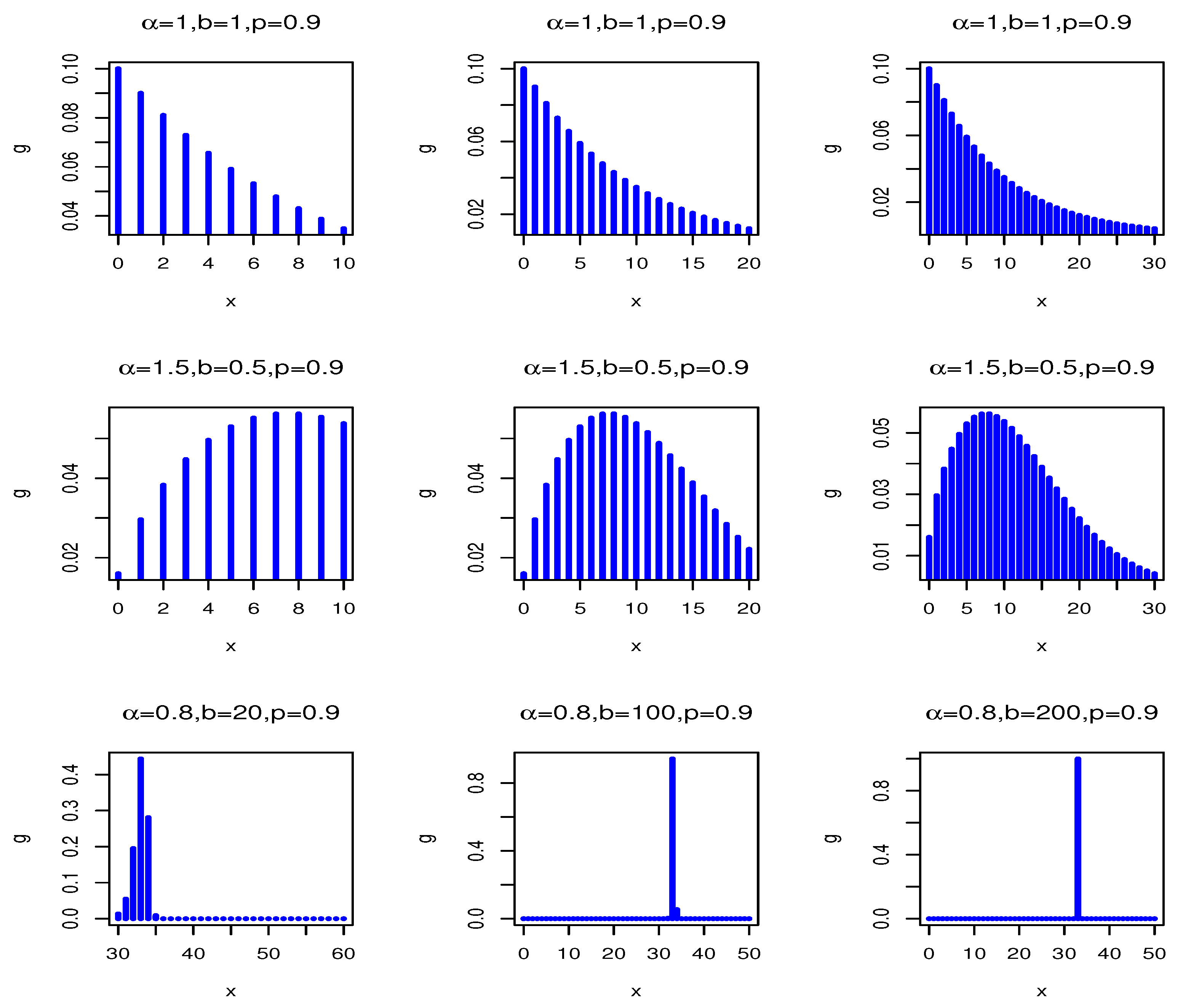
Figure 1 shows the plots of the pmf of the DWMOE distribution for various values of
,
b and
. The pmf can be decreasing and upside-down bathtub shaped. Furthermore,
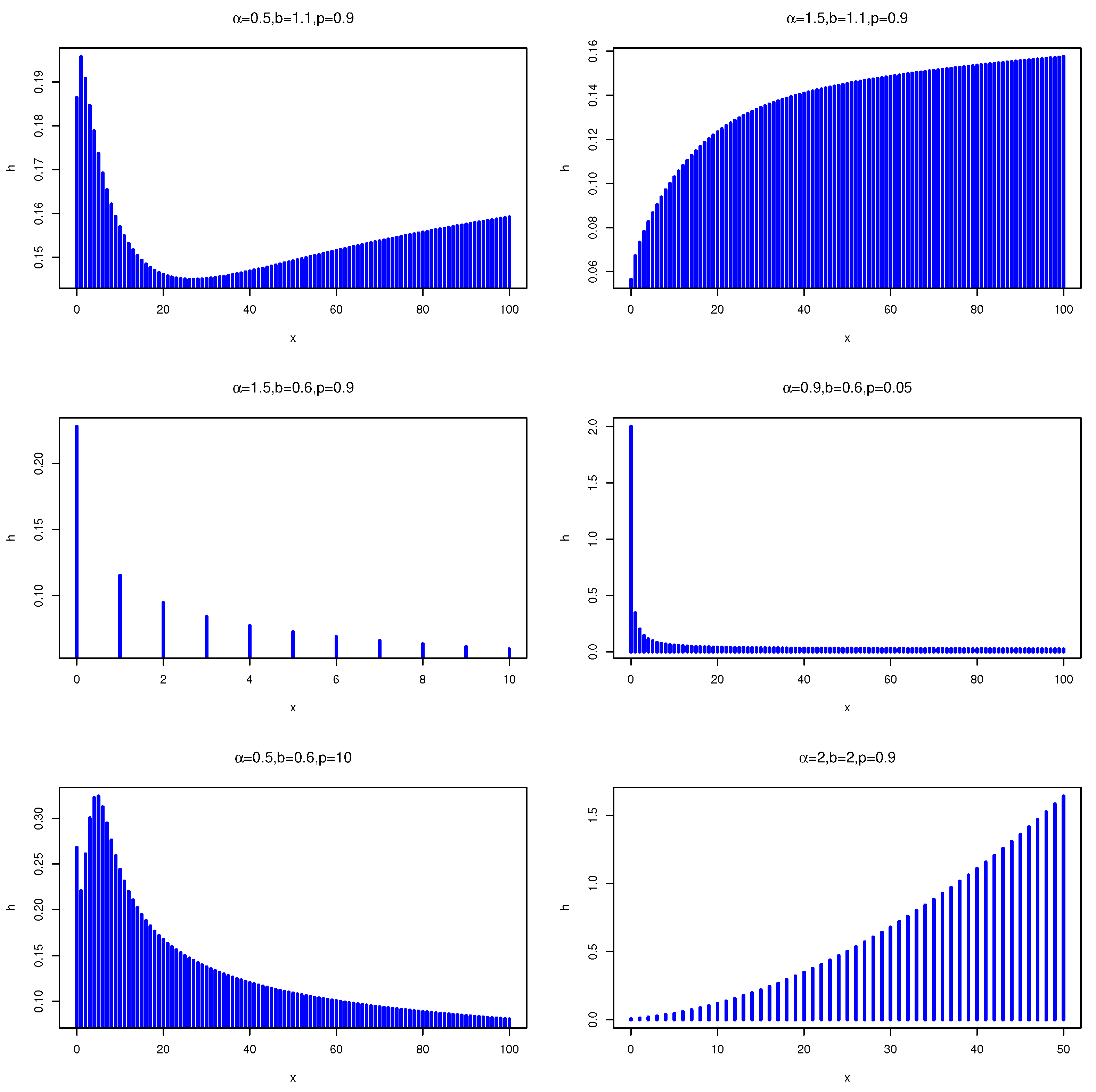
Figure 2 illustrates some of the possible shapes of the hrf of DWMOE distribution for selected values of the parameters. From figures, we can see that the hrf can be increasing, decreasing, bathtub, and upside-down bathtub shaped. Therefore, the DWMOE distribution is very efficient for modeling various data sets.
2.1. General Characteristics of the DWMOE Distribution
In this section, we study some general properties of the DWMOE distribution.
2.1.1. Quantiles, Probability Generating Function, Mean and Variance
Suppose
X follows the DWMOE with cdf
. The quantile function
,
of DWMOE is given as
where
u follows uniform distribution with support (0,1). Equation (
7) can be used to simulate the DWMOE random variable. First, simulate a random variable
u and compute the value of
X in (
7), which is not necessarily an integer. The DWMOE random variate
X is the largest integer
, denoted as
.
In particular, the Median
M is given as
The probability generating function (pgf) of the DWMOE(
,
b,
) distribution is given by
The mean and variance do not have compact forms, but still the solutions of following equation gives mean and variance of random variable having DWMOE(
,
b,
) model.
and
Using statistical software, the mean and variance of the DWMOE(
,
b,
) distribution for different values of
,
b and
are calculated in
Table 1. From this, we can say that the mean increases with
and
for different values of
b. Moreover, depending on the values of
and
, the mean of the distribution can be smaller or greater than its variance. Therefore, the parameters of the DWMOE(
,
b,
) distribution can be used to model different data sets.
2.1.2. Shannon Entropy
In probabilistic context, Shannon entropy is a measure of variation of the uncertainty, with higher entropy corresponding to less information. For a discrete random variable
X with pmf
g(
x), the Shannon entropy is defined as
Combining (
8) and (
5) gives
Consider the another representation of pmf of DWMOE, that is after rearranging the pmf of DWMOE, we get
Note that when and then . This indicates that smaller values of b increase the uncertainty in the distribution.
3. Estimation Methods
To acquire the unknown model parameters, we will look at two estimation methods in this section. Maximum likelihood estimation (MLE) and the Bayesian estimation method are the two methods.
3.1. MLE Method
Let
a random sample of size
n from the DWMOE distribution and
its observed values. The log-likelihood equation of the vector
are given by
The non-linear likelihood equations are obtained by differentiating Equation (
10) with respect to the parameters
, and
, respectively:
and
Equating (
11)–(
13) with zeros and solving simultaneously by using iterative methods such as Newton–Raphson, we obtain the MLEs of
, and
. The asymptotic inference for the parameter vector
can be based on the normal approximation of the MLE of
. Indeed, under some regular conditions stated in [
30], we have
is approximately normally distributed with mean
and asymptotic variance-covariance matrix
.
3.2. Bayesian Estimation Model
We explore the Square error type of loss function in Bayesian estimation. Several authors discussed this loss function based on various models [
31,
32]. Moreover, several authors discussed Bayesian estimation for parameters of the discrete distribution. For example, see [
33,
34,
35], etc. For the Bayesian analysis, the prior distributions for each parameter of DWMOE distribution are essential. When prior information about the parameters is lacking, the Bayesian study might use the non-informative prior. Most previous studies of Weibull and Marshall–Olkin family distributions have Gamma prior distribution. Therefore, we supposed the informative priors for parameters
and
b. The independent gamma distribution is our prior distribution of choice since it plays a significant role in estimating the parameters. While the parameter
, we used Jeffreys’ rule.
The independent joint prior density function of
can be written as follows:
The prior distribution of
may be considered to be
The joint prior density function of
can be written as follows:
From the likelihood function and joint prior function (
16), the joint posterior density function of
is obtained. The joint posterior of the DWMOE distribution can be written as
Using the most common loss function (symmetric), which is a squared error. Bayesian estimators of
based on the squared error loss function are defined by Markov Chain Monte Carlo (MCMC).
As the integrals given by (
18) cannot be estimated directly. Because of this, we used the MCMC to find an approximate value of integrals. A significant sub-class of the MCMC techniques is the Gibbs sampling and more general Metropolis within Gibbs samplers. The Metropolis-Hastings (MH) bound with the Gibbs sampling were the two most common instances of the MCMC method. Because of the similarity of the MH algorithm with acceptance-rejection sampling, each iteration of the algorithm produces a corresponding candidate value from the proposal distribution. We used the MH within the Gibbs sampling steps to produce random samples of conditional posterior densities from the DWMOE distribution family:
and
4. Confidence Intervals
In this section, we propose two different methods to construct confidence intervals (CI) for the unknown parameters of the DWMOE distribution, which are asymptotic confidence interval (ACI) in MLE and credible confidence interval in MCMC of , and .
4.1. Asymptotic Confidence Intervals
The most common method to set confidence bounds for the parameters is to use the asymptotic normal distribution of the MLE. In relation to the asymptotic variance-covariance matrix of the MLE of the parameters, Fisher information matrix
, where it is composed of the negative second derivatives of the natural logarithm of the likelihood function evaluated at
Suppose the asymptotic variance-covariance matrix of the parameter vector
is
where
.
A
confidence interval for parameter
can be constructed based on the asymptotic normality of the MLE.
where
is the percentile of the standard normal distribution with right tail probability
.
4.2. Highest Posterior Density
The Highest Posterior Density (HPD) Intervals: [
36] discussed this technique to generate the HPD intervals of unknown parameters of the benefit distribution. In this study, samples drawn with the proposed MH algorithm should be used to generate time-lapse estimates. From the percentile tail points, for instance, a
HPD interval can be obtained with two points for
parameters of DWMOE distribution from the MCMC sampling outputs. It is sometimes useful to present the posterior median to informally check on possible asymmetry in the posterior density of a parameter.
According to [
36], the BCIs of the parameters of DWMOE distribution
can be obtained through the following steps:
- 1.
Arrange as , and , where M denotes the length of the generated of MH algorithm.
- 2.
The symmetric credible intervals of are obtained as: , and .
5. Simulation
In order to compare the classical estimation methods, the Monte-Carlo simulation procedure is carried out: MLE, and Bayesian estimation method under square error loss function based on MCMC, for estimation of DWMOE lifetime distribution parameters by R program. Monte-Carlo experiments are performed based on t data generated on 10,000 random DWMOE distribution samples using Equation (
7), where
x has DWMOE lifetime for various parameter actual values as:
Case 1: with different .
Case 2: with different .
Case 3: with different .
and different sample sizes and . We could describe the best methods of estimators as minimizing estimators’ Bias, mean squared error (MSE) and confidence interval when .
The simulation results of the methods presented in this paper for point estimation are summarized in the
Table 2,
Table 3 and
Table 4. We consider the Bias, MSE, lower and upper of confidence interval values in order to perform the required comparison between various point estimation methods. The following remarks can be noted from these tables:
- 1.
For fixed actual parameters of DWMOE distribution, the Bias, and MSE decrease as n increases.
- 2.
When increases, the Bias and MSE for all parameters decrease.
- 3.
When b increases, the Bias and MSE for and parameters decrease.
- 4.
Bayesian estimation is the best estimation method according Bias and MSE.
- 5.
The confidence interval of Bayesian estimation is shorter confidence interval than MLE ACI for parameters of DWMOE distribution.
6. Applications
In this section, we illustrate the usefulness of the newly proposed DWMOE distribution. We fit the DWMOE distribution to two data sets and compare the results with those of the fitted Kumaraswamy-geometric (KG), discrete Lindley (DL), and geometric models. For comparing the these distributions, we estimated the values of unknown parameters by the maximum likelihood method with standard errors (SE). Moreover, the fitted distributions are compared using the −log likelihood (−logL), AIC (Akaike Information Criterion), BIC (Bayesian Information Criterion), Kolmogorov–Smirnov (K-S) statistic, the corresponding p-values, the values of Anderson-Darling () and Cramér von Mises (). The considered data sets are presented below.
Data set 1: The first dataset represents COVID-19 data belong to Australia of 32 days, which are recorded from 3 September to 4 October 2020, see, ref. [
37]. The data set is:
| 6 15 59 11 5 9 8 11 7 9 6 7 6 0 8 8 5 7 5 2 35 2 8 1 2
3 7 4 2 2 3 |
Data set 2: The second data set refers the integer part of the lifetime of fifty devices in weeks is given by [
38]. The data set is:
| 0 0 1 1 1 1 1 2 3 6 7 11 12 18 18 18 18 18 21 32 36 40 45 46 47 50 55 |
| 60 63 63 67 67 67 67 72 75 79 82 82 83 84 84 84 85 85 85 85 85 86 86 |
Table 5 and
Table 6 represent the values of descriptive study for the fitted DWMOE, KG, DL and geometric models for Data set 1 and Data set 2, respectively. From the study, the smallest −logL, AIC, BIC, K-S statistic,
,
and the highest
p-values are obtained for the DWMOE distribution. From these results, the new DWMOE distribution is the adequate model than others. Therefore, it can be used for fitting these data sets.
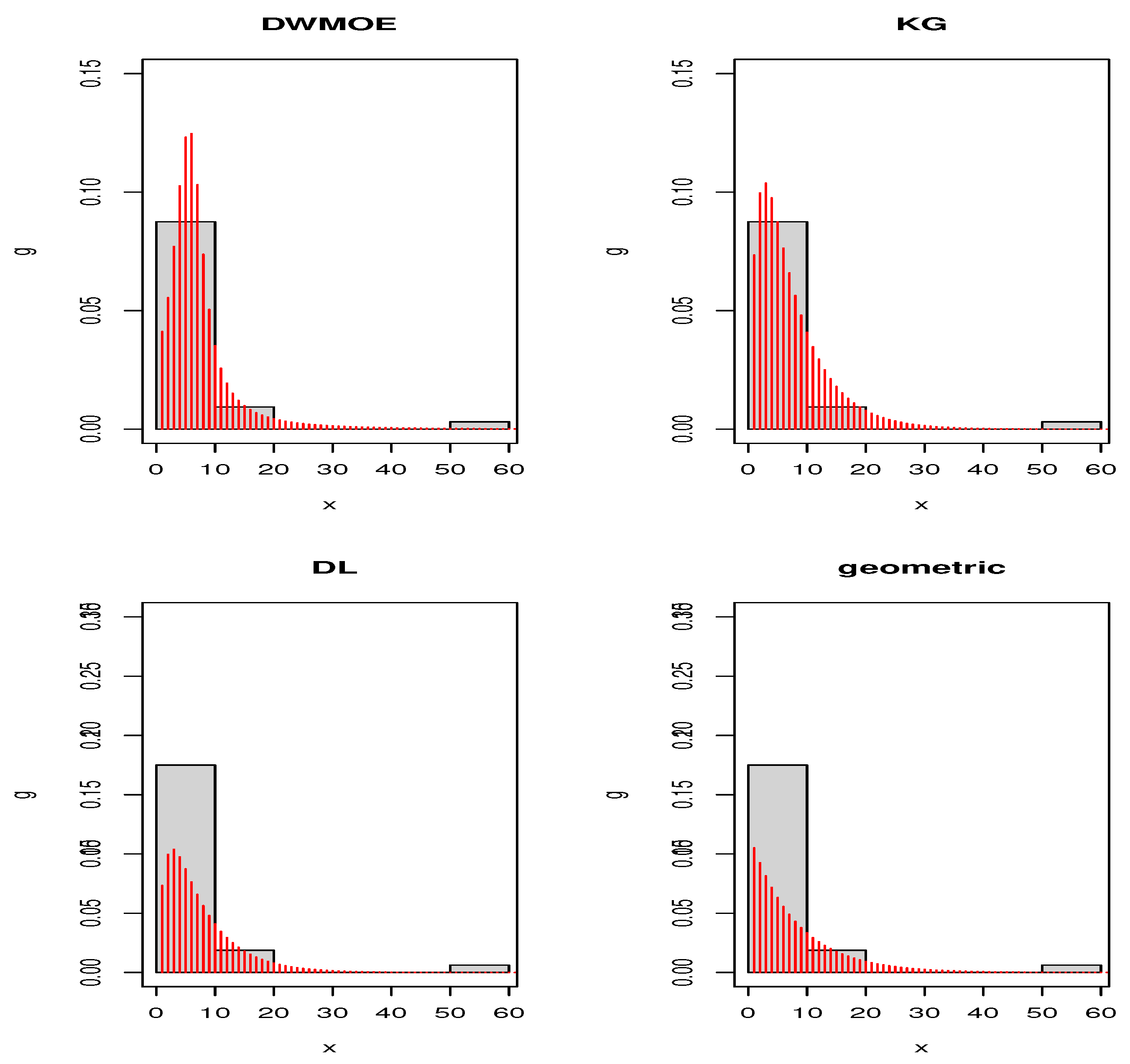
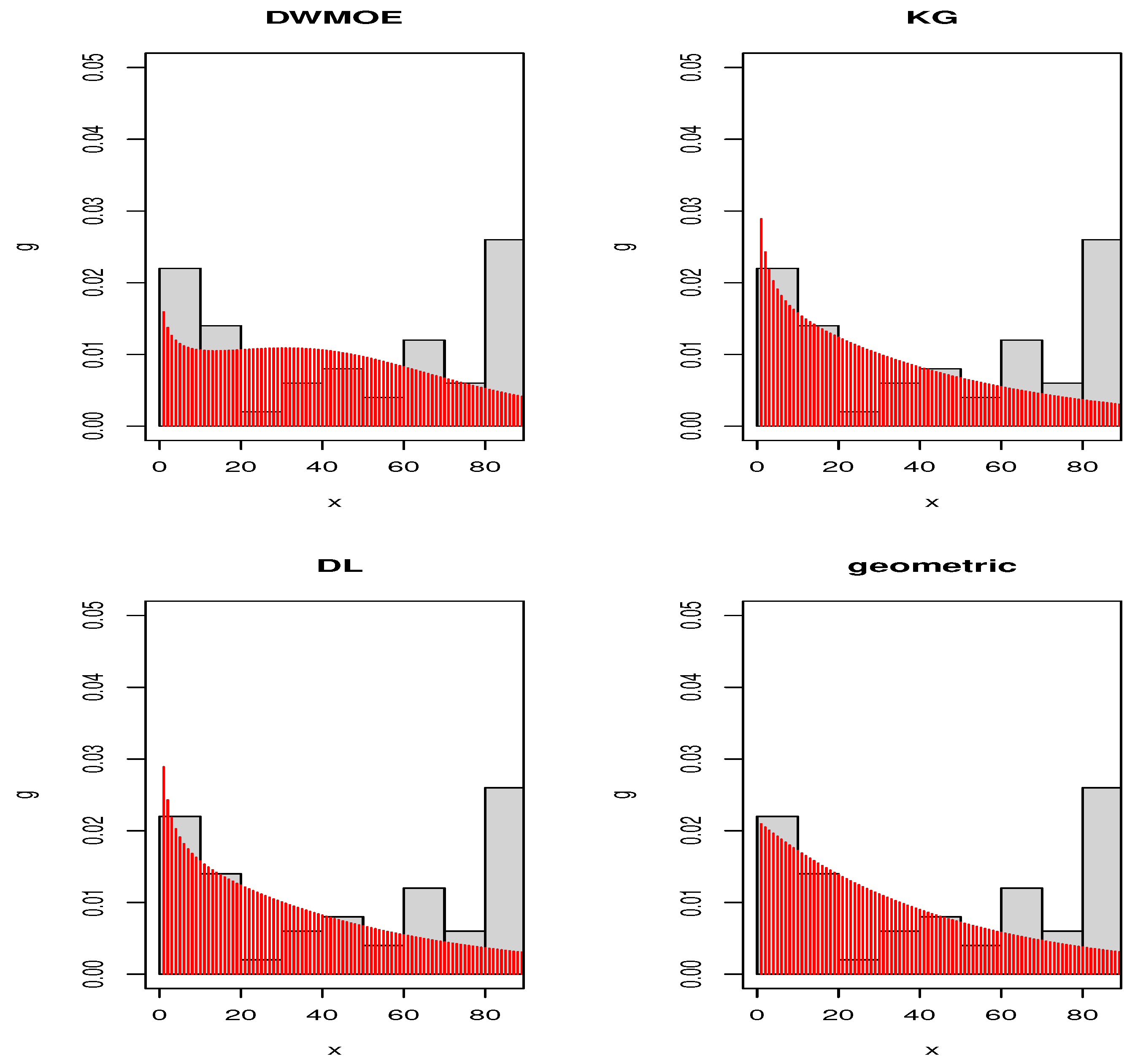
Figure 3 and
Figure 4 give the estimated pdfs for Data set 1 and Data set 2, respectively. These plots also indeed affirm that DWMOE distribution is clearly a competitive model for considered datasets. Thus, the new model may be a best alternative to the considered discrete models for modeling these real data sets.
7. Conclusions
In this paper, we proposed a new discrete Weibull Marshall–Olkin family of distributions with two shape parameters. A special case of this family, discrete Weibull Marshall–Olkin exponential (DWMOE) distribution is studied in detail. The model parameters have been estimated by the maximum likelihood estimation and Bayesian methods. Simulation study is carried out to assess the performance of the different estimation methods. Finally, two real data sets are analyzed to show the importance and flexibility of specified distribution. We hope that the proposed model will serve as a substitute to various discrete distributions exist in Statistical literature.
Author Contributions
Conceptualization, J.G.; Data curation, E.M.A.; Funding acquisition, O.S.B.; Investigation, J.J.; Methodology, J.G.; Project administration, O.S.B.; Resources, J.J.; Software, F.J.; Validation, J.J.; Writing—original draft, J.G.; Writing—review & editing, R.A.K.S. All authors have read and agreed to the published version of the manuscript.
Funding
This manuscript is supported by Digiteknologian TKI-ymparisto project A74338(ERDF, Regional Council of Pohjois-Savo).
Institutional Review Board Statement
Not applicable.
Informed Consent Statement
Not applicable.
Data Availability Statement
Not applicable.
Conflicts of Interest
The authors declare no conflict of interest.
References
- Marshall, A.W.; Olkin, I. A new method for adding a parameter to a family of distributions with application to the exponential and Weibull families. Biometrica 1997, 84, 641–652. [Google Scholar] [CrossRef]
- Castellares, F.; Lemonte, A.J. On the Marshall-Olkin extended distributions. Commun. Stat.-Theory Methods 2016, 45, 4537–4555. [Google Scholar] [CrossRef]
- Cordeiro, G.M.; Lemonte, A.J.; Ortega, E.M.M. The Marshall-Olkin family of distributions: Mathematical properties and new models. J. Stat. Theory Pract. 2014, 8, 343–366. [Google Scholar] [CrossRef]
- Economou, P.; Caroni, C. Parametric proportional odds frailty models. Commun. Stat.-Simul. Comput. 2007, 36, 579–592. [Google Scholar] [CrossRef]
- Lam, K.F.; Leung, T.L. Marginal likelihood estimation for proportional odds models with right censored data. Lifetime Data Anal. 2001, 7, 39–54. [Google Scholar] [CrossRef]
- Nanda, A.K.; Das, S. Stochastic orders of the Marshall-Olkin extended distribution. Stat. Probab. Lett. 2012, 82, 295–302. [Google Scholar] [CrossRef]
- Rao, G.S.; Ghitany, M.E.; Kantam, R.R.L. Reliability test plans for Marshall-Olkin extended exponential distribution. Appl. Math. Sci. 2009, 55, 2745–2755. [Google Scholar]
- Rubio, F.J.; Steel, M.F.J. On the Marshall-Olkin transformation as a skewing mechanism. Comput. Stat. Data Anal. 2012, 56, 2251–2257. [Google Scholar] [CrossRef] [Green Version]
- Tahir, M.H.; Nadarajah, S. Parameter induction in continuous univariate distributions:Well established G families. Ann. Braz. Acad. Sci. 2015, 87, 539–568. [Google Scholar] [CrossRef]
- Jayakumar, K.; Thomas, M. On a generalization of Marshall-Olkin scheme and its application to Burr type XII distribution. Stat. Pap. 2008, 49, 421–439. [Google Scholar] [CrossRef]
- Aly, E.; Benkherouf, E. A new family of distributions based on probability generating functions. Sankhya B-Appl. Interdiscip. Stat. 2011, 73, 70–80. [Google Scholar] [CrossRef]
- Nadarajah, S.; Jayakumar, K.; Ristić, M.M. A new family of lifetime models. J. Stat. Comput. Simul. 2012, 83, 1–16. [Google Scholar] [CrossRef]
- Alizadeh, M.; Cordeiro, G.; Brito, E.; Demétrio, C. The beta Marshall-Olkin family of distributions. J. Stat. Distrib. Appl. 2015, 23, 546–557. [Google Scholar] [CrossRef] [Green Version]
- Alizadeh, M.; Tahir, H.M.; Cordeiro, G.M.; Zubair, M.; Hamedani, G.G. The Kumaraswamy Marshal-Olkin family of distributions. J. Egypt. Math. Soc. 2015, 23, 546–557. [Google Scholar] [CrossRef] [Green Version]
- Sankaran, K.K.; Jayakumar, K. A new extended uniform distribution. International J. Stat. Distrib. Appl. 2016, 2, 35–41. [Google Scholar] [CrossRef] [Green Version]
- Yousof, H.M.; Afify, A.; Nadarajah, S.; Hamedani, G.; Aryal, G. The Marshall-Olkin Generalized-G Family of Distributions with Applications. Statistica 2018, 78, 273–295. [Google Scholar]
- Jayakumar, K.; Sankaran, K.K. Discrete Linnik Weibull distribution. Commun. Stat.-Simul. Comput. 2019, 48, 3092–3117. [Google Scholar] [CrossRef]
- Korkmaz, M.C.; Cordeiro, G.M.; Yousof, H.M.; Pescim, R.R.; Afify, A.Z.; Nadarajah, S. The Weibull Marshall-Olkin family: Regression model and applications to censored data. Commun. Stat.-Theory Methods 2019, 48, 4171–4194. [Google Scholar] [CrossRef]
- Alzaatreh, A.; Lee, C.; Famoye, F. A new method for generating families of continuous distributions. Metron 2013, 71, 63–79. [Google Scholar] [CrossRef] [Green Version]
- Chakraborty, S.; Chakravarty, D. A new discrete probability distribution with integer support on (−∞,∞). Commun. Stat.-Theory Methods 2016, 45, 492–505. [Google Scholar] [CrossRef]
- Krishna, H.; Pundir, P.S. Discrete Burr and discrete Pareto distributions. Stat. Methodol. 2009, 6, 177–188. [Google Scholar] [CrossRef]
- Lisman, J.H.C.; van Zuylen, M.C.A. Note on the generation of the most probable frequency distribution. Stat. Neerl. 1972, 26, 19–23. [Google Scholar] [CrossRef]
- Nakagawa, T.; Osaki, S. The discrete Weibull distribution. IEEE Trans. Reliab. 1975, 24, 300–301. [Google Scholar] [CrossRef]
- Sato, H.; Ikota, M.; Aritoshi, S.; Masuda, H. A new defect distribution meteorology with a consistent discrete exponential formula and its applications. IEEE Trans. Semicond. Manuf. 1999, 12, 409–418. [Google Scholar] [CrossRef]
- Stein, W.E.; Dattero, R. A new discrete Weibull distribution. IEEE Trans. Reliab. 1984, 33, 196–197. [Google Scholar] [CrossRef]
- Jayakumar, K.; Sankaran, K.K. A Discrete Generalization of Marshall-Olkin Scheme and its Application to Geometric Distribution. J. Kerala Stat. Assoc. 2017, 28, 1–21. [Google Scholar]
- Jayakumar, K.; Sankaran, K.K. A generalization of discrete Weibull distribution. Commun. Stat.-Simul. Comput. 2017, 47, 6064–6078. [Google Scholar] [CrossRef]
- Sandhya, E.; Prasanth, C.B. Marshall-Olkin discrete uniform distribution. J. Probab. 2014, 2014, 979312. [Google Scholar] [CrossRef]
- Chakraborty, S. A new discrete distribution related to generalized gamma distribution and its properties. Commun. Stat.-Theory Methods 2015, 44, 1691–1705. [Google Scholar] [CrossRef]
- Cox, D.R.; Hinkley, D.V. Theoretical Statistics; Chapman & Hall: London, UK, 1974. [Google Scholar]
- Bantan, R.; Hassan, A.S.; Almetwally, E.; Elgarhy, M.; Jamal, F.; Chesneau, C.; Elsehetry, M. Bayesian Analysis in Partially Accelerated Life Tests for Weighted Lomax Distribution. CMC-Comput. Mater. Contin. 2021, 68, 2859–2875. [Google Scholar] [CrossRef]
- Sabry, M.A.; Almetwally, E.M.; Alamri, O.A.; Yusuf, M.; Almongy, H.M.; Eldeeb, A.S. Inference of fuzzy reliability model for inverse Rayleigh distribution. Aims Math. 2021, 6, 9770–9785. [Google Scholar] [CrossRef]
- Archer, E.; Park, I.M.; Pillow, J.W. Bayesian entropy estimation for countable discrete distributions. J. Mach. Learn. Res. 2014, 15, 2833–2868. [Google Scholar]
- Ashour, S.K.; Muiftah, M.S.A. Bayesian Estimation of the Parameters of Discrete Weibull Type (I) Distribution. J. Mod. Appl. Stat. Methods 2020, 18, 12. [Google Scholar] [CrossRef]
- Irony, T.Z. Bayesian estimation for discrete distributions. J. Appl. Stat. 1992, 19, 533–549. [Google Scholar] [CrossRef]
- Chen, M.H.; Shao, Q.M. Monte Carlo estimation of Bayesian credible and HPD intervals. J. Comput. Graph. Stat. 1999, 8, 69–92. [Google Scholar]
- Almetwally, E.M.; Ibrahim, G.M. Discrete Alpha Power Inverse Lomax Distribution with Application of COVID-19 Data. Int. J. Appl. Math. Stat. Sci. 2020, 9, 11–22. [Google Scholar]
- Aarset, M.V. How to identify a bathtub hazard rate. IEEE Trans. Reliab. 1987, 36, 106–108. [Google Scholar] [CrossRef]
Figure 1.
pmfs of the DWMOE (, b, ) distribution for some parameter values.
Figure 1.
pmfs of the DWMOE (, b, ) distribution for some parameter values.
Figure 2.
hrfs of the DWMOE(, b, ) distribution for some parameter values.
Figure 2.
hrfs of the DWMOE(, b, ) distribution for some parameter values.
Figure 3.
Plots of estimated pdfs of distributions for Data set 1.
Figure 3.
Plots of estimated pdfs of distributions for Data set 1.
Figure 4.
Plots of estimated pdfs of distributions for Data set 2.
Figure 4.
Plots of estimated pdfs of distributions for Data set 2.
Table 1.
The mean (variance) of DWMOE(, b, ) for different values of parameters.
Table 1.
The mean (variance) of DWMOE(, b, ) for different values of parameters.
| | | 0.2 | 0.5 | 0.7 |
|---|
| | | | | |
| | ↓ | | | |
| | 1.2 | 23.8886 (6880.8534) | 29.2683 (11,009.7047) | 36.9219 (14,310.5902) |
| 0.9 | 23.8283 (6879.0820) | 29.1251 (11,001.4607) | 36.6520 (14,291.7716) |
| | 1.2 | 0.2296 (0.2294) | 1.0254 ( 1.4259) | 2.4205 ( 5.4258) |
| 0.9 | 0.1680 (0.1741) | 0.8224 (1.1803) | 2.0072 (4.5549) |
| | 1.2 | 0.1166 (0.1032) | 0.9268 (0.5908) | 2.2734 (2.0174) |
| 0.9 | 0.0566 (0.0534) | 0.6978 (0.4811) | 1.8268 (1.6304) |
| | 1.2 | 0.0011 (0.0011) | 0.9671 (0.1231) | 2.3879 (0.4845) |
| 0.9 | 8.5316 × (8.5316× ) | 0.7933 (0.1662) | 1.9016 (0.3986) |
| | 1.2 | 1.1009 × ( 1.1009 × ) | 0.9934 (0.0067) | 2.5263 (0.2673) |
| 0.9 | 1.55 × ( 1.55 × ) | 0.9471 (0.0500) | 1.9548 (0.0917) |
Table 2.
Bias, MSE, Lower, and Upper of CIs for parameters of WMOE distribution: Case 1 with different value of .
Table 2.
Bias, MSE, Lower, and Upper of CIs for parameters of WMOE distribution: Case 1 with different value of .
| | | | MLE | Bayesian |
|---|
| n | | Bias | MSE | Lower | Upper | Bias | MSE | Lower | Upper |
| | | | 0.2495 | 0.4825 | 0.9782 | 3.5208 | 0.1108 | 0.1755 | 1.4369 | 2.9437 |
| | 25 | b | 0.3604 | 0.1941 | 0.6137 | 1.6072 | 0.1306 | 0.0272 | 0.6855 | 1.0716 |
| | | | 0.1488 | 0.0276 | 0.2538 | 0.5439 | 0.1339 | 0.0219 | 0.2683 | 0.5074 |
| | | | 0.0522 | 0.1849 | 1.2152 | 2.8893 | 0.0239 | 0.0273 | 1.7041 | 2.3423 |
| 0.25 | 80 | b | 0.2732 | 0.0978 | 0.7251 | 1.3213 | 0.1167 | 0.0215 | 0.6969 | 1.0366 |
| | | | 0.1414 | 0.0241 | 0.2664 | 0.5165 | 0.1206 | 0.0163 | 0.3000 | 0.4651 |
| | | | 0.1958 | 0.1536 | 1.5301 | 2.8615 | 0.0231 | 0.0201 | 1.7841 | 2.3271 |
| | 150 | b | 0.2462 | 0.0711 | 0.7956 | 1.1967 | 0.1311 | 0.0203 | 0.7421 | 1.0302 |
| | | | 0.1380 | 0.0206 | 0.3115 | 0.4645 | 0.1222 | 0.0160 | 0.3077 | 0.4321 |
| | | | −0.0402 | 0.2096 | 1.0459 | 2.8738 | 0.1275 | 0.0408 | 1.9028 | 2.3497 |
| | 25 | b | 0.3161 | 0.1707 | 0.5328 | 1.5994 | 0.1194 | 0.0183 | 0.7461 | 0.9896 |
| | | | 0.0624 | 0.0112 | 0.3906 | 0.7341 | 0.0723 | 0.0060 | 0.4238 | 0.6467 |
| | | | −0.0144 | 0.1235 | 1.1361 | 2.7351 | 0.0249 | 0.0241 | 1.7244 | 2.3009 |
| 0.5 | 80 | b | 0.2003 | 0.0527 | 0.7306 | 1.1700 | 0.0906 | 0.0144 | 0.7017 | 1.0009 |
| | | | 0.0592 | 0.0091 | 0.4885 | 0.6957 | 0.0645 | 0.0058 | 0.5175 | 0.6249 |
| | | | 0.0237 | 0.0337 | 1.6843 | 2.3894 | 0.0240 | 0.0224 | 1.7417 | 2.3112 |
| | 150 | b | 0.1786 | 0.0375 | 0.7814 | 1.0758 | 0.0856 | 0.0135 | 0.6822 | 0.9720 |
| | | | 0.0838 | 0.0079 | 0.5270 | 0.6406 | 0.0230 | 0.0048 | 0.4848 | 0.6360 |
| | | | −0.0706 | 0.1226 | 1.2567 | 2.6021 | 0.0794 | 0.0646 | 1.6848 | 2.5829 |
| | 25 | b | 0.1413 | 0.0406 | 0.6096 | 1.1730 | 0.0397 | 0.0072 | 0.6569 | 0.9542 |
| | | | 0.0102 | 0.0011 | 0.7993 | 0.9211 | −0.0101 | 0.0010 | 0.8169 | 0.8953 |
| | | | −0.0949 | 0.0749 | 1.4013 | 2.4090 | 0.0527 | 0.0627 | 1.5694 | 2.5802 |
| 0.85 | 80 | b | 0.0963 | 0.0146 | 0.7028 | 0.9897 | 0.0547 | 0.0067 | 0.6901 | 0.9238 |
| | | | 0.0142 | 0.0005 | 0.8298 | 0.8987 | 0.0042 | 0.0003 | 0.8225 | 0.8907 |
| | | | −0.0538 | 0.0261 | 1.6475 | 2.2450 | 0.0080 | 0.0238 | 1.7425 | 2.3330 |
| | 150 | b | 0.0871 | 0.0105 | 0.7311 | 0.9431 | 0.0542 | 0.0058 | 0.6958 | 0.9046 |
| | | | 0.0127 | 0.0003 | 0.8411 | 0.8844 | 0.0067 | 0.0002 | 0.8301 | 0.8810 |
Table 3.
Bias, MSE, Lower, and Upper of CIs for parameters of WMOE distribution: Case 2 with different value of .
Table 3.
Bias, MSE, Lower, and Upper of CIs for parameters of WMOE distribution: Case 2 with different value of .
| | | | MLE | Bayesian |
|---|
| n | | Bias | MSE | Lower | Upper | Bias | MSE | Lower | Upper |
| | | | 0.3139 | 0.1366 | 1.9312 | 2.6966 | 0.1365 | 0.0751 | 1.6867 | 2.5906 |
| | 25 | b | 0.9532 | 1.2137 | 1.8699 | 4.0364 | 0.1257 | 0.0248 | 1.9302 | 2.3134 |
| | | | 0.1161 | 0.0145 | 0.3031 | 0.4292 | 0.1026 | 0.0141 | 0.2932 | 0.4037 |
| | | | 0.2935 | 0.0954 | 2.1048 | 2.4821 | 0.0493 | 0.0250 | 1.7261 | 2.3206 |
| 0.25 | 80 | b | 0.9093 | 0.9120 | 2.3368 | 3.4818 | 0.0948 | 0.0209 | 1.8694 | 2.2937 |
| | | | 0.1204 | 0.0141 | 0.3432 | 0.3976 | 0.1123 | 0.0138 | 0.3418 | 0.4161 |
| | | | 0.2742 | 0.0787 | 2.1572 | 2.3912 | 0.0505 | 0.0175 | 1.7838 | 2.2669 |
| | 150 | b | 0.9100 | 0.8728 | 2.4952 | 3.3248 | 0.0762 | 0.0088 | 1.9658 | 2.1777 |
| | | | 0.1122 | 0.0135 | 0.3051 | 0.3993 | 0.1027 | 0.0124 | 0.3483 | 0.4075 |
| | | | 0.1388 | 0.0416 | 1.8460 | 2.4317 | 0.1110 | 0.0407 | 1.8659 | 2.4055 |
| | 25 | b | 0.5284 | 0.4035 | 1.8371 | 3.2198 | 0.0590 | 0.0070 | 1.9559 | 2.1861 |
| | | | 0.0600 | 0.0042 | 0.5116 | 0.6084 | 0.0591 | 0.0040 | 0.5232 | 0.6014 |
| | | | 0.1404 | 0.0261 | 1.9833 | 2.2974 | 0.0362 | 0.0241 | 1.7758 | 2.3729 |
| 0.5 | 80 | b | 0.5210 | 0.3119 | 2.1266 | 2.9154 | 0.0670 | 0.0060 | 2.1868 | 2.2654 |
| | | | 0.0627 | 0.0041 | 0.5358 | 0.5896 | 0.0624 | 0.0040 | 0.5327 | 0.5860 |
| | | | 0.1070 | 0.0124 | 1.7852 | 2.2510 | 0.0246 | 0.0121 | 2.0471 | 2.1669 |
| | 150 | b | 0.3693 | 0.1465 | 1.9060 | 2.2538 | 0.0589 | 0.0058 | 2.1972 | 2.2566 |
| | | | 0.0626 | 0.0040 | 0.5367 | 0.5915 | 0.0630 | 0.0039 | 0.5440 | 0.5812 |
| | | | 0.0117 | 0.0028 | 1.9101 | 2.1133 | 0.0095 | 0.0021 | 1.9548 | 2.1258 |
| | 25 | b | 0.0584 | 0.0217 | 1.7930 | 2.3238 | 0.0159 | 0.0055 | 1.8639 | 2.1513 |
| | | | 0.0048 | 0.00013 | 0.8341 | 0.8755 | 0.0043 | 0.00012 | 0.8279 | 0.8804 |
| | | | 0.0242 | 0.0023 | 1.9423 | 2.1061 | 0.0038 | 0.0020 | 1.9735 | 2.2802 |
| 0.85 | 80 | b | 0.0563 | 0.0208 | 1.8565 | 2.3562 | 0.0225 | 0.0019 | 1.8279 | 2.2248 |
| | | | 0.0061 | 0.00008 | 0.8439 | 0.8683 | 0.0060 | 0.00007 | 0.8421 | 0.8707 |
| | | | 0.0082 | 0.00015 | 1.9908 | 2.0256 | 0.0036 | 0.00010 | 1.9978 | 2.0210 |
| | 150 | b | 0.0324 | 0.0020 | 1.9708 | 2.0940 | 0.0211 | 0.0018 | 1.9855 | 2.0919 |
| | | | 0.0062 | 0.00006 | 0.8482 | 0.8642 | 0.0061 | 0.00005 | 0.8456 | 0.8675 |
Table 4.
Bias, MSE, Lower, and Upper of CIs for parameters of WMOE distribution: Case 3 with different value of .
Table 4.
Bias, MSE, Lower, and Upper of CIs for parameters of WMOE distribution: Case 3 with different value of .
| | | | MLE | Bayesian |
|---|
| n | | Bias | MSE | Lower | Upper | Bias | MSE | Lower | Upper |
| | | | 0.6215 | 0.4291 | 0.8654 | 1.6776 | 0.2448 | 0.1164 | 0.5450 | 1.3491 |
| | 25 | b | 0.8058 | 0.7366 | 2.2257 | 3.3858 | 0.0258 | 0.0304 | 1.9406 | 2.1294 |
| | | | 0.1794 | 0.0761 | 0.2583 | 0.4004 | 0.1764 | 0.0534 | 0.3045 | 0.5271 |
| | | | 0.3994 | 0.1825 | 0.7521 | 1.3466 | 0.0977 | 0.0284 | 0.5057 | 1.0224 |
| 0.25 | 80 | b | 0.4832 | 0.2835 | 2.0445 | 2.9219 | 0.0287 | 0.0138 | 1.8191 | 2.2592 |
| | | | 0.1236 | 0.0157 | 0.3341 | 0.4132 | 0.1087 | 0.0137 | 0.3512 | 0.5246 |
| | | | 0.2488 | 0.1497 | 0.6930 | 1.3647 | 0.1178 | 0.0231 | 0.5419 | 0.9682 |
| | 150 | b | 0.3610 | 0.1964 | 2.3010 | 2.9082 | 0.0428 | 0.0118 | 1.8586 | 2.2454 |
| | | | 0.1068 | 0.0118 | 0.3159 | 0.3976 | 0.0836 | 0.0104 | 0.3642 | 0.5011 |
| | | | 0.5223 | 0.3338 | 0.6880 | 1.6566 | 0.3891 | 0.2432 | 0.5403 | 1.5798 |
| | 25 | b | 0.7786 | 0.7465 | 2.0440 | 3.5131 | 0.0641 | 0.0702 | 1.9507 | 2.1617 |
| | | | 0.0122 | 0.0030 | 0.4072 | 0.6172 | 0.0453 | 0.0030 | 0.4242 | 0.6474 |
| | | | 0.3975 | 0.1886 | 0.7011 | 1.3939 | 0.1113 | 0.0291 | 0.4944 | 0.9766 |
| 0.5 | 80 | b | 0.6600 | 0.4671 | 2.3084 | 3.0117 | 0.0572 | 0.0147 | 1.8994 | 2.2347 |
| | | | 0.0382 | 0.0029 | 0.4634 | 0.6129 | 0.0359 | 0.0028 | 0.5204 | 0.6423 |
| | | | 0.3428 | 0.1849 | 0.8647 | 1.2903 | 0.1206 | 0.0261 | 0.5750 | 0.9880 |
| | 150 | b | 0.6597 | 0.4553 | 2.3812 | 2.9382 | 0.0490 | 0.0121 | 1.9415 | 2.3053 |
| | | | 0.0289 | 0.0014 | 0.4814 | 0.5764 | 0.0218 | 0.0013 | 0.5306 | 0.6450 |
| | | | 0.1351 | 0.0477 | 0.4457 | 1.1245 | 0.1219 | 0.0411 | 0.5329 | 1.3685 |
| | 25 | b | 0.2723 | 0.1236 | 1.8326 | 2.7121 | 0.0746 | 0.0151 | 1.9471 | 2.3112 |
| | | | 0.0021 | 0.0004 | 0.8105 | 0.8938 | −0.0046 | 0.0004 | 0.8183 | 0.8853 |
| | | | 0.1386 | 0.0343 | 0.5382 | 1.0390 | 0.0405 | 0.0122 | 0.4971 | 0.9237 |
| 0.85 | 80 | b | 0.2066 | 0.0756 | 1.8366 | 2.5767 | 0.0504 | 0.0103 | 1.8674 | 2.2138 |
| | | | −0.0017 | 0.0002 | 0.8191 | 0.8776 | 0.0016 | 0.0002 | 0.8215 | 0.8798 |
| | | | 0.1274 | 0.0212 | 0.6385 | 0.9163 | 0.0591 | 0.0120 | 0.5335 | 0.8672 |
| | 150 | b | 0.1926 | 0.0727 | 2.0980 | 2.4304 | 0.0208 | 0.0056 | 1.9020 | 2.1739 |
| | | | 0.0065 | 0.0002 | 0.7832 | 0.8299 | 0.0041 | 0.0002 | 0.7858 | 0.8482 |
Table 5.
Estimated values, −logL, AIC, BIC, K-S statistics, p-value, and for data set 1.
Table 5.
Estimated values, −logL, AIC, BIC, K-S statistics, p-value, and for data set 1.
| Distribution | Estimates(SE) | −logL | AIC | BIC | K-S | p-Value | | |
|---|
| DWMOE | = 1657.1914 | 91.11431 | 188.2286 | 192.6258 | 0.1209 | 0.737 | 0.54066 | 0.0831 |
| | (4233.4787) | | | | | | | |
| | = 0.421(0.1050) | | | | | | | |
| | = 0.3446 (0.5445) | | | | | | | |
| KG | = 3.1744(0.0171) | 94.9914 | 195.9828 | 200.38 | 0.19379 | 0.1807 | 1.89 | 0.2395 |
| | = 0.2943(0.0526) | | | | | | | |
| | = 0.5717(0.0062) | | | | | | | |
| DL | = 3.1744(0.0171) | 97.12205 | 196.2441 | 197.7098 | 0.1620 | 0.3703 | 1.3817 | 0.1894 |
| geometric | = 0.1194 (0.0198) | 98.01666 | 198.0333 | 199.499 | 0.25464 | 0.03153 | 1.3817 | 0.1894 |
Table 6.
Estimated values, −logL, AIC, BIC, K-S statistics, p-value, and for data set 2.
Table 6.
Estimated values, −logL, AIC, BIC, K-S statistics, p-value, and for data set 2.
| Distribution | Estimates(SE) | −logL | AIC | BIC | K-S | p-Value | | |
|---|
| DWMOE | = 11.5621(12.5867) | 238.0759 | 482.1519 | 487.8879 | 0.17892 | 0.0814 | 2.364 | 0.3069 |
| | = 0.6771(0.1510) | | | | | | | |
| | = 0.9488(0.0138) | | | | | | | |
| KG | =0.4987(0.3082) | 240.1928 | 486.3855 | 492.1216 | 0.1855 | 0.0641 | 2.876 | 0.4761 |
| | = 0.1129(0.1299) | | | | | | | |
| | = 0.8367(0.1758) | | | | | | | |
| DL | = 0.0424(0.0042) | 249.9767 | 501.9534 | 503.8654 | 0.20147 | 0.0345 | 6.2977 | 0.6529 |
| geometric | = 0.02142(0.0030) | 241.6264 | 485.2527 | 487.1647 | 0.19310 | 0.048 | 0.1931 | 3.0769 |
| Publisher’s Note: MDPI stays neutral with regard to jurisdictional claims in published maps and institutional affiliations. |
© 2021 by the authors. Licensee MDPI, Basel, Switzerland. This article is an open access article distributed under the terms and conditions of the Creative Commons Attribution (CC BY) license (https://creativecommons.org/licenses/by/4.0/).


 ,
, 


