Article

Ranking Road Sections Based on MCDM Model: New Improved Fuzzy SWARA (IMF SWARA)

1
College of Engineering and Technology, American University of the Middle East, Street 250, Block 6, Egaila 54200, Kuwait
2
Technical Faculty, University of Bihac, Irfana Ljubijankića bb, 77000 Bihać, Bosnia and Herzegovina
3
Faculty of Transport and Traffic Engineering, University of East Sarajevo, Vojvode Mišića 52, 74000 Doboj, Bosnia and Herzegovina
4
Faculty of Engineering and Natural Sciences, International Burch University, Francuske revolucije bb, Ilidža, 71210 Sarajevo, Bosnia and Herzegovina
*
Author to whom correspondence should be addressed.
Axioms 2021, 10(2), 92; https://doi.org/10.3390/axioms10020092
Submission received: 21 April 2021 / Revised: 11 May 2021 / Accepted: 13 May 2021 / Published: 15 May 2021
(This article belongs to the Special Issue Modern Problems of Mathematical Physics and Their Applications)

Abstract

:
Traffic management is a significantly difficult and demanding task. It is necessary to know the main parameters of road networks in order to adequately meet traffic management requirements. Through this paper, an integrated fuzzy model for ranking road sections based on four inputs and four outputs was developed. The goal was to determine the safety degree of the observed road sections by the methodology developed. The greatest contribution of the paper is reflected in the development of the improved fuzzy step-wise weight assessment ratio analysis (IMF SWARA) method and integration with the fuzzy measurement alternatives and ranking according to the compromise solution (fuzzy MARCOS) method. First, the data envelopment analysis (DEA) model was applied, showing that three road sections have a high traffic risk. After that, IMF SWARA was applied to determine the values of the weight coefficients of the criteria, and the fuzzy MARCOS method was used for the final ranking of the sections. The obtained results were verified through a three-phase sensitivity analysis with an emphasis on forming 40 new scenarios in which input values were simulated. The stability of the model was proven in all phases of sensitivity analysis.
MSC:
90B20; 90B50; 90C08

1. Introduction

Roads represent considerable resources and are some of the most important public investments of a country, with significant funds allocated for their construction and maintenance with two main tasks: that they are efficient and safe. In a real traffic flow, almost all functional dependencies given by international road standards are based on the correlation between flow, speed, density, number of traffic accidents, etc., as traffic parameters and longitudinal gradient, minimum radius of horizontal curve, etc., as road parameters. The analysis of functional dependence requires special attention and is particularly evident for two-lane roads, since these roads make up the largest percentage of a road network of a country. Based on the research [1] conducted on 3450 km stretch of two-lane roads in Valencia, it was shown that traffic risk is significantly affected by the density of access points, average sight distance, average speed limit, and the proportion of no-passing zones. The impact of a larger number of access points also results in a large number of conflict points on the road, which significantly affects both speed and flow, as well as a negative trend in safety for traffic participants.
Deviation from speed limits is most often associated with an increased probability of traffic accidents. In addition, any credible deviation from the speed limit of real traffic flow is an imperative in the analysis of speeding, and thus the potential occurrence of incidents. Speed credibility analysis is a method of traffic engineering management which is often neglected and can lead to worsening traffic risk. Any deviation from speed limits is often related to both technical and operational road characteristics, as well as to the psychophysical abilities of drivers. For example, across slope ranges of −5.5% to 4.50%, it was found that speed increases with where the slope increases, and with a decrease, stress while driving increases too [2]. Within this research, measured sections on the slope were identified as potential places with a high percentage of traffic accidents. According to the research [3], about 40% of drivers drove above the permitted speed limit, and this percentage of speeding varies from location to location. It was concluded that the speed limit of 60 km/h was not appropriate for most of the investigated locations.
In traffic and operational analyzes conducted on two-lane roads, unadjusted speed is one of key indicators for the occurrence of traffic accidents. The importance of the 85th percentile speed is especially emphasized in the scientific literature, since it is a representative speed in a traffic flow of road network users [3,4]. Commonly, the number of traffic accidents and an increase in risk are related to the exploitation speed. Exploitation speeds have been shown to be higher than design speeds for a speed limit of about 55 mph or less. Therefore, it is important to present speed potentially through five specific indicators of speed dependence on geometric road characteristics [5].
In addition to the importance of the research field and motivation for conducting this study, it is very important to emphasize that in addition to the professional contribution reflected in assessing the safety level of considered sections, a significant scientific contribution was made too. It is reflected through forming an integrated fuzzy multi-criteria decision-making (MCDM) model with an emphasis on defining the IMF SWARA method that eliminates the shortcomings of the previously developed fuzzy SWARA method, which is explained in detail in the Materials and Methods section. It is also important to emphasize that Dombi and Bonferroni aggregators were used to average specific values of inputs and outputs.
After the introduction in Section 1, the rest of the paper is structured as follows. Section 2 provides an overview of the literature related to the field of application. Section 3 presents the preliminaries regarding the development of the methodology. Section 4 presents the creation of the methodology that is described and explained in detail. Section 5 provides a case study with a detailed calculation given for each approach of the methodology proposed. Section 6 demonstrates the stability of the model through a three-phase sensitivity analysis, while Section 7 presents a conclusion with guidelines for further research.

2. Literature Review

Contemporary HCM methodology [6], depending on the speed limit, can classify all two-lane roads in Bosnia and Herzegovina in class II of two-lane roads (where limit speed does not exceed 80 km/h), and the assessment of the qualitative measure level of service (LOS) is based on determining the percentage of time losses, but not on the mean value of speed or deviation from the speed limit. The German methodology HBS 2001 [7] mainly expresses the problem of the functional dependence of travel speed on the width of traffic lanes. This method defines a minimum lane width of 2.75 m, while the lane width can be 2.50 m on some sections of road in Bosnia and Herzegovina. Chapter 10 of the Highway Safety Manual [8] (HSM, 2010) defines a method for predicting traffic accidents for suburban two-lane, two-way roads. This prediction method provides a procedure consisting of 18 steps for estimating the “expected average number of traffic accidents” (according to the total number of accidents, the severity of accidents, or the type of collision) on road networks, facilities, or locations.
However, some authors have investigated the functional dependence of speed, length of individual geometric road elements, radius of curvature of transverse/longitudinal slopes, and traffic accidents [9,10,11,12]. Additionally, in some research the problem of reducing speed due to geometric road characteristics arises. The reduction in speed of heavy vehicles was specifically analyzed in a study where a longitudinal slope of 9.0% at 1.20 km of road was included, showing a significant reduction in the speed of heavy vehicles. According to this study, in order to increase speed due to influential road factors, power-to-mass ratio must be improved [13]. Based on a report conducted in Texas [14], regression analysis determined that the following variables affect the prediction of traffic accidents: AADT, lane width, shoulder width, and section length. The use of wider longitudinal road markings leads to a reduction in the speed of vehicles, and thus a reduction in the number of traffic accidents. The analysis of speed reduction in day and night driving conditions at average traffic volume showed the following reduction in vehicle speed: 2.24% during the day and 1.96% at night for light vehicles, and 2.46% during the day and 2.15% at night for heavy vehicles [15]. Using the Bayesian network analysis for predicting the probability of the influence of traffic and road factors on the occurrence of traffic accidents, it is especially emphasized that vehicle speed, horizontal curve radius, vehicle type, adhesion coefficient, and longitudinal slope are important factors [11]. Additionally, the results of the study [12] show that the continuous use of several boundary indices and the excessive average gradient of long and steep road sections are some of the main causes of frequent accidents on the Hexi section.
In a study conducted according to data on 465 traffic accidents in Chongqing, vehicle stability is analyzed as a function of a combination of steep slopes and the sharp radii of curves, where a relevant safety model of a combined section of a steep slope and sharp curve was established. The simulation iteration frequency at 100 Hz (using the target speed control mode) was performed on steep downhills where safety factors were analyzed downhill at speeds of 40 km/h, 60 km/h, and 80 km/h [16]. Additionally, in a study researching the validation of mean speeds collected in a driving simulator, speed was monitored on curves corresponding to real-world road sections. A road in Iran was simulated in two experiments. In the first experiment, the speeds of 30 participants were collected at the beginning, middle, and end of five curves, and in the second experiment, the speeds of 40 different participants were collected at specified points of five curves on the real road using radar. In most curves, the mean speeds in the simulator were higher than on the real road, and the trend in changing speed from the beginning to the end of the curve was similar in both experiments [17]. Additionally, the dynamic simulation procedure analyzed several factors (longitudinal grades, minimum radius of horizontal curve, vehicle speed, changes in vehicle length and weight, and differences in changes in driver behavior) where the level of traffic safety was determined across large radius curves. This research demonstrates the need for the introduction of clothoid transition curves, and also proposed a methodology for the analysis of lateral friction for speeds of 50, 80, 110, and 130 km/h [18]. At the same time, the analysis of lateral friction, through the reduction of the coefficient of friction by 5% in vertical curves, increased the probability of a traffic accident by 20% for rescue vehicles. By increasing the speed of these vehicles in curves by 10%, the probability of a crash increases by 25% [19]. Some researchers have analyzed roads in rural areas in order to determine the functional correlation between vehicle speed at different horizontal radii of curves in order to link this to traffic safety. Within this research, a linear model for predicting operating speeds depending on the radius and preceding tangent length of the curve was developed [20].
The implementation of different approaches in one integrated model is a practice that very often ensures more accurate results. Such models are preferable, thus many researchers have brought new ideas and have implemented them in the field of transport and traffic. For example, an approach based on an individual DEA for determining the efficiency of 197 municipalities containing two inputs and 14 outputs was applied in [21]. The obtained results showed that due to the weights of the input, it was possible for a more efficient municipality to be ranked lower. In the study [22] the analytic hierarchy process (AHP) method for determining the influence of traffic factor interaction on the rate of traffic accidents was applied. The MCDM model was also applied in [23] for the identification of priority black spots in order to decrease traffic risk, while in [24] authors have implemented the AHP method in order to evaluate and rank road section designs. In the research [25], a new multi-criteria and simultaneous multi-objective optimization (MOO) model using the AHP method for evaluating and ranking traffic and geometric elements was created.
For transport projects, policies, or policy measures, various multi-criteria methods have been used. The study [26] defines why MCDM models play such an important role in dealing with various categories of decision problems that arise in mass transit systems. Additionally, the importance of MCDM models in this field has been proven with two case studies. In the study [27], a novel hybrid model which combines the fuzzy step-wise weight assessment ratio analysis (FSWARA) and the fuzzy best-worst method (FBWM) was developed for selection of equipment in a container terminal. By applying MCDM, the quality of life in urban environments was assessed at three spatial levels (socioeconomic, environmental, and accessibility) [28]. For transport projects, policies, or the evaluation of policy measures, from 1982 to 2019 we have seen the development and effective application of various multi-criteria methods to complement conventional cost effectiveness and cost benefit analyses [29]. The determination of transportation and traffic risk is a very popular and interesting activity that can help participants avoid risk and conflict situations. The authors in [30] applied a fuzzy pivot pairwise relative criteria importance assessment (Fuzzy PIPRECIA) method to determine and rank the road transportation risk factors in the Giresun province.

3. Preliminaries

3.1. Preliminaries—Operations with Fuzzy Numbers

A fuzzy number A ¯ on R is to be a TFN if its membership function μ A ¯ ( x ) : R→[0,1] is equal to following Equation (1) [31,32]:
μ A ¯ ( x ) = { x l m l l x m u x u m m x u 0 o t h e r w i s e
In Equation (1), l and u indicated the lower and upper bounds of the fuzzy number A ¯ , and m is the modal value for A ¯ . The TFN can be denoted by A ¯ = ( l , m , u ) .
The operational laws of TFN A ¯ = ( l 1 , m 1 , u 1 ) and A ¯ = ( l 2 , m 2 , u 2 ) are displayed as the following equations.
Addition:
A 1 ¯ + A 2 ¯ = ( l 1 , m 1 , u 1 ) + ( l 2 , m 2 , u 2 ) = ( l 1 + l 2 , m 1 + m 2 , u 1 + u 2 )
Multiplication:
A 1 ¯ × A 2 ¯ = ( l 1 , m 1 , u 1 ) × ( l 2 , m 2 , u 2 ) = ( l 1 × l 2 , m 1 × m 2 , u 1 × u 2 )
Subtraction:
A 1 ¯ A 2 ¯ = ( l 1 , m 1 , u 1 ) ( l 2 , m 2 , u 2 ) = ( l 1 u 2 , m 1 m 2 , u 1 l 2 )
Division:
A 1 ¯ A 2 ¯ = ( l 1 , m 1 , u 1 ) ( l 2 , m 2 , u 2 ) = ( l 1 u 2 , m 1 m 2 , u 1 l 2 )
Reciprocal:
A 1 ¯ 1 = ( l 1 , m 1 , u 1 ) 1 = ( 1 u 1 , 1 m 1 , 1 l 1 )

3.2. Preliminaries—Dombi Aggregator

The Dombi aggregator [33] was used to determine the value of AADT, since data for a total of 12 years were considered.
( b j ) = j = 1 n ( b j ) 1 + ( j = 1 n w j ( 1 f ( b j ) f ( b j ) ) ) f ( b j ) = b j j = 1 n b j
where wj represents the weight of each considered year of data separately.

3.3. Preliminaries—Bonferroni Aggregator

Since the previous Dombi aggregator is not suitable for averaging the value of traffic accidents due to the occurrence of the value of zero, the Bonferroni aggregator was used [34].
a j = ( 1 e ( e 1 ) i , j = 1 i j e a i p a j q ) 1 p + q
In this research, e represents the number of years for traffic accidents, while p, q ≥ 0 are a set of non-negative numbers.

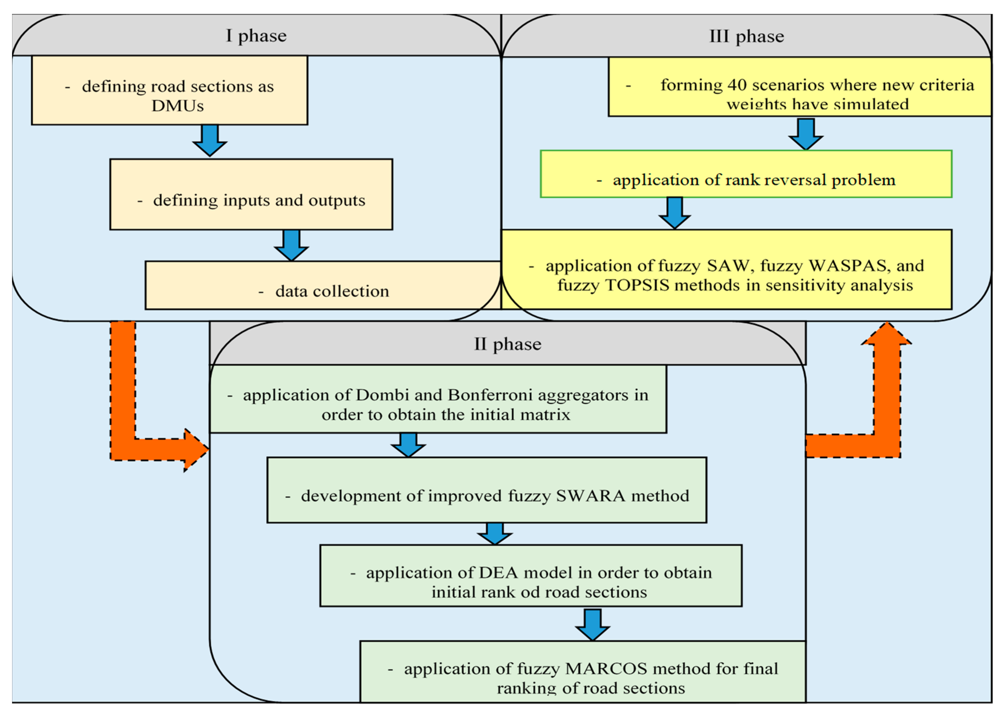
4. Materials and Methods

This section presents the main phases of the research with the methodology created for determining the safety degree of road sections. All phases and the overall methodology are described below and shown in Figure 1, consisting of a total of 10 steps arranged in three phases which are causally connected.

4.1. The First Phase

The first phase is to define sections of road infrastructure, determine entrances and exits, and collect data. A total of six sections of the road network on the territory of the Republic of Srpska were considered: Vrhovi-Šešlije I, Vrhovi-Šešlije II, Rudanka-Doboj, Šepak-Karakaj 3, Donje Caparde-Karakaj 1, and Border (RS/FBIH)-Donje Caparde. The input parameters for the given sections were as follows: section length—I1, road slope—I2, deviation from the speed limit—I3, and average annual daily traffic (AADT) —I4. The classifications of traffic accidents with fatalities, severe injuries, minor injuries, and material damage are defined as output parameters, O1, O2, O3, and O4, respectively.

4.2. The Second Phase

The second phase is the most important part of this research as it develops a methodology for determining the safety degree of certain road sections. After collecting all data from the first phase, it is necessary to determine an initial matrix that synthesizes the input and output parameters of the model. In terms of input data, AADT in the last 12 years has been considered as a very important factor in both this analysis and others. Since the data refer to a large number of years in order to obtain unique values, the Dombi aggregator described in the previous section was applied. The traffic parameters that occurred in the last five years on the presented road sections were considered as output parameters. Since no traffic accidents with fatalities occurred on certain sections during the year, i.e., their value was zero, the Bonferroni aggregator, also described in the previous section, was used.

4.2.1. Improved Fuzzy SWARA Method (IMF SWARA)

Step 1: After defining all the criteria on the basis of which the decision was made, it is necessary to arrange them in descending order based on their expected significance. For example, the most significant criterion is placed in first position and the least significant criterion is in the last position.
Step 2: Starting from the previously determined rank, the relatively smaller significance of the criterion (criterion Cj) was determined in relation to the previous one (Cj−1), and this was repeated for each subsequent criterion. This relation, i.e., comparative significance of the average value, is denoted with s j ¯ . A key problem in the original fuzzy SWARA [35] method is the application of an inadequate scale to determine the comparative significance of criteria, as demonstrated in detail below. Therefore, in this paper, the key point that improves the fuzzy SWARA method is the development of an adequate TFN scale (Table 1) that enables the precise and good quality determination of the significance of criteria using improved fuzzy SWARA (IMF SWARA).
Step 3: Determining the fuzzy coefficient k j ¯ (9):
k j ¯ = { 1 ¯ j = 1 s j ¯ j > 1
Step 4: Determining the calculated weights q j ¯ (10):
q j ¯ = { 1 ¯ j = 1 q j 1 ¯ k j ¯ j > 1
Step 5: Calculation of the fuzzy weight coefficients using the following Equation (11):
w j ¯ = q j ¯ j = 1 m q j ¯
where wj represents the fuzzy relative weight of the criteria j, and m represents the total number of criteria.
We will now present the reasoning behind the need to develop the improved fuzzy SWARA (IMF SWARA) method, i.e., why the original fuzzy SWARA method [35] was not well conceived. To do this we have taken two examples, both from the paper in which the original extension of the fuzzy SWARA method was performed. The authors considered four main criteria: economic, environmental, social, and risk, applying the scale developed by Chang in 1996 [36] for the purposes of calculating the weights of criteria using the fuzzy AHP method, as shown in Table 2.
Therefore, the authors in developing the fuzzy SWARA method in [35] should not have used the scale created for the fuzzy AHP method, since the procedure for solving and thus evaluating the criteria is different for these two methods. The authors obtained the values of the criteria as shown in Table 3. As can be seen, the evaluation was performed as follows: less important, much less important, and moderately less important, respectively.
The calculation below instead applies the improved fuzzy SWARA (IMF SWARA) (Table 4) method developed in this paper using the same linguistic variables: LS, MLS, and MDLS in order to show differences in the obtained fuzzy weights.
Considering the comparative analysis on the basis of the same example by applying both the fuzzy SWARA and improved fuzzy SWARA (IMF SWARA) method, three key points can be identified:
(1) Using the fuzzy SWARA method, it is impossible to obtain results in which two criteria have equal fuzzy weights. By applying the improved fuzzy SWARA method, two or more criteria can have equal values.
(2) On the contrary, applying the inadequate TFN scale shown in Table 2, where decision-makers indicate that two criteria have the same value by assigning TFN (1,1,1), the criterion Cj in relation to Cj−1 received a value that is twice less than Cj. By applying the improved fuzzy SWARA method, assigning the value (0,0,0), equal values are obtained and not values twice as large.
(3) By increasing the number of criteria in the model, the least significant criteria receive values that can be negligible, i.e., with a tendency to zero. By applying the improved fuzzy SWARA method, less significant criteria have higher values and can play a greater role in the decision-making process.
We prove the above through a comparative analysis of the second example, which is a continuation of the first one. Namely, it is further considered the sub-criteria of the main economic criterion, which contains a total of eight criteria. A comparative analysis from which the inadequacy of the results of the fuzzy SWARA method can be concluded and the advantages of the improved fuzzy SWARA (IMF SWARA) method are shown in Table 5.
In Table 5, we prove that all three key points were enhanced through the development of the improved fuzzy SWARA (IMF SWARA) method. As can be observed using the fuzzy SWARA method, there is no case where two criteria have the same weight, although in the process of the criterion evaluation it is indicated that criteria C5 and C6 should have equal values. If, using the fuzzy SWARA method, we see that criterion C6 is assigned TFN (1,1,1), this should mean that it has the same value as the preceding C5 criterion. However, the results show that C5 is twice as important as C6, which is an inconsistency in the process of evaluating the criteria and its weights. This shortcoming is eliminated by applying the improved fuzzy SWARA (IMF SWARA) method, which can be seen in Table 5. Additionally, it is evident that less significant criteria with an increase in the total number of criteria do not have a maximum tendency to zero.
Some examples of the application of the fuzzy SWARA method with an inadequate scale were given in studies [37,38,39,40]. It should be noted that the future application of the fuzzy SWARA method should be replaced by the improved fuzzy SWARA (IMF SWARA) method or the application of another scale in fuzzy SWARA that eliminates these previously observed shortcomings.

4.2.2. DEA Model

The CCR model is the most basic model of DEA [41,42]. Here, two DEA CCR models have been formed according to an input-oriented model (max) and according to an output-oriented model (min). The DEA CCR input-oriented model (max) is:
D E A i n p u t = max i = 1 m w i x i i n p u t s t : i = 1 m w i x i j i = m + 1 m + s w i y i j 0 , j = 1 , , n i = m + 1 m + s w i y i o u t p u t = 1 w i 0 , i = 1 , , m + s
The decision-making units (DMUs) are presented as m inputs for each alternative xij, through s which represents outputs for each alternative yij. Additionally, the weights of the parameters wi are taken into account [43]. The total number of DMUs is denoted by n.
The DEA CCR output-oriented model (min) is:
D E A o u t p u t = min i = m + 1 m + s w i y i o u t p u t s t : ( i = 1 m w i x i j ) + i = m + 1 m + s w i y i j 0 , j = 1 , , n i = 1 m w i x i i n p u t = 1 w i 0 , i = 1 , , m + s

4.2.3. Fuzzy MARCOS Method

The fuzzy MARCOS method was developed by Stanković et al. [44] and consists of the following steps [45]:
Step 1. Forming an initial fuzzy decision matrix.
Step 2. Expanding the initial fuzzy decision matrix with an anti-ideal solution (AAI):
A ˜ ( A I ) = min i x ˜ i j i f j B a n d max i x ˜ i j i f j C
and the ideal solution (AI):
A ˜ ( I D ) = max i x ˜ i j i f j B a n d min i x ˜ i j i f j C
Step 3. Normalizing the initial fuzzy decision matrix.
n ˜ i j = ( n i j l , n i j m , n i j u ) = ( x i d l x i j u , x i d l x i j m , x i d l x i j l ) i f j C
n ˜ i j = ( n i j l , n i j m , n i j u ) = ( x i j l x i d u , x i j m x i d u , x i j u x i d u ) i f j B
Step 4. Weighting the normalized decision matrix.
v ˜ i j = ( v i j l , v i j m , v i j u ) = n ˜ i j w ˜ j = ( n i j l × w j l , n i j m × w j m , n i j u × w j u )
Step 5. Calculating the Si matrix:
S ˜ i = i = 1 n v ˜ i j
Step 6. Calculating the degree of usefulness Ki.
K ˜ i = S ˜ i S ˜ a i = ( s i l s a i u , s i m s a i m , s i u s a i l )
K ˜ i + = S ˜ i S ˜ i d = ( s i l s i d u , s i m s i d m , s i u s i d l )
Step 7. Calculating the fuzzy matrix T ˜ i .
T ˜ i = t ˜ i = ( t i l , t i m , t i u ) = K ˜ i K ˜ i + = ( k i l + k i + l , k i m + k i + m , k i u + k i + u )
Determining the fuzzy number D ˜ :
D ˜ = ( d l , d m , d u ) = max i t ˜ i j
Step 8. The de-fuzzification of fuzzy numbers:
d f c r i s p = l + 4 m + u 6
Step 9. Determining the utility function f ( K ˜ i ) :
Utility function according to the anti-ideal solution.
f ( K ˜ i + ) = K ˜ i d f c r i s p = ( k i l d f c r i s p , k i m d f c r i s p , k i u d f c r i s p )
Utility function according to the ideal solution.
f ( K ˜ i ) = K ˜ i + d f c r i s p = ( k i + l d f c r i s p , k i + m d f c r i s p , k i + u d f c r i s p )
Step 10. Calculating the final utility function:
f ( K i ) = K i + + K i 1 + 1 f ( K i + ) f ( K i + ) + 1 f ( K i ) f ( K i ) ;
Step 11. Ranking alternatives.

4.3. The Third Phase
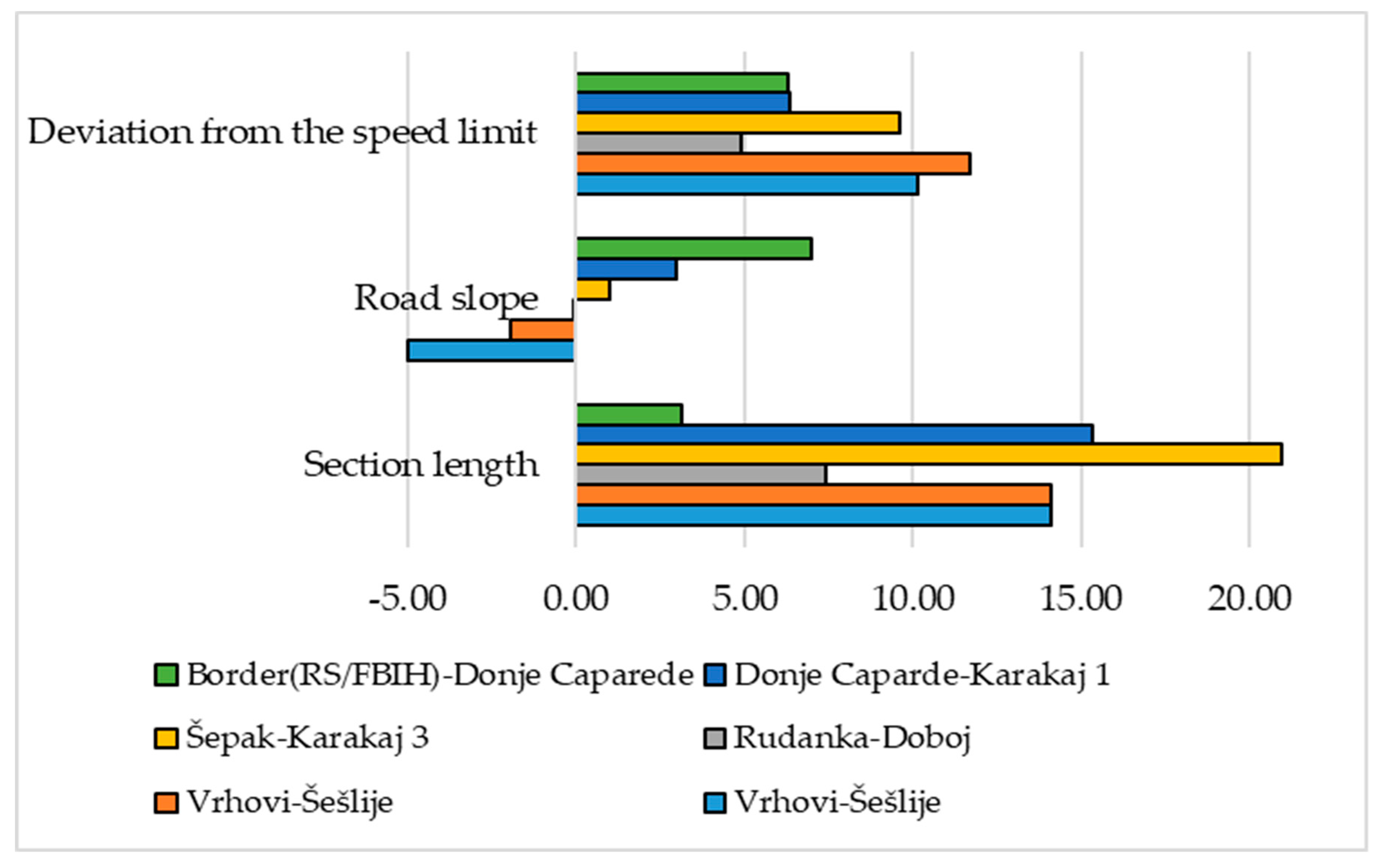
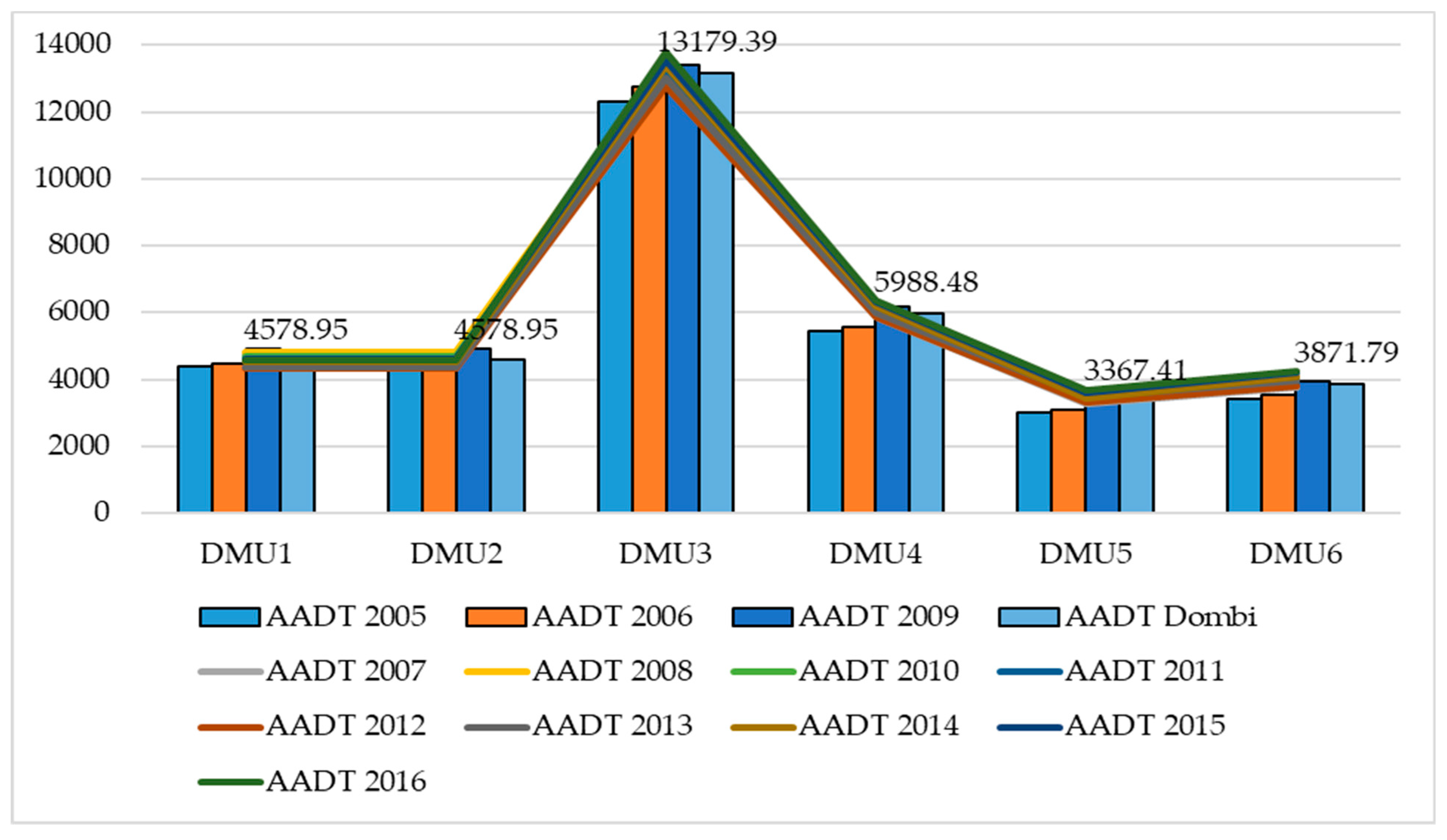
In the third phase of this research, a sensitivity analysis consisting of three parts was conducted. The first part presents the change of input values through 40 newly formed scenarios in which their weights ware simulated using Equation (28).
W n β = ( 1 W n α ) W β ( 1 W n )
W ˜ n α indicates the reduced value of the input the weight of which changes, W ˜ β indicates the real value of the input considered, while W ˜ n indicates the original value of the input the value of which increases. In the second part of the verification of the results, the ranking reversal problem is applied [46], in which the size of the initial fuzzy matrix is changed. This is followed by a comparative analysis with three other fuzzy MCDM methods: fuzzy WASPAS [47], fuzzy SAW [48], and fuzzy TOPSIS [49].

5. Case Study

5.1. Formation of Input-Output Parameters and Averaging Using Dombi and Bonferroni Aggregators

The input parameters for the given sections are: section length—I1, road slope—I2, deviation from the speed limit—I3, and average annual daily traffic (AADT)—I4. The classifications of traffic accidents with fatalities, severe injuries, minor injuries, and material damage are defined as output parameters, O1, O2, O3, and O4, respectively. These parameters are defined on the basis of the authors’ practical experiences, similar studies, and dialogue with other experts. Table 6 shows the values of all DMUs according to the input-output parameters.
A total of six sections of the road network on the territory of the Republic of Srpska: Vrhovi-Šešlije I, Vrhovi-Šešlije II, Rudanka-Doboj, Šepak-Karakaj 3, Donje Caparde-Karakaj 1, and Border (RS/FBIH)-Donje Caparde, were considered.
Figure 2 shows the lengths of six analyzed sections, the slopes on the measured sections (upgrade/downgrade), and the arithmetic mean of the speed deviation of passenger cars from the speed limit on the measured sections. The measured sections were determined for different values of longitudinal gradients. At 1000 m in front of the measured cross section, the value of the average downgrade/upgrade was determined (−5.00%, −1.92%, −0.017%, + 1.00%, 3.00%, and 7.00%). The largest section length is Šepak-Karakaj 3 (20.95 km), and the smallest is Border (RS-FBIH)-Donje Caparde (3.14 km). The sections Vrhovi-Šešlije and Border (RS-FBIH)-Donje Caparde can be classified as hilly sections according to their terrain configuration. The arithmetic means of deviations from the speed limit were determined on the measured sections. The credibility of the speed limit on the section Vrhovi-Šešlije for both values of the measured longitudinal downgrades is especially endangered, with exceedances of over 10 km/h. In this case, the speeding of passenger cars as representative vehicles was analyzed, and it was determined that the credibility of the speed limit was significantly endangered for the downgrade. Additionally, with the increase of the ascent on the measured sections, a deviation from the speed limit which did not endanger the credibility of the speed limit was determined.
Figure 3 shows the AADT values for the available period of 12 years, from 2005 to 2016, where the value of AADT on the plain section Rudanka-Doboj deviates significantly (0.017% ≈ 0.00%), while, on the other five sections, the arithmetic mean of AADT does not exceed the value of 6000 vehicles/day, except at the section Rudanka-Doboj, where the AADT is 13,179.39 vehicles/day. On all sections, the slight increase/decrease of AADT by years is not balanced.
Figure 4 shows the average number of traffic accidents in the period from 2015 to 2019 by the type of accident and the specified sections. Figure 4 shows the total number of traffic accidents, with the section DMU3, Rudanka-Doboj, standing out negatively, considering that there are also accidents with fatalities in the period from 2015 to 2019. On average, 1.4 persons were killed annually on this section. When observing the stated time period, the number of traffic accidents with fatalities is 2, 2, 1, 1, and 1, respectively. Additionally, on the section DMU4, Šepak 3-Karakaj, 1.4 persons were killed annually, with the number of fatalities by years 2, 1, 1, 2, and 1, respectively. On average, 53.40 traffic accidents with material damage occurred on the same section in five years, making this section especially risky. The lowest number of accidents was recorded on the shortest section DMU6, Border (RS-BIH)-Donje Caparde, where in the period of five analyzed years, the number of total accidents per year does not exceed five, and there are no fatalities on this section. These indicators of the number of accidents per year were analyzed and used in further data synthesis. It is clearly noticeable that DMU4 and DMU3 stand out in terms of the number of traffic accidents by all classes.
In order to obtain the final data that will represent the input, i.e., output of the DEA model, it is necessary to use the Dombi aggregator for averaging the historical data for the AADT as inputs, and the Bonferroni aggregator for averaging all outputs of the DEA model. An example of the application of both aggregators and the averaging of the stated values is shown below. The AADT values for the first and second DMU are obtained using a Dombi aggregator as follows:
( b 1 ) = j = 1 n ( b 1 ) 1 + ( j = 1 n w j ( 1 f ( b j ) f ( b j ) ) ) = 55033 1 + ( 1 12 ( 1 0.0795 0.0795 ) + 1 12 ( 1 0.081 0.081 ) + + 1 12 ( 1 0.083 0.083 ) ) = 55033 12.019 = 4578.95 f ( b 1 ) = 4375 4375 + 4470 + 4782 + 4829 + 4931 + 4676 + 4547 + 4334 + 4366 + 4548 + 4600 + 4575 = 4375 55033 = 0.0795
All AADT values shown in Figure 3 were obtained in the same way.
The values of all outputs are obtained using the Bonferroni aggregator as follows.
For the first DMU1 for the first output O1traffic accidents with fatalities:
B M p = 1 , q = 1 = ( 2 , 0 , 2 , 0 , 0 ) = ϖ D M U 1 ( 1 ) = ( 1 5 ( 5 1 ) i , j = 1 i j 5 ϖ D M U 1 ( 1 ) i ϖ D M U 1 ( 1 ) j ) 1 1 + 1 = ( 0.050 ( 2 1 0 1 + 2 1 2 1 + 2 1 0 1 + 2 1 0 1 + 0 1 2 1 + 0 1 2 1 + 0 1 0 1 + 0 1 0 1 + + 0 1 2 1 + 0 1 0 1 + 0 1 2 1 + 0 1 0 1 ) ) 1 1 + 1 = 0.632
In this research, e represents the year number for traffic accidents, which means individually each year in the interval 20152019, while p, q ≥ 0 are a set of non-negative numbers. In the same way, averaged values are obtained for all outputs shown in Figure 4.

5.2. Determination of Weight Values Using the Improved Fuzzy SWARA (IMF SWARA) Method

In the previous section of the paper, the validity of the developed IMF SWARA method was proved, so the results of weight coefficients for the criteria, i.e., the inputs and outputs of the considered study, are presented below. The weight coefficients of the criteria obtained using the IMF SWARA method are shown in Table 7.
The most significant criterion from the set of observed criteria is O1 with a value of 0.213, which represents the number of traffic accidents with fatalities. According to this criterion, the prominent sections, DMU3 and DMU4, are evaluated especially negatively. Additionally, a significant influential criterion is the number of accidents with severe injuries, O2, and the deviation from the speed limit, I3, with a value of 0.170. The values of the input parameters in a small range are slightly higher compared to the less significant ones. Compared to other inputs, there is no input with a significantly higher advantage.

5.3. Application of DEA Model

Further in the paper, the DEA output-oriented model is presented in order to determine the sections of two-lane roads, i.e., DMUs, which show a rather satisfactory safety degree in a certain manner. It is these sections that are implemented further into the model and ranked using the fuzzy MARCOS method. The DEA algorithms are defined and solved using the Lingo 17 software, an example of which is given below (DMU1).
D E A o u p u t D M U 1 = MIN = 0.63 w 5 + 2.49 w 6 + 3.7 w 7 + 7.26 w 8 ; 14.07 w 1 5.00 w 2 10.16 w 3 4578.95 w 4 + ( 0.63 w 5 + 2.49 w 6 + 3.7 w 7 + 7.26 w 8 ) > = 0 ; 14.07 w 1 1.92 w 2 11.67 w 3 4578.95 w 4 + ( 0.63 w 5 + 2.49 w 6 + 3.7 w 7 + 7.26 w 8 ) > = 0 ; 7.41 w 1 0.02 w 2 4.88 w 3 13179.39 w 4 + ( 1.38 w 5 + 4.81 w 6 + 14.42 w 7 + 49.72 w 8 ) > = 0 ; 20.95 w 1 1.00 w 2 9.61 w 3 5988.48 w 4 + ( 1.38 w 5 + 5.67 w 6 + 19.38 w 7 + 53.18 w 8 ) > = 0 ; 15.35 w 1 3.00 w 2 6.33 w 3 3367.41 w 4 + ( 0.55 w 5 + 3.16 w 6 + 6.26 w 7 + 21.09 w 8 ) > = 0 ; 3.14 w 1 7.00 w 2 6.29 w 3 3871.79 w 4 + ( 0.00 w 5 + 0.32 w 6 + 0.84 w 7 + 1.95 w 8 ) > = 0 ; 14.07 w 1 + 5.00 w 2 + 10.16 w 3 + 4578.95 w 4 = 1 ; w 1 > 0 ; w 2 > 0 ; w 3 > 0 ; w 4 > 0 ; w 5 > 0 ; w 6 > 0 ; w 7 > 0 ; w 8 > 0 ;
After solving the set algorithm, the objective function is 1.000. After that, the algorithms for the other DMUs according to inputs are formed. Regardless of the fact that it is not necessary to perform the calculation using both models (input and output), the output-oriented model is performed for internal calculation control in this study. The final results using the DEA model are shown in Table 8.
Road sections marked DMU1, DMU2, and DMU6 with a displayed value of 1.000 are further implemented in the model and ranked using the fuzzy MARCOS method. Other sections, DMU3, DMU4, and DMU5, with the values of 19.540, 7.064, and 2.362, respectively, are eliminated further from the model because they show an inadequate safety degree and a corrective action in the implementation of certain measures is necessary.

5.4. Application of the Fuzzy MARCOS Method in Order to Make Final Ranking of Road Sections

In the previous section of the paper, the DEA model was applied, and it was determined which road sections should be included further in the model. Additionally, the initial fuzzy decision matrix was defined on the basis of the scale shown in Table 9.
Taking into account the given linguistic scale, the initial fuzzy decision matrix was formed, after which Equations (14) and (15) were applied in order to determine ideal and anti-ideal solutions. The extended fuzzy initial matrix is shown in Table 10, and it is important to note that criteria C1, C2, and C4 are beneficial and thus for whom the maximum value is desired, while the others belong to the group of cost criteria with the preference of the minimum value.
The next step involves performing the normalization of the matrix shown in Table 10, taking into account the type of criteria. Equation (16) is applied to the cost group of criteria as follows: n ˜ 13 = ( 1.000 5.000 , 1.000 5.000 , 1.000 3.000 ) = ( 0.200 , 0.200 , 0.333 ) , while for the group of criteria that prefer the maximum value, Equation (17) is applied: n ˜ 11 = ( 7.000 9.000 , 9.000 9.000 , 9.000 9.000 ) = ( 0.778 , 1.000 , 1.000 ) . The complete fuzzy normalized matrix is shown in Table 11.
In the next step, the previous matrix is weighted by multiplying the values from Table 11 by the weight coefficients obtained using the IMF SWARA method by Equation (18) as follows:
v ˜ 11 = ( n 11 l × w 1 l , n 11 m × w 1 m , n 11 u × w 1 u ) = ( 0.778 × 0.213 , 1.000 × 0.213 , 1.000 × 0.213 ) = ( 0.166 , 0.213 , 0.213 )
The complete weighted fuzzy matrix is given in Table 12.
The fuzzy matrix S ˜ i is obtained by applying Equation (19),
S ˜ a i = ( 0.226 , 0.350 , 0.388 ) , S ˜ 1 = ( 0.454 , 0.606 , 0.629 ) S ˜ 2 = ( 0.406 , 0.531 , 0.569 ) , S ˜ 6 = ( 0.392 , 0.742 , 0.821 ) , S ˜ i d = ( 0.573 , 0.923 , 1.002 )
as follows:
S ˜ a i = ( 0.024 + 0.057 + 0.024 + 0.058 + 0.021 + 0.012 + 0.009 + 0.021 0.071 + 0.057 + 0.034 + 0.097 + 0.035 + 0.016 + 0.012 + 0.027 0.071 + 0.095 + 0.034 + 0.097 + 0.035 + 0.016 + 0.012 + 0.027 ) = ( 0.226 , 0.350 , 0.388 )
Using Equation (20), the matrix K ˜ i is obtained,
k ˜ 1 = ( 1.171 , 1.734 , 2.789 ) k ˜ 2 = ( 1.049 , 1.517 , 2.521 ) k ˜ 6 = ( 1.011 , 2.121 , 3.640 )
as follows:
k ˜ 1 = S ˜ 1 S ˜ a i = ( s 1 l s a i u , s 1 m s a i m , s 1 u s a i l ) = ( 0.454 0.388 , 0.606 0.350 , 0.629 0.226 ) = ( 1.171 , 1.734 , 2.789 )
Using Equation (21), the matrix K ˜ i + is obtained,
k ˜ 1 + = ( 0.453 , 0.657 , 1.098 ) k ˜ 2 + = ( 0.406 , 0.575 , 0.993 ) k ˜ 6 + = ( 0.391 , 0.804 , 1.434 )
as follows:
k ˜ 1 + = S ˜ 1 S ˜ i d = ( s 1 l s i d u , s 1 m s i d m , s 1 u s i d l ) = ( 0.454 1.002 , 0.606 0.923 , 0.629 0.573 ) = ( 0.453 , 0.657 , 1.098 )
The matrix T ˜ i is calculated using Equation (22):
t ˜ 1 = ( 1.624 , 2.391 , 3.888 ) , t ˜ 2 = ( 1.454 , 2.092 , 3.513 ) , t ˜ 6 = ( 1.402 , 2.925 , 5.073 )
in the following way:
t ˜ 1 = ( 1.171 + 0.453 , 1.734 + 0.657 , 2.789 + 1.098 ) = ( 1.624 , 2.391 , 3.888 )
After that, a fuzzy number D ˜ = ( 1.624 , 2.925 , 5.073 ) using Equation (23) is calculated. Defuzzification is done by Equation (24) obtaining the number d f c r i s p = 3.066 . The final results calculated using the fuzzy MARCOS method are shown in Table 13.
Utility functions f ( K ˜ i + ) and f ( K ˜ i ) are calculated applying Equations (25) and (26).
f ( K ˜ 1 + ) = K ˜ 1 d f c r i s p = ( 1.171 3.066 , 1.734 3.066 , 2.789 3.066 ) ,   f ( K ˜ 1 ) = K ˜ 1 + d f c r i s p = ( 0.453 3.066 , 0.657 3.066 , 1.098 3.066 )
Then defuzzification if performed for K ˜ i , K ˜ i + , f ( K ˜ i + ) , f ( K ˜ i ) . The calculation of the utility function of alternatives f K i is obtained using Equation (27).
f ( K 1 ) = K 1 + + K 1 1 + 1 f ( K 1 + ) f ( K 1 + ) + 1 f ( K 1 ) f ( K 1 ) = 0.453 + 1.171 1 + 1 0.382 0.382 + 1 0.148 0.148 = 0.494
After applying the integrated DEA—IMF SWARA—fuzzy MARCOS methodology based on the application of Dombi and Bonferroni aggregators, the final results are obtained. The section of the two-lane road DMU6 Border (RS-FBIH)-Donje Caparde is ranked with the highest level of traffic safety functionally dependent on the technical and exploitation indicators of the road network. The value of the rank size is 0.748, while the other two sections, DMU1 and DMU2, have incomparably lower values of 0.494 and 0.378, which shows a higher traffic risk on the measured parts of these sections.

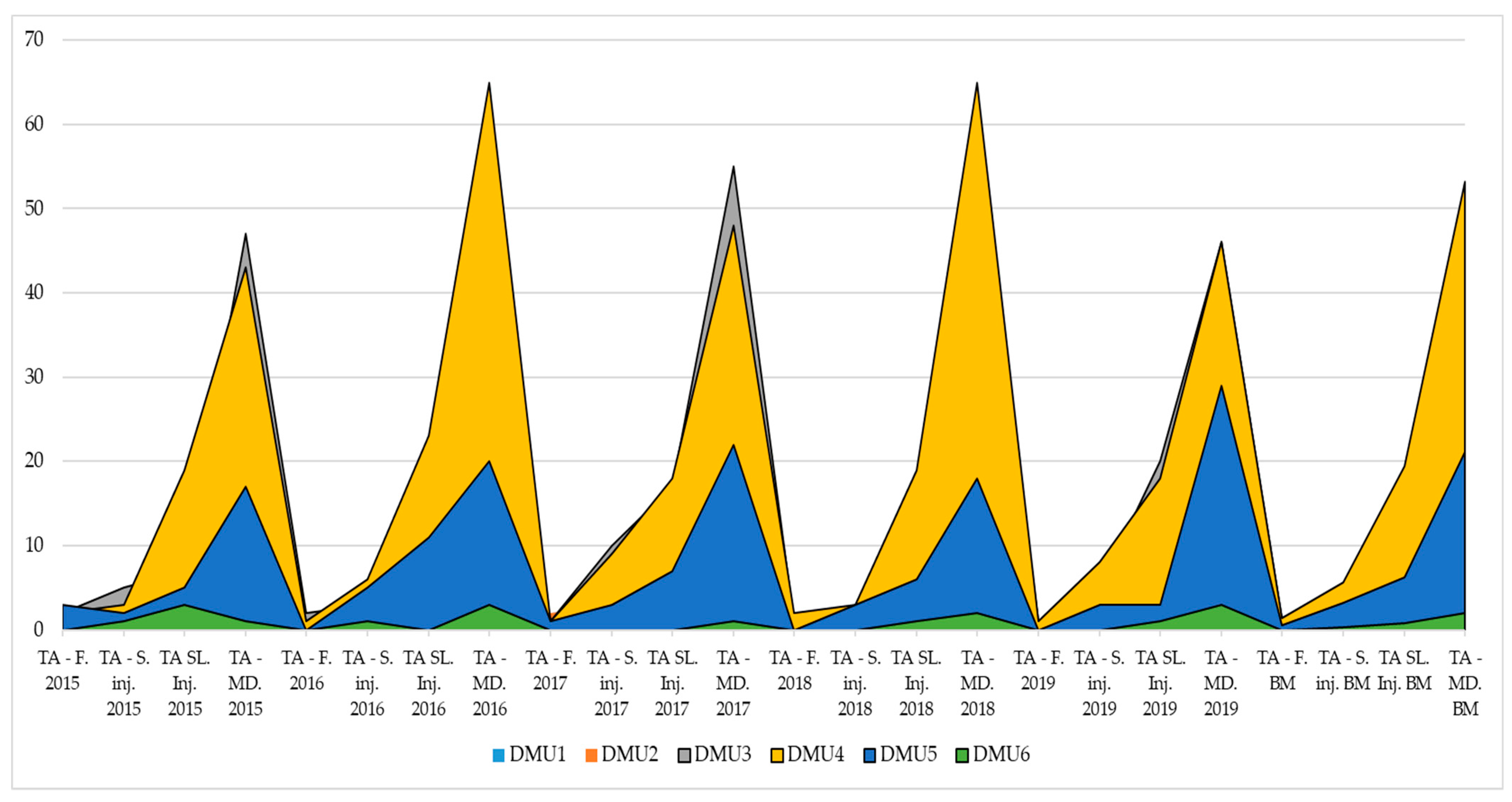
6. Sensitivity Analysis

6.1. Testing the Change in Weights of Inputs

One way to test the sensitivity of the model is to simulate the weight coefficients of the criteria by applying the aforementioned Equation (28). It is important to note that a total of 40 new scenarios were formed in which the value of the input was simulated through 10 scenarios individually. In the first 10 scenarios, the value of the first input C1 was reduced by 10% for each scenario, meaning that in scenario S10, the first input had no significance, i.e., the value was zero. The other 30 scenarios for criteria C2, C3, and C4 were formed in the same way. Thus, the input values were corrected in the range of 10–100%. The values of input weight coefficients through the newly formed 40 scenarios are given in Figure 5.
Each scenario was observed separately, so recalculation was performed with the fuzzy MARCOS method and new results were obtained that confirmed the original rank. Thus, there is no change in any rank, while the final values of the DMUs certainly change. In the first 10 scenarios where the significance of the first input is reduced, the value of the best DMU6 increases, while the other two decrease. The same is the case with the change in the influence of the fourth input, i.e., in scenarios S31–S40. When the value of the second input changes, the value of the best-ranked DMU6 decreases, while the value of DMU2 increases and approaches DMU1. As the value of the third input changes, the value of DMU6 decreases, and the other two increase, with DMU1 approaching DMU6. This means that the model is completely insensitive to changes in input significance.

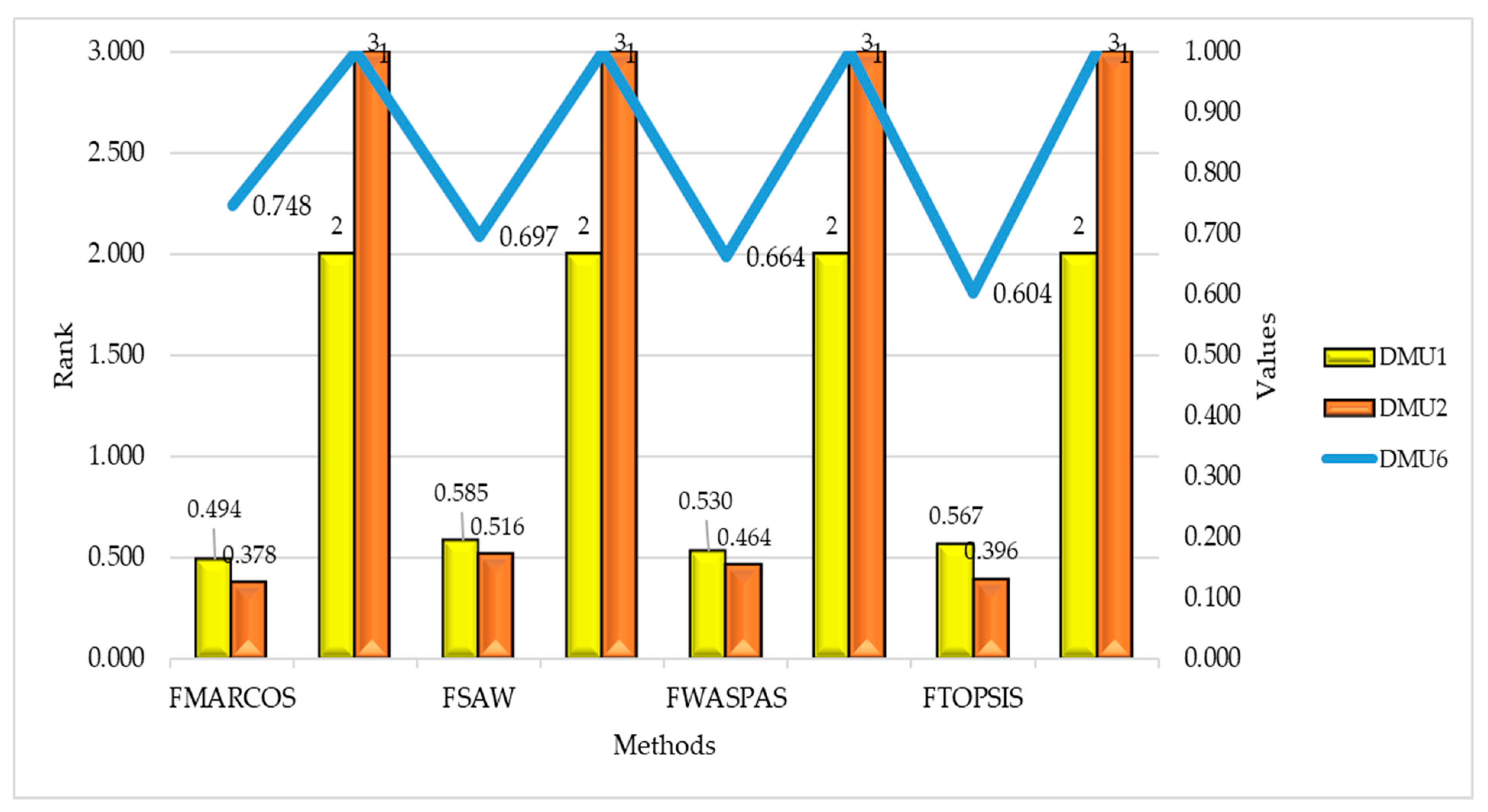
6.2. Comparison with Other MCDM Methods in a Fuzzy Form

As a second part of this analysis, a comparative analysis with three other methods in a fuzzy form was performed, as explained in detail in the third phase of the methodology section. Figure 6 shows the values and ranks of the DMUs using the fuzzy SAW, fuzzy WASPAS, and fuzzy TOPSIS methods.
Figure 6 shows that the ranks are fully correlated with the initial rank obtained by applying the integrated IMF SWARA—fuzzy MARCOS model. In addition to the ranks, the values of all DMUs are shown in order to provide a better insight into the comparative analysis. Once again, the stability of the model and the more precise data obtained with the fuzzy MARCOS method can be proven through the observation of the intervals of all values using all methods.

6.3. Influence of Dynamic Initial Matrix Formation

Figure 7 shows the results after applying the sensitivity analysis related to the change in the size of the initial fuzzy matrix. Two new scenarios have been defined in which the sizes of the initial matrix are changed in such a way that the worst-ranked alternative is eliminated from the initial matrix.
Observing the results in Figure 7, was can see that the change in the size of the fuzzy initial matrix has absolutely no effect on the rankings, as the rankings do not change in either of the two scenarios formed.

7. Conclusions

Through this study we defined a new integrated fuzzy model that combines several different approaches in the field of decision making, and a combination of this with the DEA model for initial determination of road section safety based on the geometric exploitation of road parameters: section length, road slope, speed deviation from the speed limit, and AADT as input parameters. The output parameters in the DEA model represent different classifications of traffic accidents. The overall research was previously presented in detail through three phases. The greatest contributions of this research can be observed from two aspects: scientific and professional. From a scientific aspect, the main, and probably the most important contribution, is the development of the improved fuzzy SWARA method (IMF SWARA), overcomes the disadvantages of the fuzzy SWARA method in the following ways:
(1)
Using the fuzzy SWARA method, it is impossible to obtain results in which two criteria have equal fuzzy weights. By applying the improved fuzzy SWARA method, two or more criteria can have equal values.
(2)
On the contrary, applying the inadequate TFN scale shown in Table 2, where decision-makers indicate that two criteria have the same value by assigning TFN (1,1,1), the criterion Cj in relation to Cj−1 received a value that is twice less than Cj. By applying the improved fuzzy SWARA method, assigning the value (0,0,0), equal values are obtained and not values twice as large.
(3)
By increasing the number of criteria in the model, the least significant criteria receive values that can be negligible, i.e., with a tendency to zero. By applying the improved fuzzy SWARA method, less significant criteria have higher values and can play a greater role in the decision-making process.
Then, the integration of the developed IMF SWARA method with the fuzzy MARCOS method was performed, which is also a contribution of this paper. In order to achieve greater precision in the creation of input data, the originality of the given model was manifested by the application of two aggregators: Dombi and Bonferroni, which were used to average the input-output parameters. The creation and verification of such a model certainly represents a contribution to the overall literature that considers multi-criteria problems. If we take into account that according to Salabun et. al. [50] in many studies, the problem of selecting the proper method and parameters for decision-making is raised, we can conclude that our integrated fuzzy model represents a good solution. This has been proved through the aforementioned scientific contributions of the developed model.
From a professional perspective, the contribution of this research is reflected through the quantification of the safety degree of certain sections of road infrastructure, which is an important parameter in practice. Taking into account the previously stated parameters with a focus on passenger cars exceeding the speed limit, the road sections from the considered set that represent risk have been defined, indicating that a corrective measure in traffic management is necessary.
The limitations of this study can be manifested through the small number of considered road sections and the inclusion of input/output parameters without the performance principal component analysis. The results calculated using the original IMF SWARA–Fuzzy MARCOS model indicate that the sixth section of the observed two-lane roads shows the highest level of traffic safety with a value of 0.748, taking into account the complexity of the set model. The next section is the DMU2 with a value of 0.494, and in the third position is section DMU2, while the remaining three sections, DMU3, DMU4, and DMU5, have a higher risk of side effects, i.e., traffic accidents. After applying the original IMF SWARA—Fuzzy MARCOS model, a sensitivity analysis was performed, through which the overall stability of the model was proven.
Future research may need to be conducted on a number of road sections with the possibility of implementing the proposed model. The existing model, with an increase of input parameters, could contribute to a much more selective level of choosing the rank of road sections. It is also possible for the number of access points on each section, the radius of the road, etc., to be added as input parameters. Additionally, by applying the existing model through observing other input parameters, an extensive analysis in ranking the safety level of the two-lane roads in terms of multi-criteria traffic analysis can be obtained. Besides, a PCA–DEA analysis [51] can be applied to determine the efficiency of the considered road sections or to implement the group MCDM model [52] along with some different uncertainty theories such multi-granular unbalanced linguistic information [53], intuitionistic 2-tuple linguistic sets [54], or grey theory [55]. Considering the approach presented in [56] can be useful in developing future integrated decision-making models.

Author Contributions

Conceptualization, S.V. and E.S.; methodology, Ž.S. and M.S.; formal analysis, M.S. and M.P.; data curation, M.S. and E.S.; writing—original draft preparation, Ž.S. and S.V.; writing—review and editing, M.D. and M.P.; supervision, M.D. and M.P.; All authors have read and agreed to the published version of the manuscript.

Funding

This research received no external funding.

Informed Consent Statement

Not applicable.

Data Availability Statement

Not applicable.

Conflicts of Interest

The authors declare no conflict of interest.

References

  1. Mayora, J.P.; Rubio, R.L. Relevant Variables for Crash Rate Prediction in Spain´s Two Lane Rural Roads. In Proceedings of the 82nd Transportation Research Board Annual Meeting, Washington, DC, USA, 12–16 January 2003. [Google Scholar]
  2. Qiao, J.; Wen, Y.; Yang, N.; Song, J. The research of two-lane highway longitudinal slope based on the running speed in the plateau areas. In Proceedings of the 2011 International Conference on Consumer Electronics, Communications and Networks (CECNet), Xianning, China, 16–18 April 2011; pp. 1827–1830. [Google Scholar] [CrossRef]
  3. Hashim, I.H. Analysis of speed characteristics for rural two-lane roads: A field study from Minoufiya Governorate, Egypt. Ain Shams Eng. J. 2011, 2, 43–52. [Google Scholar] [CrossRef] [Green Version]
  4. D’Andrea, A.; Carbone, F.; Salviera, S.; Pellegrino, O. The Most Influential Variables in the Determination of V85 Speed. Procedia Soc. Behav. Sci. 2012, 53, 633–644. [Google Scholar] [CrossRef] [Green Version]
  5. Porter, R.J.; Donnell, E.T.; Mason, J.M. Geometric Design, Speed, and Safety. Transp. Res. Rec. 2012, 2309, 39–47. [Google Scholar] [CrossRef]
  6. Highway Capacity Manual 2016 (HCM 2016); TRB. National Research Council: Washington, DC, USA, 2016.
  7. Handbuch für die Bemessung von Straßenverkehrsanlagen (HBS) (German Highway Capacity Manual); Forschungsgesellschaft für Straßen-und Verkehrswesen: Köln, Germany, 2005.
  8. AASHTO. The Highway Safety Manual; American Association of State Highway Transportation Professionals: Washington, DC, USA, 2010. [Google Scholar]
  9. Aarts, L.; van Schagen, I. Driving speed and the risk of road crashes: A review. Accid. Anal. Prev. 2006, 38, 215–224. [Google Scholar] [CrossRef] [PubMed]
  10. Cruzado, I.; Donnell, E.T. Factors Affecting Driver Speed Choice along Two-Lane Rural Highway Transition Zones. J. Transp. Eng. 2010, 136, 755–764. [Google Scholar] [CrossRef] [Green Version]
  11. Cheng, G.; Cheng, R.; Pei, Y.; Xu, L. Probability of Roadside Accidents for Curved Sections on Highways. Math. Probl. Eng. 2020, 2020, 1–18. [Google Scholar] [CrossRef]
  12. Zheng, Y.; Guo, H.; Wei, X. The Evaluation Analysis of Design Code About the Road Design of longitudinal gradient in the Mountain Road. In Proceedings of the 7th International Conference on Education, Management, Computer and Society (EMCS 2017), Shenyang, China, 17–19 March 2017; pp. 693–699. [Google Scholar] [CrossRef] [Green Version]
  13. Srnová, B. A Case of Road Design in Mountainous Terrain with an Evaluation of Heavy Vehicles Performance Stockholm. Master’s Thesis, KTH Royal Institute of Technology, Stockholm, Sweden, 2017. [Google Scholar]
  14. Fitzpatrick, K.; Schneider, W.H.; Park, E.S. Comparisons of Crashes on Rural Two-Lane and Four-Lane Highways in Texas; FHWA/TX-06/0-4618-1; Report 0-4618-1; Texas Transportation Institute: Bryan, TX, USA, 2005. [Google Scholar]
  15. Calvo-Poyo, F.; de Oña, J.; Garach Morcillo, L.; Navarro-Moreno, J. Influence of Wider Longitudinal Road Markings on Vehicle Speeds in Two-Lane Rural Highways. Sustainability 2020, 12, 8305. [Google Scholar] [CrossRef]
  16. Yue, L.; Wang, H. An Optimization Design Method of Combination of Steep Slope and Sharp Curve Sections for Mountain Highways. Math. Probl. Eng. 2019, 2019, 1–13. [Google Scholar] [CrossRef] [Green Version]
  17. Kazemzadehazad, S.; Monajjem, S.; Larue, G.; King, M.J. Driving simulator validation for speed research on curves of two-lane rural roads. In Proceedings of the Institution of Civil Engineers—Transport; Thomas Telford Ltd.: London, UK, 2018; pp. 1–18. [Google Scholar] [CrossRef]
  18. Abdollahzadeh Nasiri, A.S.; Rahmani, O.; Abdi Kordani, A.; Karballaeezadeh, N.; Mosavi, A. Evaluation of Safety in Horizontal Curves of Roads Using a Multi-Body Dynamic Simulation Process. Int. J. Environ. Res. Public Health 2020, 17, 5975. [Google Scholar] [CrossRef]
  19. Khabiri, M.M.; Ghaforifard, Z. The Effect of Low Friction in Pavement Due to Floods and High-speed Vehicles in Increasing the Number of Rescue Vehicles’ Driving Accidents. Health Emerg. Disasters 2020, 6, 29–38. [Google Scholar] [CrossRef]
  20. Sil, G.; Maji, A.; Nama, S.; Maurya, A.K. Operating speed prediction model as a tool for consistency based geometric design of four-lane divided highways. Transport 2019, 34, 425–436. [Google Scholar] [CrossRef] [Green Version]
  21. Alper, D.; Sinuany-Stern, Z.; Shinar, D. Evaluating the efficiency of local municipalities in providing traffic safety using the Data Envelopment Analysis. Accid. Anal. Prev. 2015, 78, 39–50. [Google Scholar] [CrossRef]
  22. Podvezko, V.; Sivilevičius, H. The use of AHP and rank correlation methods for determining the significance of the interaction between the elements of a transport system having a strong influence on traffic safety. Transport 2013, 28, 389–403. [Google Scholar] [CrossRef]
  23. Pirdavani, A.; Brijs, T.; Wets, G. A Multiple Criteria Decision-Making Approach for Prioritizing Accident Hotspots in the Absence of Crash Data. Transp. Rev. 2010, 30, 97–113. [Google Scholar] [CrossRef]
  24. Barić, D.; Pilko, H.; Strujić, J. An analytic hierarchy process model to evaluate road section design. Transport 2016, 31, 312–321. [Google Scholar] [CrossRef] [Green Version]
  25. Pilko, H.; Mandžuka, S.; Barić, D. Urban single-lane roundabouts: A new analytical approach using multi-criteria and simultaneous multi-objective optimization of geometry design, efficiency and safety. Transp. Res. Part C Emerg. Technol. 2017, 80, 257–271. [Google Scholar] [CrossRef]
  26. Zak, J. The methodology of multiple criteria decision making/aiding in public transportation. J. Adv. Transp. 2010, 45, 1–20. [Google Scholar] [CrossRef]
  27. Krstić, M.D.; Tadić, S.R.; Brnjac, N.; Zečević, S. Intermodal Terminal Handling Equipment Selection Using a Fuzzy Multi-criteria Decision-making Model. Promet Traffic Transp. 2019, 31, 89–100. [Google Scholar] [CrossRef]
  28. Vakilipour, S.; Sadeghi-Niaraki, A.; Ghodousi, M.; Choi, S.-M. Comparison between Multi-Criteria Decision-Making Methods and Evaluating the Quality of Life at Different Spatial Levels. Sustainability 2021, 13, 4067. [Google Scholar] [CrossRef]
  29. Yannis, G.; Kopsacheili, A.; Dragomanovits, A.; Petraki, V. State-of-the-art review on multi-criteria decision-making in the transport sector. J. Traffic Transp. Eng. (Engl. Ed.) 2020, 7, 413–431. [Google Scholar] [CrossRef]
  30. Memiş, S.; Demir, E.; Karamaşa, Ç.; Korucuk, S. Prioritization of road transportation risks: An application in Giresun province. Oper. Res. Eng. Sci. Theory Appl. 2020, 3, 111–126. [Google Scholar] [CrossRef]
  31. Đalić, I.; Ateljević, J.; Stević, Ž.; Terzić, S. An integrated swot–fuzzy piprecia model for analysis of competitiveness in order to improve logistics performances. Facta Univ. Ser. Mech. Eng. 2020, 18, 439–451. [Google Scholar]
  32. Vesković, S.; Milinković, S.; Abramović, B.; Ljubaj, I. Determining criteria significance in selecting reach stackers by applying the fuzzy PIPRECIA method. Oper. Res. Eng. Sci. Theory Appl. 2020, 3, 72–88. [Google Scholar] [CrossRef]
  33. Pamucar, D. Normalized weighted Geometric Dombi Bonferoni Mean Operator with interval grey numbers: Application in multicriteria decision making. Rep. Mech. Eng. 2020, 1, 44–52. [Google Scholar] [CrossRef]
  34. Yager, R.R. On generalized Bonferroni mean operators for multi-criteria aggregation. Int. J. Approx. Reason. 2009, 50, 1279–1286. [Google Scholar] [CrossRef] [Green Version]
  35. Mavi, R.K.; Goh, M.; Zarbakhshnia, N. Sustainable third-party reverse logistic provider selection with fuzzy SWARA and fuzzy MOORA in plastic industry. Int. J. Adv. Manuf. Technol. 2017, 91, 2401–2418. [Google Scholar] [CrossRef]
  36. Chang, D.Y. Applications of the extent analysis method on fuzzy AHP. Eur. J. Oper. Res. 1996, 95, 649–655. [Google Scholar] [CrossRef]
  37. Zarbakhshnia, N.; Soleimani, H.; Ghaderi, H. Sustainable third-party reverse logistics provider evaluation and selection using fuzzy SWARA and developed fuzzy COPRAS in the presence of risk criteria. Appl. Soft Comput. 2018, 65, 307–319. [Google Scholar] [CrossRef]
  38. Ulutaş, A.; Karakuş, C.B.; Topal, A. Location selection for logistics center with fuzzy SWARA and CoCoSo methods. J. Intell. Fuzzy Syst. 2020, 38, 4693–4709. [Google Scholar] [CrossRef]
  39. Ansari, Z.N.; Kant, R.; Shankar, R. Evaluation and ranking of solutions to mitigate sustainable remanufacturing supply chain risks: A hybrid fuzzy SWARA-fuzzy COPRAS framework approach. Int. J. Sustain. Eng. 2020, 13, 473–494. [Google Scholar] [CrossRef]
  40. Ghasemi, P.; Mehdiabadi, A.; Spulbar, C.; Birau, R. Ranking of Sustainable Medical Tourism Destinations in Iran: An Integrated Approach Using Fuzzy SWARA-PROMETHEE. Sustainability 2021, 13, 683. [Google Scholar] [CrossRef]
  41. Mitrović Simić, J.; Stević, Ž.; Zavadskas, E.K.; Bogdanović, V.; Subotić, M.; Mardani, A. A Novel CRITIC-Fuzzy FUCOM-DEA-Fuzzy MARCOS Model for Safety Evaluation of Road Sections Based on Geometric Parameters of Road. Symmetry 2020, 12, 2006. [Google Scholar] [CrossRef]
  42. Blagojević, A.; Vesković, S.; Kasalica, S.; Gojić, A.; Allamani, A. The application of the fuzzy AHP and DEA for measuring the efficiency of freight transport railway undertakings. Oper. Res. Eng. Sci. Theory Appl. 2020, 3, 1–23. [Google Scholar] [CrossRef]
  43. Andrejić, M.; Kilibarda, M.; Pajić, V. Measuring efficiency change in time applying malmquist productivity index: A case of distribution centres in Sserbia. Facta Univ. Ser. Mech. Eng. 2021. [Google Scholar]
  44. Stanković, M.; Stević, Ž.; Das, D.K.; Subotić, M.; Pamučar, D. A new fuzzy MARCOS method for road traffic risk analysis. Mathematics 2020, 8, 457. [Google Scholar] [CrossRef] [Green Version]
  45. Bakır, M.; Atalık, Ö. Application of Fuzzy AHP and Fuzzy MARCOS Approach for the Evaluation of E-Service Quality in the Airline Industry. Decis. Mak. Appl. Manag. Eng. 2021, 4, 127–152. [Google Scholar] [CrossRef]
  46. Zahir, S. Normalisation and rank reversals in the additive analytic hierarchy process: A new analysis. Int. J. Oper. Res. 2009, 4, 446–467. [Google Scholar] [CrossRef]
  47. Petrović, G.; Mihajlović, J.; Ćojbašić, Ž.; Madić, M.; Marinković, D. Comparison of three fuzzy MCDM methods for solving the supplier selection problem. Facta Univ. Ser. Mech. Eng. 2019, 17, 455–469. [Google Scholar] [CrossRef]
  48. Roszkowska, E.; Kacprzak, D. The fuzzy saw and fuzzy TOPSIS procedures based on ordered fuzzy numbers. Inf. Sci. 2016, 369, 564–584. [Google Scholar] [CrossRef]
  49. Hassanpour, M. Evaluation of Iranian wood and cellulose industries. Decis. Mak. Appl. Manag. Eng. 2019, 2, 13–34. [Google Scholar] [CrossRef]
  50. Sałabun, W.; Wątróbski, J.; Shekhovtsov, A. Are MCDA Methods Benchmarkable? A Comparative Study of TOPSIS, VIKOR, COPRAS, and PROMETHEE II Methods. Symmetry 2020, 12, 1549. [Google Scholar] [CrossRef]
  51. Andrejić, M.M.; Kilibarda, M.J. Measuring global logistics efficiency using PCA-DEA approach. Tehnika 2016, 71, 733–740. [Google Scholar] [CrossRef]
  52. Zhang, Z.; Gao, Y.; Li, Z. Consensus reaching for social network group decision making by considering leadership and bounded confidence. Knowl. Based Syst. 2020, 204, 106240. [Google Scholar] [CrossRef]
  53. Zhang, Z.; Li, Z.; Gao, Y. Consensus reaching for group decision making with multi-granular unbalanced linguistic information: A bounded confidence and minimum adjustment-based approach. Inf. Fusion 2021, 74, 96–110. [Google Scholar] [CrossRef]
  54. Faizi, S.; Sałabun, W.; Nawaz, S. Best-Worst method and Hamacher aggregation operations for intuitionistic 2-tuple linguistic sets. Expert Syst. Appl. 2021, 115088. [Google Scholar] [CrossRef]
  55. Badi, I.; Pamucar, D. Supplier selection for steelmaking company by using combined Grey-MARCOS methods. Decis. Mak. Appl. Manag. Eng. 2020, 3, 37–48. [Google Scholar] [CrossRef]
  56. Zhang, Z.; Kou, X.; Yu, W.; Gao, Y. Consistency improvement for fuzzy preference relations with self-confidence: An application in two-sided matching decision making. J. Oper. Res. Soc. 2020, 1–14. [Google Scholar] [CrossRef]
Figure 1. Research flow diagram with the applied methodology.
Axioms 10 00092 g001
Figure 2. Display of the section length, road slope, and deviation from the speed limit.
Axioms 10 00092 g002
Figure 3. AADT for the period 2005–2016.
Axioms 10 00092 g003
Figure 4. The total number of traffic accidents on all road sections in the period 2015–2019.
Axioms 10 00092 g004
Figure 5. Input weight coefficient values through 40 scenarios.
Axioms 10 00092 g005
Figure 6. Values and ranks of DMUs using the fuzzy SAW, fuzzy WASPAS, and fuzzy TOPSIS methods.
Axioms 10 00092 g006
Figure 7. Results after resizing the fuzzy initial matrix.
Axioms 10 00092 g007
Table 1. New linguistics and the TFN scale for the evaluation of the criteria in the improved fuzzy SWARA (IMF SWARA) method.
Linguistic VariableAbbreviationTFN Scale
Absolutely less significantALS1.0001.0001.000
Dominantly less significantDLS½2/31.000
Much less significantMLS2/51/22/3
Really less significantRLS1/32/51/2
Less significantLS2/71/32/5
Moderately less significantMDLS¼2/71/3
Weakly less significantWLS2/91/42/7
Equally significantES0.0000.0000.000
Table 2. Inadequate scale used by the authors in [35] in fuzzy SWARA.
Linguistic ScaleResponse Scale
Equally important(1, 1, 1)
Moderately less important(2/3, 1, 3/2)
Less important(2/5, 1/2, 2/3)
Very less important(2/7, 1/3, 2/5)
Much less important(2/9, 1/4, 2/7)
Table 3. Calculation process and weights of the main criteria applying fuzzy SWARA in [35].
s j ¯ k j ¯ q j ¯ w j ¯ Crisp Value
C1 1.0001.0001.0001.0001.0001.0000.3770.4050.4440.407
C20.4000.5000.6671.4001.5001.6670.6000.6670.7140.2260.2700.3170.271
C30.2220.2500.2861.2221.2501.2860.4670.5330.5840.1760.2160.2590.217
C40.6671.0001.5001.6672.0002.5000.1870.2670.3510.0700.1080.1560.110
SUM2.2532.4672.649
Table 4. Calculation process and weights of the main criteria applying improved fuzzy SWARA (IMF SWARA) in the same example.
s j ¯ k j ¯ q j ¯ w j ¯ Crisp Value
C1 1.0001.0001.0001.0001.0001.0000.3600.3790.4060.380
C22/71/32/51.2861.3331.4000.7140.7500.7780.2570.2840.3160.285
C32/51/22/31.4001.5001.6670.4290.5000.5560.1540.1890.2250.190
C41/42/71/31.2501.2861.3330.3210.3890.4440.1160.1470.1800.148
SUM2.4642.6392.778
Table 5. Comparative analysis of fuzzy SWARA and improved fuzzy SWARA (IMF SWARA) in another example.
Fuzzy SWARA
s j ¯ k j ¯ q j ¯ w j ¯ Crisp Value
C1 1.0001.0001.0001.0001.0001.0000.2920.3190.3510.320
C20.2860.3330.4001.2861.3331.4000.7140.7500.7780.2090.2390.2730.240
C30.2220.2500.2861.2221.2501.2860.5560.6000.6360.1620.1910.2230.192
C40.4000.5000.6671.4001.5001.6670.3330.4000.4550.0970.1270.1600.128
C50.6671.0001.5001.6672.0002.5000.1330.2000.2730.0390.0640.0960.065
C61.0001.0001.0002.0002.0002.0000.0670.1000.1360.0190.0320.0480.032
C70.6671.0001.5001.6672.0002.5000.0270.0500.0820.0080.0160.0290.017
C80.2860.3330.4001.2861.3331.4000.0190.0380.0640.0060.0120.0220.013
SUM2.8493.1383.423
IMF SWARA
s j ¯ k j ¯ q j ¯ w j ¯ Crisp Value
C1 1.0001.0001.0001.0001.0001.0000.2430.2630.2920.265
C22/71/32/51.2861.3331.4000.7140.7500.7780.1740.1980.2270.199
C32/91/42/71.2221.2501.2860.5560.6000.6360.1350.1580.1860.159
C42/51/22/31.4001.5001.6670.3330.4000.4550.0810.1050.1330.106
C51/42/71/31.2501.2861.3330.2500.3110.3640.0610.0820.1060.082
C60001.0001.0001.0000.2500.3110.3640.0610.0820.1060.082
C71/42/71/31.2501.2861.3330.1880.2420.2910.0460.0640.0850.064
C82/71/32/51.2861.3331.4000.1340.1810.2260.0330.0480.0660.048
SUM3.4253.7964.113
Table 6. Road section parameters in relation to input-output parameters.
I1I2I3I4O1O2O3O4
DMU114.075.0010.164578.950.632.493.707.26
DMU214.071.9211.674578.950.632.493.707.26
DMU37.410.024.8813,179.391.384.8114.4249.72
DMU420.951.009.615988.481.385.6719.3853.18
DMU515.353.006.333367.410.553.166.2621.09
DMU63.147.006.293871.790.000.320.841.95
Table 7. Values of input and output significance in the considered model obtained by applying the IMF SWARA method.
IMF SWARA
s j ¯ k j ¯ q j ¯ w j ¯ Crisp Value
C5 1.0001.0001.0001.0001.0001.0000.2030.2130.2250.213
C62/91/42/71.2221.2501.2860.7780.8000.8180.1580.1700.1840.170
C30.0000.0000.0001.0001.0001.0000.7780.8000.8180.1580.1700.1840.170
C42/91/42/71.2221.2501.2860.6050.6400.6690.1230.1360.1510.136
C11/42/71/31.2501.2861.3330.4540.4980.5360.0920.1060.1210.106
C21/42/71/31.2501.2861.3330.3400.3870.4280.0690.0820.0960.082
C72/71/32/51.2861.3331.4000.2430.2900.3330.0490.0620.0750.062
C80.0000.0000.0001.0001.0001.0000.2430.2900.3330.0490.0620.0750.062
SUM4.4414.7064.936
Table 8. Results of the safety situation on road sections after the application of the DEA model.
DEA-InputDEA-OutputDEA-Final
DMU1Vrhovi-Šešlije I1.001.001.00
DMU2Vrhovi-Šešlije II1.001.001.00
DMU3Rudanka-Doboj0.234.4219.54
DMU4Šepak-Karakaj 30.382.667.064
DMU5Donje Caparde-Karakaj 10.651.542.362
DMU6Border (RS/FBIH)-Donje Caparde1.001.001.00
Table 9. Fuzzy linguistic scale for evaluating alternatives [41].
BenefitCost
Linguistic termMarkTFNTFN
Extremely poorEP(1,1,1)(7,9,9)
Very poorVP(1,1,3)(7,7,9)
PoorP(1,3,3)(5,7,7)
Medium poorMP(3,3,5)(5,5,7)
MediumM(3,5,5)(3,5,5)
Medium goodMG(5,5,7)(3,3,5)
GoodG(5,7,7)(1,3,3)
Very goodVG(7,7,9)(1,1,3)
Extremely goodEG(7,9,9)(1,1,1)
Table 10. Extended fuzzy initial decision matrix.
C1C2C3C4C5C6C7C8
AAI(1,3,3)(3,3,5)(5,5,7)(3,5,5)(3,3,5)(5,5,7)(5,5,7)(7,7,9)
DMU1(7,9,9)(5,7,7)(3,5,5)(5,7,7)(3,3,5)(5,5,7)(5,5,7)(7,7,9)
DMU2(7,9,9)(3,3,5)(5,5,7)(5,7,7)(3,3,5)(5,5,7)(5,5,7)(7,7,9)
DMU6(1,3,3)(7,7,9)(1,1,3)(3,5,5)(1,1,3)(1,1,3)(1,3,3)(3,3,5)
ID(7,9,9)(7,7,9)(1,1,3)(5,7,7)(1,1,3)(1,1,3)(1,3,3)(3,3,5)
Table 11. Fuzzy normalized decision matrix.
C1C2C3C4
AAI(0.111,0.333,0.333)(0.333,0.333,0.556)(0.143,0.2,0.2)(0.429,0.714,0.714)
DMU1(0.778,1,1)(0.556,0.778,0.778)(0.2,0.2,0.333)(0.714,1,1)
DMU2(0.778,1,1)(0.333,0.333,0.556)(0.143,0.2,0.2)(0.714,1,1)
DMU6(0.111,0.333,0.333)(0.778,0.778,1)(0.333,1,1)(0.429,0.714,0.714)
ID(0.778,1,1)(0.778,0.778,1)(0.333,1,1)(0.714,1,1)
C5C6C7C8
AAI(0.2,0.333,0.333)(0.143,0.2,0.2)(0.143,0.2,0.2)(0.333,0.429,0.429)
DMU1(0.2,0.333,0.333)(0.143,0.2,0.2)(0.143,0.2,0.2)(0.333,0.429,0.429)
DMU2(0.2,0.333,0.333)(0.143,0.2,0.2)(0.143,0.2,0.2)(0.333,0.429,0.429)
DMU6(0.333,1,1)(0.333,1,1)(0.333,0.333,1)(0.6,1,1)
ID(0.333,1,1)(0.333,1,1)(0.333,0.333,1)(0.6,1,1)
Table 12. Fuzzy weighted normalized decision matrix.
C1C2C3C4
AAI(0.02,0.07,0.07)(0.06,0.06,0.09)(0.02,0.03,0.03)(0.06,0.1,0.1)
DMU1(0.17,0.21,0.21)(0.09,0.13,0.13)(0.03,0.03,0.06)(0.1,0.14,0.14)
DMU2(0.17,0.21,0.21)(0.06,0.06,0.09)(0.02,0.03,0.03)(0.1,0.14,0.14)
DMU6(0.02,0.07,0.07)(0.13,0.13,0.17)(0.06,0.17,0.17)(0.06,0.1,0.1)
ID(0.17,0.21,0.21)(0.13,0.13,0.17)(0.06,0.17,0.17)(0.1,0.14,0.14)
C5C6C7C8
AAI(0.02,0.04,0.04)(0.01,0.02,0.02)(0.01,0.01,0.01)(0.02,0.03,0.03)
DMU1(0.02,0.04,0.04)(0.01,0.02,0.02)(0.01,0.01,0.01)(0.02,0.03,0.03)
DMU2(0.02,0.04,0.04)(0.01,0.02,0.02)(0.01,0.01,0.01)(0.02,0.03,0.03)
DMU6(0.04,0.11,0.11)(0.03,0.08,0.08)(0.02,0.02,0.06)(0.04,0.06,0.06)
ID(0.04,0.11,0.11)(0.03,0.08,0.08)(0.02,0.02,0.06)(0.04,0.06,0.06)
Table 13. Results of the integrated IMF SWARA–fuzzy MARCOS model.
f ( K ˜ i ) f ( K ˜ i + ) K-K+fK-fK+KiRank
DMU1(0.148,0.214,0.358)(0.382,0.565,0.91)1.8160.6970.2270.5920.4942
DMU2(0.132,0.188,0.324)(0.342,0.495,0.822)1.6060.6160.2010.5240.3783
DMU6(0.128,0.262,0.468)(0.33,0.692,1.187)2.1890.8400.2740.7140.7481
Publisher’s Note: MDPI stays neutral with regard to jurisdictional claims in published maps and institutional affiliations.

