
Optimal Control Analysis of Cholera Dynamics in the Presence of Asymptotic Transmission


1
Modelling, Simulation, and Data Science Network, Africa, Department of Mathematics, Federal University Oye Ekiti, Ado Ekiti 371 104, Ekiti State, Nigeria
2
Department of Mathematics and Physics, University of Defence, Kounicova 65, 662 10 Brno, Czech Republic
*
Author to whom correspondence should be addressed.
†
These authors contributed equally to this work.
Axioms 2021, 10(2), 60; https://doi.org/10.3390/axioms10020060
Submission received: 27 February 2021
/
Revised: 6 April 2021
/
Accepted: 7 April 2021
/
Published: 12 April 2021
(This article belongs to the Special Issue Mathematical Control and Applications)
Abstract
:Many mathematical models have explored the dynamics of cholera but none have been used to predict the optimal strategies of the three control interventions (the use of hygiene promotion and social mobilization; the use of treatment by drug/oral re-hydration solution; and the use of safe water, hygiene, and sanitation). The goal here is to develop (deterministic and stochastic) mathematical models of cholera transmission and control dynamics, with the aim of investigating the effect of the three control interventions against cholera transmission in order to find optimal control strategies. The reproduction number was obtained through the next generation matrix method and sensitivity and elasticity analysis were performed. The global stability of the equilibrium was obtained using the Lyapunov functional. Optimal control theory was applied to investigate the optimal control strategies for controlling the spread of cholera using the combination of control interventions. The Pontryagin’s maximum principle was used to characterize the optimal levels of combined control interventions. The models were validated using numerical experiments and sensitivity analysis was done. Optimal control theory showed that the combinations of the control intervention influenced disease progression. The characterisation of the optimal levels of the multiple control interventions showed the means for minimizing cholera transmission, mortality, and morbidity in finite time. The numerical experiments showed that there are fluctuations and noise due to its dependence on the corresponding population size and that the optimal control strategies to effectively control cholera transmission, mortality, and morbidity was through the combinations of all three control interventions. The developed models achieved the reduction, control, and/or elimination of cholera through incorporating multiple control interventions.
1. Introduction
Cholera is a life threatening but easily preventable and treatable infection, which is known as an acute diarrhoeal infection caused by the intake of food or water contaminated with the bacterium Vibrio cholerae, which can kill within a short range of time if left untreated [1,2,3,4]. It remains a global threat to public health [5]. Cholera is a major economic and social problem that slows down the growth of the African economy yearly [2]. There are roughly 1.3 to 4.0 million cases and 21,000 to 143,000 deaths worldwide due to cholera every year [1]. The number of cholera cases reported to WHO (World Heath Organization) has continued to increase over the last few years [1,5]. In 2015, about 172,454 cases were reported from 42 countries including 1304 deaths [1,5]. Symptoms of cholera ranges from mild or moderate symptoms, while many develop acute watery diarrhoea with severe dehydration, which may lead to death if left untreated [1,5]. Other studies revealed that it takes between 12 h and 5 days for someone to show symptoms after ingesting contaminated food or water [1,6].
Cholera is generally transmitted through water or food that has been contaminated with faeces from an infected individual [7,8,9,10]. Its transmission is closely related to inadequate access to clean water and sanitation facilities [1]. Transmission occurs in a vulnerable or susceptible person when in contact with an infected person, which is called direct transmission, or by ingesting food contaminated with vibrio cholerae, which is called indirect transmission [8,9,11,12,13].
Cholera is known as an endemic or epidemic disease but there are control interventions recommended by WHO to control its morbidity and reduce death due to cholera [1,2]. It has been recommended by the WHO that a multifaceted approach be used to control morbidity and reduce mortality due to the disease through a combination of surveillance, water sanitation and hygiene, social mobilization, treatment, and oral cholera vaccines [1,2,14].
Mathematical modeling has been a useful tool in answering questions and making effective decisions for policies in epidemiology, public health, and biological sciences [3,15]. There are a number of mathematical models for cholera that have been developed over the years, yet they are still scant [3,15,16,17,18,19,20]. Codeco in [21] proposed a basic model for the dynamics of cholera. His model was extended by Hartley et al. [22] in order to explain the role played by hyper infectious. Capasso and Paveri-Fontana [17] proposed a mathematical model for cholera epidemics occurring in the European Meditteranean region in 1973. In Capasso’s version, two equations describe the dynamics of infected people in the community and the dynamics of the aquatic population of pathogenic bacteria. After that, several cholera models were formulated and analyzed.
In 2001, Codeco extended the cholera model of [17], he presented a basic model for the dynamics of cholera with the inclusion of susceptible individuals in the host population and explored the role of the aquatic reservoir on the persistence of endemic cholera. In 2006, Hartley et al. [22] extended Codeco’s work with an addition of the hyper infectious vibrios. Liao and Wang [10] explored and presented the dynamical analysis that is the stability of equilibria of the system of the deterministic cholera model.
The work in [23] investigated a cholera model with vaccination, and analyzed the local and global asymptotic stability of the disease-free and endemic equilibria of their system. In 2010, [24] presented a water-borne disease model which includes the duel transmission pathways, with bilinear incidence rates employed for both the environmental-to-human and human-to-human infection routes. The did not consider the effect of saturation in their work.
The work of [25] proposed a mathematical model to study how lytic bacteriophage specific for Vibrio cholerae affects cholera outbreaks. Their model explored the vibrios (V), the phage (P), the infection solely caused by Vibrio cholerae, and the infection caused by both Vibrio cholerae and phage.
The work of [26] also proposed a model to estimate the reproductive number for the 2008–2009 cholera outbreak in Zimbabwe, their model includes both environmental-to-human and human-to-human transmission pathways. Ref. [23] presented a cholera epidemic model with a periodic transmission rate. They defined the reproductive number and showed that the disease-free-equilibrium is globally asymptotically stable and the cholera eventually disappears if the basic reproduction number is greater than one, there exits a positive periodic solution which is globally asymptotically stable. They finally provided numerical simulation to illustrate their analytic results. Ref. [27] presented a cholera transmission dynamic model for public health practitioners. In their work, it was discussed that a basic model (ordinary differential equation models of cholera transmission dynamics) adapted from Codeco (2001) and how it can be modified to incorporate different hypotheses, including the importance of asymptomatic or in apparent infections, and hyper infectious Vibrio cholerae and human-to-human transmission. He highlighted three important challenges of cholera models: (1) Model mis-specification and parameter uncertainty; (2) modeling the impact of water, sanitation, and hygiene intervention; and (3) model structure. He also emphasized that the choice of models should be dictated by the research questions in mind. Fiser et al. [28] developed an age-structured cholera model with optimal control of vaccination using both partial differential equations (PDEs) and ordinary differential equations (ODEs). They carried out the existence of a solution to their non-linear state system using the method of characteristic and a fixed point argument. Numerical results indicate a clear dependence on age in the number of individuals vaccinated, and suggest less vaccination for individuals in young and middle-aged adults, which is expected from the choices of our rates depending on age. Ref. [29] carried out a mathematical modeling study on the impact evaluation of vaccination programs.
Data analysis to forecast the global cholera burden has been carried out. It was found that the impact of vaccination will likely vary depending on local epidemiological conditions including age distribution of cases and the relative contribution of different transmission routes. Sun et al. [30] proposed a mathematical model to describe the transmission of cholera in China. It was found that it may be reasonable to increase the immigration coverage rate and make efforts to improve environmental management, especially for drinking water in order to stop the progress of cholera in China. Hailemariam et al. [31] carried out an analysis on cholera epidemic control using mathematical modeling. They presented a mathematical model for the transmission dynamics of cholera and its preventive measure as a cohort of individuals, along with the Susceptible-Infected-Recovered (SIR) class of individual with Vibrio cholerae concentration. Their results showed that the disease dies out in areas with adequate preventive measures but spreads more and has increased mortality in areas with inadequate preventive measures. Other literatures on the recent development within the framework of biological modeling can be found in ([32,33,34,35]).
The model considered in this paper differs from previous work done and from the work done by [23], in that time dependent control interventions and constant control interventions are incorporated and asymptotic transmission is involved. The aim of this work is to gain insight into how the various control interventions can control the morbidity of cholera and reduce its mortality in the presence of asymptotic transmission in order to guide public health officials to make proper decisions on the control strategies that should be put in place to stop the progression of the spread of cholera and reduce its prevalence in the community. In this paper, a cholera disease transmission mathematical model with asymptotic transmission is formulated using ordinary differential equation and stochastic differential equations and their analysis was also performed. The stochastic differential equation was developed to determine errors in measurement, variability in the population, and other factors that introduce uncertainties. Stability properties and qualitative analysis of the optimal control theory of the cholera model were carried out. The necessary conditions for optimal control of the disease using Pontryagin’s Maximum Principle in order to determine optimal strategies for controlling the spread of the disease and existence of optimal control and state variables are performed. Numerical simulations to illustrate the analytical findings are carried out. The developed model predicted the reduction of cholera in the presence of various scenarios on the choice of the control interventions.The rest of this work is organized as follows. In the next section, the cholera model formulation and its analysis is presented. In Section 3, we present the sensitivity and elasticity analysis, while in Section 4, the stochastic model of the transmission dynamics of cholera is presented. The optimal control problem is formulated and analyzed in Section 5. In Section 6, we discuss the numerical simulations to validate our analytical findings. In Section 7, the numerical simulation of the stochastic model is discussed. The paper ends with discussions of the results and findings in the conclusion in Section 8.
2. Derivation of the Models and Their Analysis
2.1. Deterministic Model of the Transmission Dynamics of the Cholera Model and Its Biological Description
The standard model of the type SIRS (Susceptible-Infected-Recovered-Susceptible) will be used in line with [4,23]. We had earlier discussed in [4] the impact of constant control on cholera transmission. We have in this paper discussed the effect of some time-dependent control intervention in the presence of asymptotic transmission. These time-dependent controls are:
- (i)
- The use of hygiene promotion and social mobilization, ;
- (ii)
- The use of treatment by drug/oral re-hydration solution (ORS), ;
- (iii)
- The use of safe water, hygiene, and sanitation, .
In our previous work [4], we developed the model of cholera dynamics with constant control intervention but we present below a time-dependent based on some assumption (and we assumed here that (i) the population is a variable one, (ii) people recovered can return to the susceptible group, (iii) people can die due to the disease, (iv) the use of hygiene promotion and social mobilization can be applied to the vulnerable group to hamper the transmission, (v) that both and can be used to prevent the disease, and (vi) that treatment can be used to reduce the number of infected: Thus the time-dependent model is given by:
subject to the initial conditions:
2.2. WHO Recommendation of the Current Cholera Control Interventions Used in the Model
In line with the WHO recommendation for the control and reduction of cholera mortality and morbidity in an endemic and epidemic area, it was advised that a multifaceted approach should be put in place to mitigate cholera transmission [1]. In this work, we present three different control interventions to control and reduce cholera death and morbidity. The three different control interventions introduced here are the use of hygiene promotion and social mobilization, , the use of treatment by drug/oral re-hydration solution (ORS), , and the use of safe water, hygiene, and sanitation, , which are all time-dependent control interventions. Hence, we applied the principle of optimal control theory to obtain its optimal control strategies.
The cholera control model (1) is analyzed in a biologically feasible region for both human and pathogen populations. Hence, for it to be mathematically well posed, it is important to prove that all its state variables are non-negative for all time .
2.3. Positivity of the Solution for the Deterministic Model
Theorem 1.
Suppose that the initial data , , , and then the solutions of the cholera control model (1) are non-negative for all .
For the proof (see [4]).
2.4. Boundedness of the Solution for the Deterministic Model
Theorem 2.
All solutions of the cholera control model (1) are bounded that is ∃ a , and such that for .
For the proof (see [4]).
2.5. The Invariant Region for the Deterministic Model
The model system Equation (1) will be analyzed in the feasible region and all state variables and parameters are assumed to be positive since the model has to do with population. We obtain the invariant region by Theorem 3.
Theorem 3.
The solutions of the model Equation (1) are contained in the region and
For the proof (see [4]).
2.6. Existence of Disease Free Equilibrium Point (DFE)
The disease-free equilibrium point of the cholera control model (1) is obtained in our paper [4].
The disease-free equilibrium is obtained in 4 by setting the LHS (left hand side) of the model (1) to zero and then we obtained the solution of the variables in the model.
Remark 1.
Obtaining the equilibrium solution implies that the long-term behavior of the cholera control model (1) is determined by the existence of the equilibrium solution of the cholera control model (1) since and .
2.7. The Effective Reproduction Number
The effective reproduction number is obtained using the next generation matrix method (see [4]).
Theorem 4.
The effective reproduction number is given as .
For the proof (see [4]).
2.8. Global Stability of Disease Free Equilibrium Point (DFE)
Theorem 5.
If then the disease free equilibrium (DFE) is globally asymptotically stable on
Proof.
Suppose , then ∃ only DFE:
We consider the Lyapunov function , where and: Let and
where . Hence which implies that , whenever .
Therefore the maximum invariant set in is the singleton set . Therefore, the global stability of follows from the LaSalle’s invariant principle when [31]. □
Remark 2.
This epidemiological implication of this is that cholera can be eliminated from the community if . If then the average of an infected individual produces less than one new infected individual/mosquito over the cause of its infectious period and the infection dies out. This also implies that the stability of the equilibrium of the cholera control model (1) is not just for those initial conditions that are close to it but for almost all initial conditions.
2.9. Global Stability of the Endemic Equilibrium Point
Theorem 6.
Suppose , then ∃ an epidemic equilibrium that is globally stable.
Proof.
Suppose , then ∃ the endemic equilibrium point. We consider the Lyapunov function:
where:
and
Therefore . It follows from the above that if and only if . Thus, the largest compact invariant set in is a singleton when P is the endemic equilibrium system and since is a non-positive definite, the Lyapunov theorem implies that the endemic equilibrium is globally asymptotically stable in the region. □
3. Sensitivity and Elasticity Analysis
The sensitivity and elasticity analysis of model (1) was performed in order to establish the relation of the model to the model parameters [32]. To understand how to optimally reduce the transmission of cholera, human morbidity, and mortality due to cholera disease, it is essential to know the relative importance of the different factors responsible for its transmission. The numerical sensitivity analysis is carried out to detect parameters with high impact on and which should be targeted by the control strategies. In order to qualitatively evaluate the impact of these intervention strategies on the spread of cholera disease, an analytical sensitivity and elasticity analysis on all parameters which drives the disease dynamics was carried out with respect to reproduction number . The sensitivity and elasticity indexes of the reproduction number that measures initial disease transmission using the approach by [32,33]. Sensitivity and elasticity indices provide the opportunity to measure the relative change in a state variable when a parameter changes. The normalized forward sensitivity index of a variable to a parameter is a ratio of the relative change in the parameter, when a variable is a differentiable function of the parameter the sensitivity index may be alternatively defined using partial derivatives.
The normalized forward sensitivity index of a variable, u, with respect to differentiating an index on a parameter, y is defined as: . The implicit expression for is been derived analytical for the sensitivity of as to each parameter involved in . The following result establishes the sensitivity and elasticity of the reproduction number.
Theorem 7.
The sensitivity and elasticity of the quantity with respect to the parameter , is such that to each parameter involved in .
Proof.
The normalized forward sensitivity index of a variable, b, that depends differentiably on index on a parameter, z is defined as: . Given the implicit expression for then the analysis for the sensitivity of is derived as to each parameter involved in .
Important indices are given thus: , , ,, , ,, ,,.
They are given in Table 3:
This completes the proof. □
Interpretation of Sensitivity Indices
The most sensitive parameter is the rate of recruitment of a susceptible population, A. This is followed by the rate of ingesting vibrios through human-to-human interactions, and then followed by and which are the rates of ingesting vibrios from the contaminated environment and the contribution of infected individuals to the population of vibrios cholerae.
4. Stochastic Model of the Transmission Dynamics of the Cholera Model and Its Biological Description
Here, we considered that the white noise depends on the size of the corresponding population. In this case, we introduce randomness into model (1) by considering that the white noise depends on the corresponding population size. More precisely, this amounts to consider a corresponding population of the form , where denotes the intensity of the random perturbation and is a one-dimensional Brownian motion defined on a complete probability space . Therefore, we obtain a stochastic model of cholera described by stochastic differential equations (SDE):
Let , system (5) can be re-written in the form of a single stochastic differential equations of the form , where the function is defined by:
and the function is given by:
Positivity of the Solution for the SDE Model
Lemma 1.
Suppose , then model (5) permits a unique solution on and this solution remains in Ω with probability 1.
Proof.
If then the total population shows the equation:
and
Suppose for all , then we almost surely obtain:
Therefore, by the comparison theorem, we obtain:
almost surely for all
∀
Then, &, so we have a.s. ∀ □
5. Optimal Control Analysis
In this section we examine the optimal level of effort that will be required to control the cholera disease. We define an objective functional J, which is meant to minimize the number of infective humans I(t), the number of pathogens population at time t, B(t), and the cost of applying the controls :
where , and are positive weights.
Subjected to the model Equation (9):
with initial conditions
We choose a quadratic cost on the controls because this is similar to what is in the literature on epidemic controls [34,35,36,37,38]. With the given objective functional J(), our goal is to minimize the total number of infected humans, the total number of pathogen population at time (t), while minimizing the cost of control (t), (t), and (t). Hence, we seek an optimal control , and such that:
where such that are measurable with and for in the control set. In the next section, we discuss the existence of optimal control in the control system.
Existence of Optimal Control
Existence of the control system (7) such that , , , and denote the state variables with the control variables with , , and as control variables. We consider a control system (7) with initial conditions for existence. Then we rewrite (7) in the following form in line with [39]:
where,
, ,
, ,
, .
Theorem 8.
Suppose the control system is uniform Lipschitz continuous, then such that .
Proof.
Let:
where,
Therefore, the function F is uniformly Lipschitz continuous. □
The necessary condition that an optimal control must satisfy comes from Pontryagin’s Maximum Principle [40]. The principle converts Equations (7) and (8) into a problem of minimizing pointwise a Hamiltonian H, with respect to , , and :
where , , , and are the adjoint variables. When we apply Pontryagin’s Maximum Principle [40] and the existence result for the optimal control from [11].
Theorem 9.
Suppose , , , and are optimal state solutions with associated optimal control variables , , and for the optimal control problems (7) and (8). Then there exists adjoint variables , , , and which satisfy:
and with transversality conditions:
Furthermore, we obtain the optimal controls , and :
Proof.
We applied the Hamiltonian Equation (9) to obtain the adjoint equations and the transversality conditions. We set , , , and , differentiating the Hamiltonian Equation (9) with respect to , , , and , to yield:
By the optimality conditions, we obtain
at , ⇒
at , ⇒
at ,
⇒
where
where
and
where
These can be rewritten in compact form:
□
Therefore, according to Equations (17)–(19) for , , the characterization of the optimal controls. We obtained the optimal control and states by solving the optimality system which includes the state system (7) with boundary conditions, the adjoint system (10), and the characterization of the optimal control (17)–(19). We used the initial conditions, transversality conditions alongside the characterization of the optimal controls , , provided in (17)–(19) to solve the optimality system. Furthermore, the second derivative of the Hamiltonian with respect to , , and are positive meaning a minimum at , , and . By substituting the values of , , and in the control model Equation (8) and we arrived at the following new system:
and then together with the Hamiltonian at :
Therefore, we obtain the optimal control and state system by numerically solving the system (20) and (21). We applied the parameter values represented in Table 4 to get the numerical solutions for the optimality system by using numerics.
6. Numerical Simulation and Graphical Illustration of the Model
Here, we run some numerical simulations to illustrate the behavior of reproduction number and the behavior of the model. A numerical simulation of the cholera model (1) using the original system variables before normalization was conducted using MATLAB’s ode45. We observe that when an endemic equilibrium is reached the system converges to a steady state that is asymptotically stable. In order to illustrate some of the numerical results of the study, numerical simulations of the model (1) are carried out using a set of reasonable parameter values given in Table 4. Parameters were obtained from different literature like [31]. Interesting results can be found also in [41,42,43,44,45,46]. We simulate the model system by using the ODE solver coded in Matlab programming language. However, it should be known that the parameters used are theoretical so they may or may not be biologically realistic. Numerical simulation and graphical illustrations are carried out in order to verify some of the analytical results. Different initial starts have been used to perform the computer simulations for different cases and displayed graphically in the figures below:
- Strategy A: Employing hygiene promotion and social mobilisation , only.
- Strategy B: Treatment of the symptomatic individuals with drug/oral re-hydration solution (ORS) , only.
- Strategy C: Employing sanitation, hygiene, and safe water , only.
- Strategy D: Employing the control interventions .
- Strategy E: Employing the control interventions .
- Strategy F: Employing the control interventions .
- Strategy G: Employing all three control interventions .
6.1. Strategy A: Employing Hygiene Promotion and Social Mobilization , Only
Here, we use only the control measure to optimize the objective functional J, while the control interventions and are kept at zero (i.e., were utilized). It is observed that when viewing the various figures, it is of note to remember that each of the individuals with control intervention(s) are marked by undashed lines and those without control interventions are marked by dotted lines. In Figure 1, we present the plots of population of susceptible humans, infected humans, and vibrio cholerae alongside their control profile. It was observed that the solid lines denote the population of susceptible human, infected human, and vibrio cholerae with control intervention while the dotted lines denote the population of susceptible human, infected human, and vibrio cholerae without control intervention(s). By day 120, cholera is completely wiped out in the infected population in Figure 1a. The infected human population decreases sharply in the first 80 days while the maximum number of recovered humans would increase within those days as well. In Figure 1b, the population of vibrio cholerae increased within the first 20 days but dropped very sharply and wiped out completely until the end of 120 days. It also appeared that the population of vibrio cholerae decreases faster with the control intervention than without the control intervention, in place. In Figure 1c, it was observed that the susceptible human population decreases with the control intervention in place but increases without the control. This shows that the susceptible human population will continue to increase and more people will become more vulnerable to cholera if this control intervention is not put in place. The control profile in Figure 1d shows that the control , remained stable from day 1 till the end of the 120 days while the others ( and ) maintained lower bounds.
6.2. Strategy B: Treatment of the Symptomatic Individuals with Drug/Oral Re-Hydration Solution (ORS) , Only
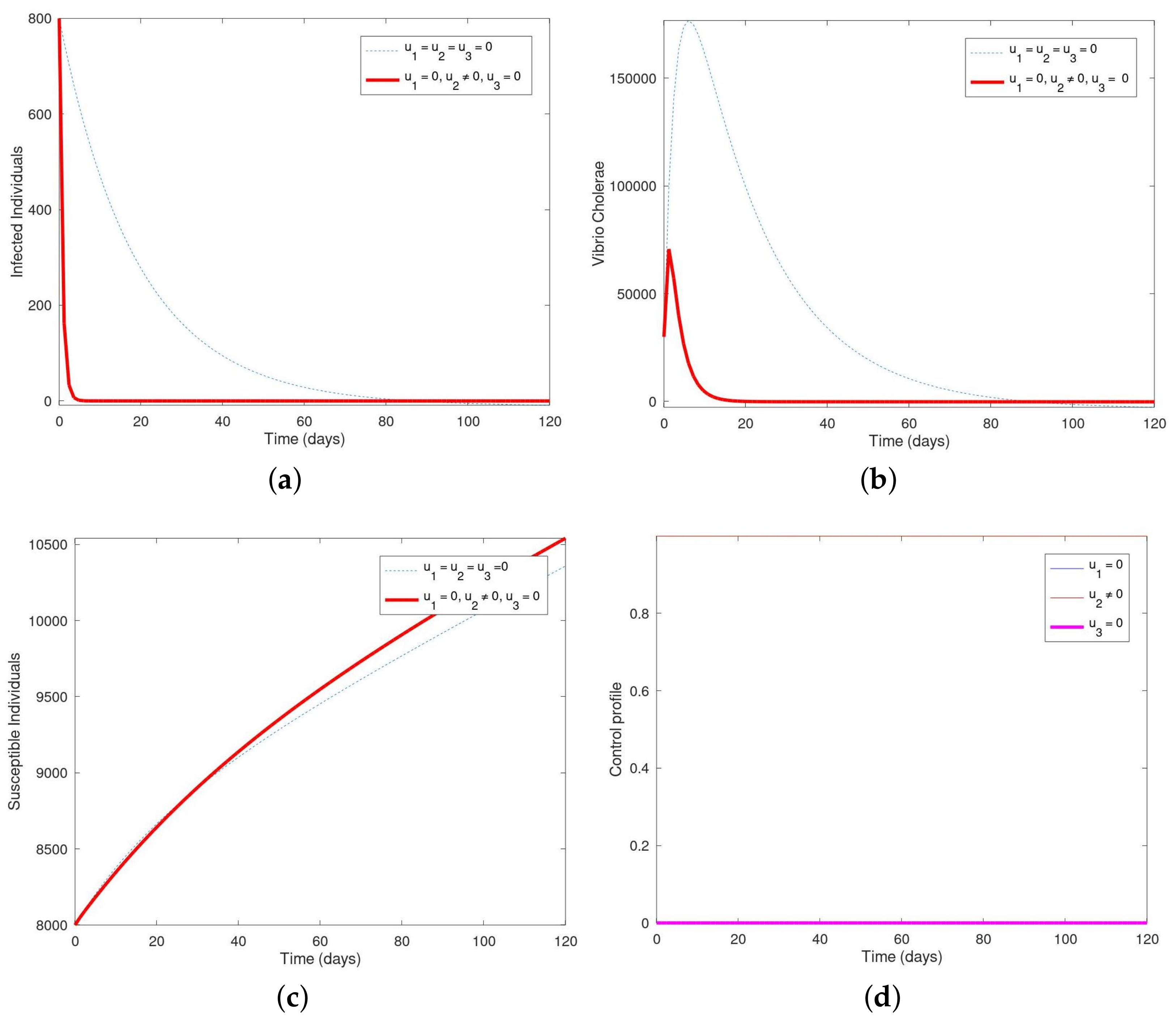
Here, we utilized only the control measure to optimize the objective functional J, while the control interventions and are kept at zero (i.e., were not utilized). In Figure 2, we present the plots of population of susceptible humans, infected humans, and vibrio cholerae and their control profile. In Figure 2a, the population of the infected human decreases sharply and by day 20, the disease is wiped out of the system in the presence of the control intervention. Figure 2b showed that the population of vibrio cholerae increases slightly and then dropped from day 20 until the end of 120 days in the presence of the intervention. It was observed in Figure 2c that the population of susceptible human with the control intervention were more than the susceptible human without the control. The control profile in Figure 2d showed that the control , remained constant from day 1 till the end of the 120 days while the others ( and ) maintained lower bounds.
6.3. Strategy C: Employing Sanitation, Hygiene, and Safe Water , Only
Here, we use only the control measure to optimize the objective functional J, while the control interventions and are kept at zero (i.e., were not utilized). In Figure 3a, it is observed that the population of vibrio cholerae increases slightly and then drops down completely after 80 days and the disease vanishes within 80–120 days. In Figure 3b the number of susceptible humans increases faster (with the control intervention) than without the control intervention. This implies that the control does not decrease the number of susceptible. In Figure 3c, the number of infected human population decreases completely in day 70 and vanishes by day 120. In Figure 3d, the control profile shows that the control , remained constant from day 1 till the end of the 120 days while the others ( and ) maintained lower bounds.
6.4. Strategy D: Employing the Control Interventions (, )
Here, we used control interventions () and () to optimize the objective functional J, while the control intervention () is kept at zero (i.e., were not utilized). In Figure 4a, the population of the infected human decreases drastically within the first 5 days and cholera was totally wiped out. In Figure 4b, the number of vibrio cholerae increases and then decreases until it vanishes. In Figure 4c, the number of susceptible humans completely decreases and vanishes from the system in the presence of the control intervention but increases without the control interventions. In Figure 4d, the control profile showed that the control () and () remained constant from day 1 till the end of the 120 days while () maintained lower bounds.
6.5. Strategy E: Employing the Control Interventions (, )
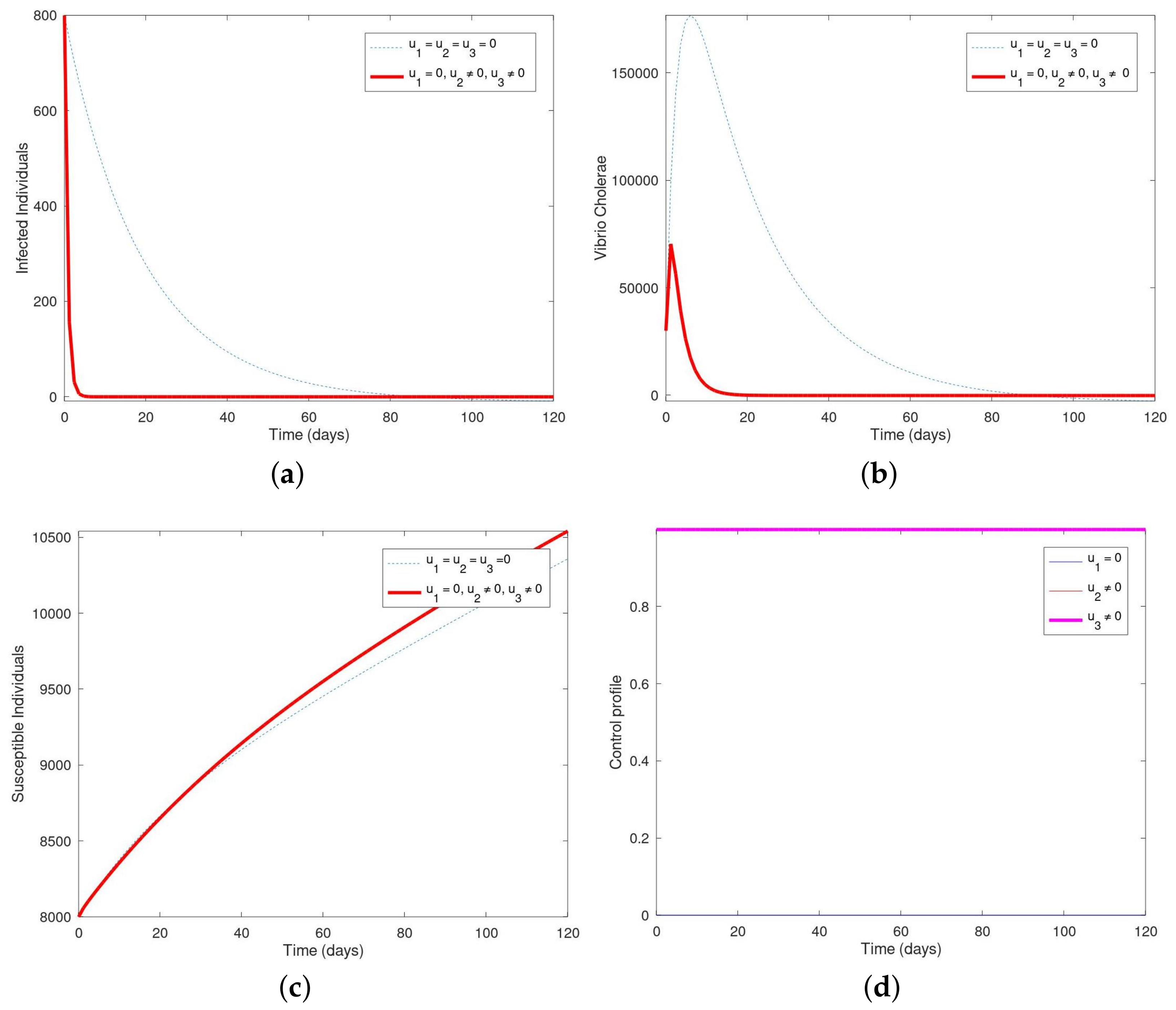
Here, we used control interventions () and () to optimize the objective functional J, while the control intervention () is kept at zero (i.e., were not utilized). In Figure 5a, the population of infected humans decreases essentially after 80 days until the disease was wiped out completely. Figure 5b reveals that the number of vibrio cholerae increases slightly and then decreases completely after 80 days and then vanishes completely. In Figure 5c, the number of susceptible humans completely decreases within 2 days and then vanishes from the system in the presence of the control interventions within 2–120 days. In Figure 5d, the control profile showed that the control (), and () remained constant from day 1 till the end of the 120 days while () maintained lower bounds.
6.6. Strategy F: Employing the Control Interventions (, )
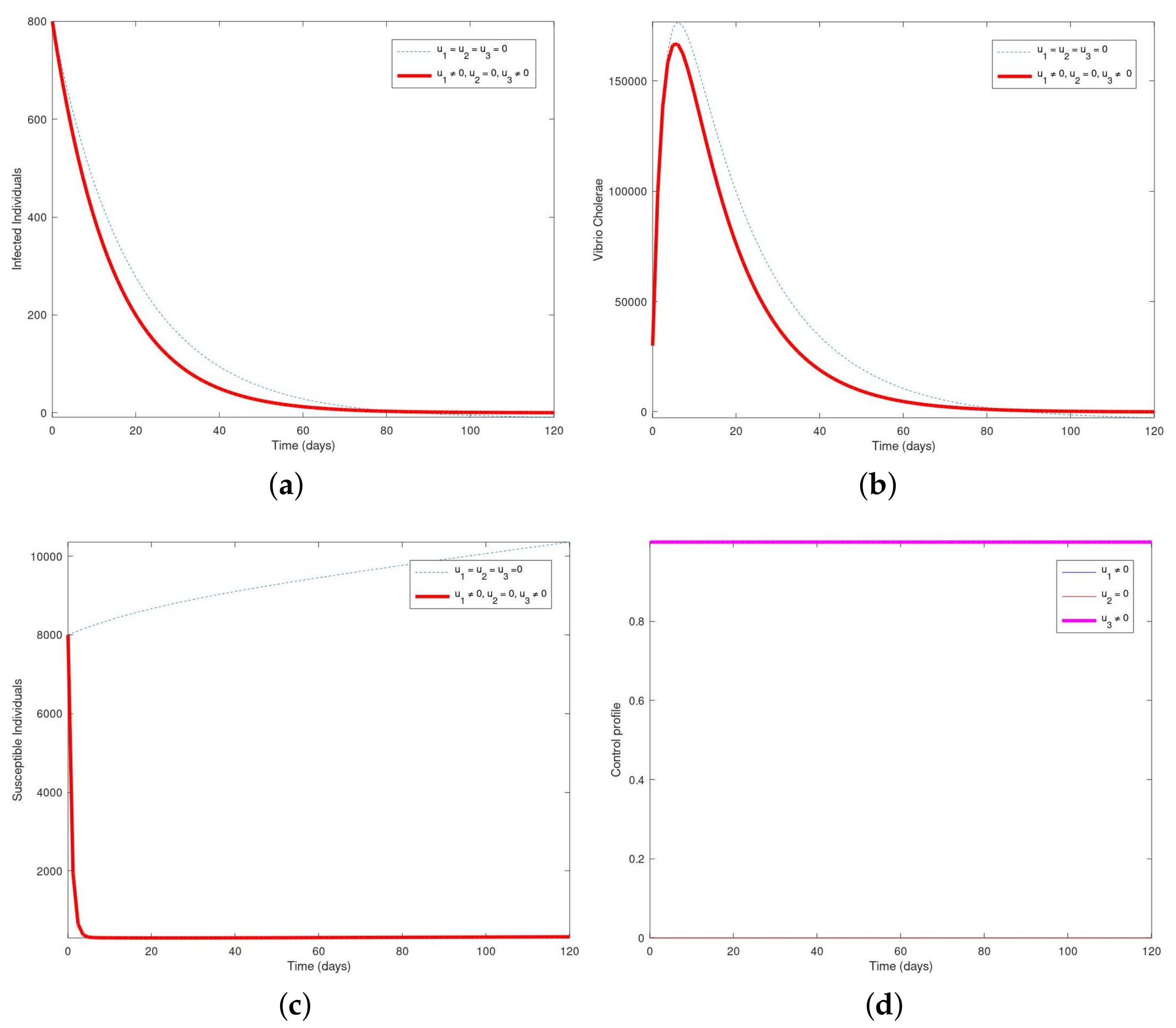
Here, we used control interventions () and () to optimize the objective functional J, while the control intervention () is kept at zero (i.e., were not utilized). In Figure 6a, the population of infected humans decreases within the first 2 days and then decreases until it vanishes completely from the system within 20–120 days. Figure 6b shows that the population of vibrio cholerae increases within the first 2 days and then decreases until it vanishes completely from the system within 20–120 days. In Figure 6c, the susceptible human population inctreases over the time period in the presence of the control intervention but was much slower within the control intervention. In Figure 6d, the control profile shows that the control (), and () remained constant from day 1 till the end of the 120 days while () maintained lower bounds.
6.7. Strategy G: Employing All the Three Control Interventions (, , )
Here, we used al the three control interventions (), (), and () to optimize the objective functional J. In Figure 7a, it was observed that the population of the infected human decreases within the first 2 days and then decreases until it vanishes completely from the system within 2–120 days in the presence of all the three interventions. In Figure 7b, the number of vibrio cholerae increases shortly within the first 20 days and then declines completely until it was wiped out from the system within 20–120 days. In Figure 7c, the number of susceptible humans begins decreasing within the first 2 days until it vanishes completely from the system. In Figure 7d, the control profile shows that the control (), (), and () remained stable from day 1 till the end of the 120 days.
7. Numerical Simulation of the SDE Model
In this section, we simulate our SDE model (5) by using the method of Milstein given the set of parameters in Table 4. We obtained results of stochastic model (5) for 200 runs, and presented and compared the mean of 200 runs of the stochastic model simulation with the results of the corresponding deterministic model as shown in Figure 8 and Figure 9, where the time series of all the variables of the model were plotted. It is observed from the figures that the mean of 200 runs of the stochastic simulation are very close to the simulation results of the deterministic model.
8. Conclusions
In this article, a nonlinear mathematical model to study the dynamics of the spread of cholera was developed and analyzed. The existence and global stability of the endemic equilibrium were discussed and it was shown that the endemic equilibrium is globally asymptotically stable whenever . Sensitivity and elasticity analysis of the model were also performed and it was revealed that some parameters had major and significant influence on the spread of cholera than others. The deterministic model was converted to stochastic model to capture some variabilities in the model and the results of the stochastic model were compared with their corresponding deterministic model. It was observed that the level of infected human population was the same with the simulation result of the corresponding deterministic model. It was observed from our work that optimal control applications revealed that the combinations of the interventions in the model had a great influence in the control of cholera. The numerical experiments revealed that optimal strategies to combat effectively the cholera was by the combinations of interventions in the model. The cholera model predicted the control of the disease by the combination of the three control interventions. The models developed predicted the decrease, control, and elimination of cholera morbidity and mortality through incorporating multiple control interventions into the model. Therefore, it is advised that the use of multiple control interventions be adopted for cholera in areas where there are sufficient resources. However, in areas where there are limited or lack of resources, it is advised that treatment of the symptomatic individuals with drug and/or administration of oral re-hydration solution (ORS) to the infected should be used. We therefore advise that in a situation where there are limited resources in the area, strategy B can be applied. The result of our study recommends that: (i) Hygiene promotion and social mobilization should be organized from time to time to reduce the transmission of cholera in the community and (ii) rhe fight against cholera can as well be successful by practising sanitation, hygiene, and drinking safe water. We recognize that this work will be a useful reference for any further study on monitoring the effect of multiple control strategies for cholera disease. We also believe that this study will help society at large to have an understanding of how the disease can be controlled through multiple control strategies in order to reduce the spread of the disease. Finally, the study will also help public health officers and environmental health workers organize seminars, training, and workshops to educate the community on the impact of multiple control strategies in reducing the spread of cholera disease. In future, we will like to study the influence of migration and environmental sanitation on the dynamics of transmission of cholera. The novelty in the work is that we introduced three time-dependent control interventions based on WHO recommendations into the model in order to predict the reduction/control of the cholera in the population as the obtained result may present a good framework for planning and decision making for any national control programs on cholera especially in communities with little or no resources. We plan to extend this work in the future by considering the impact of seasonality and climate variabilities. We also plan to study the influence of host heterogeneities on the transmission of cholera in the presence of multiple control interventions and it will also be interesting to look into the aspect of using real time data to parameterize the model developed.
Author Contributions
Conceptualization, E.A.B. and S.H.-M.; methodology, E.A.B. and S.H.-M.; software, E.A.B.; validation, E.A.B.; formal analysis, investigation, resources and data curation, E.A.B.; writing—original draft preparation, E.A.B. and S.H.-M.; writing—review and editing, E.A.B. and S.H.-M.; funding acquisition, S.H.-M. All authors have read and agreed to the published version of the manuscript.
Funding
This research received no external funding. The APC was funded by VAROPS granted by the Ministry of Defence of the Czech Republic.
Institutional Review Board Statement
Not applicable.
Informed Consent Statement
Not applicable.
Data Availability Statement
The data used to support the findings of this study are included within the article.
Acknowledgments
The author thanks the ICT Department of the Federal University Oye Ekiti, Ekiti State, Nigeria for the provision of space to complete this work and for their numerous support as well as the Ministry of Defence of the Czech Republic for the support via grant VAROPS.
Conflicts of Interest
The authors declare no conflict of interest.
References
- WHO. Cholera Country Profiles. Available online: http://www.who.int/cholera/countries/en/ (accessed on 13 January 2021).
- CDC. Cholera—Vibrio Cholera Infection. Available online: https://www.cdc.gov/cholera/ (accessed on 13 January 2021).
- Ngwa, M.C.; Liang, S.; Kracalik, I.T.; Morris, L.; Blackburn, J.K.; Mbam, L.M.; Ba Pouth, S.F.; Teboh, A.; Yang, Y.; Arabi, M.; et al. Cholera in Cameroon, 2000–2012: Spatial and Temporal Analysis at the Operational (Health District) and Sub Climate Levels. PLoS Negl. Trop. Dis. 2016, 10, e0005105. [Google Scholar] [CrossRef] [Green Version]
- Bakare, E.A.; Are, E.B.; Osanyinlusi, S. Impact of multiple control strategies on the Mathematical Modelling of Cholera transmission dynamics with asymptotic transmission. J. Niger. Assoc. Math. Phys. 2016, 36, 107–116. [Google Scholar]
- Ali, M.; Nelson, A.R.; Lopez, A.L.; Sack, D. Updated global burden of cholera in endemic countries. PLoS Negl. Trop. Dis. 2015, 9, e0003832. [Google Scholar] [CrossRef] [Green Version]
- Azman, A.S.; Rudolph, K.E.; Cummings, D.A.; Lessler, J. The incubation period of cholera: A systematic review. J Infect. 2013, 66, 432–438. [Google Scholar] [CrossRef] [Green Version]
- Faruque, S.M.; Naser, I.B.; Islam, M.J.; Faruque, A.S.; Ghosh, A.N.; Nair, G.B.; Sack, D.A.; Mekalanos, J.J. Seasonal epidemics of cholera inversely correlate with the prevalence of environmental cholrea phages. Proc. Natl. Acad. Sci. USA 2005, 102, 1702–1707. [Google Scholar] [CrossRef] [Green Version]
- Agarwal, M.; Verma, V. Modeling and analysis of the spread of an infectious disease cholera with environmental fluctuations. Appl. Appl. Math. 2012, 7, 406–425. [Google Scholar]
- Gil, A.I.; Louis, V.R.; Rivera, I.N.G.; Lipp, E.; Huq, A.; Lanata, C.F.; Taylor, D.N.; Russek-Cohen, E.; Choopun, N.; Sack, R.B.; et al. Occurrence and distribution of vibrio cholerae in the coastal environment of Peru. Environ. Microbiol. 2004, 6, 699–706. [Google Scholar] [CrossRef] [PubMed]
- Liao, S.; Wang, J. Stability analysis and application of a mathematical cholera model. Math. Biosci. Eng. 2011, 8, 733–752. [Google Scholar] [PubMed]
- Eisenberg, M.C.; Shuai, Z.; Tien, J.H.; van den Driessche, P. A cholera model in a patchy environment with water and human movement. Math. Biosci. 2013, 246, 105–112. [Google Scholar] [CrossRef] [PubMed]
- Louis, V.R.; Russek-Cohen, E.; Choopun, N.; Rivera, I.N.G.; Gangle, B.; Jiang, S.C.; Rubin, A.; Patz, J.E.; Huq, A.; Colwell, R.R. Predictability of vibrio cholerae in chesapeake bay. Appl. Environ. Microbiol. 2003, 69, 2773–2785. [Google Scholar] [CrossRef] [PubMed] [Green Version]
- Maheshwari, M.; Kiranmayi, K.N.B. Vibrio cholerae. Vet. World 2011, 4, 423–428. [Google Scholar] [CrossRef]
- Mondiale de la Santé, O.; World Health Organization. Cholera Vaccines: WHO Position Paper—August 2017 Weekly Epidemiological Record 25 August 2017. Wkly. Epidemiol. Rec. = Relevé épidéMiologique Hebdomadaire 2017, 92, 477–498. Available online: http://apps.who.int/iris/bitstream/10665/258764/1/WER9234-477-498.pdf (accessed on 13 January 2021).
- Dangbé, E.; Irépran, D.; Perasso, A.; Békollé, D. Mathematical modelling and numerical simulations of the influence of hygiene and seasons on the spread of cholera. Math. Biosci. 2018, 296, 60–70. [Google Scholar] [CrossRef] [PubMed]
- Mwasa, A.; Tchuenche, J.M. Mathematical analysis of a cholera model with public health interventions. Biosystems 2011, 105, 190–200. [Google Scholar] [CrossRef] [PubMed]
- Capasso, V. What IS First Name? A mathematical model for the 1973 cholera epidemic in the european mediterranean region. Rev. Epidemiol. Sante Publique 1979, 27, 121–132. [Google Scholar]
- Mosley, W.H.; Ahmed, S.; Benenson, A.S.; Ahmed, A. The relationship of vibiriocidal antibody titre to susceptibility to cholera in family contacts of cholera patients. Bull. World Health Organ. 1968, 38, 777–785. [Google Scholar]
- Shuai, Z.; Tien, J.H.; van den Driessche, P. Cholera models with hyperinfectivity and van den Driessche temporary immunity. Bull. Math. Biol. 2012, 74, 2423–2445. [Google Scholar] [CrossRef] [PubMed]
- Shuai, Z.; van den Driessche, P. Global dynamics of cholera models with differential infectivity. Math. Biosci. 2011, 234, 118–126. [Google Scholar] [CrossRef]
- Codeço, C.T. Endemic and epidemic dynamics of cholera: The role of the aquatic reservoir. BMC Infect. Dis. 2001, 1, 1–14. [Google Scholar] [CrossRef] [Green Version]
- Hartley, D.M.; Morris, J.G.; Smith, D.L. Hyperinfectivity: A critical element in the ability of V. cholerae to cause epidemics? PLoS Med. 2006, 3, 63–69. [Google Scholar] [CrossRef]
- Zhou, X.; Cui, J. Threshold dynamics for a cholera epidemic model with periodic transmission rate. Appl. Math. Model. 2013, 37, 3093–3101. [Google Scholar] [CrossRef]
- Tien, J.H.; Earn, D.J.D. Multiple transmission pathways and disease dynamics in a waterborne pathogen model. Bull. Math. Biol. 2010, 72, 1502. [Google Scholar] [CrossRef] [PubMed]
- Jensen, M.A.; Faruque, S.M.; Mekalanos, J.J.; Levin, B.R. Modeling the role of bacteriophage in the control of cholera outbreaks. Proc. Natl. Acad. Sci. USA 2006, 103, 4652–4657. [Google Scholar] [CrossRef] [Green Version]
- Mukandavire, Z.; Liao, S.; Wang, J.; Gaff, H.; Smith, D.L.; Morris, J.G. Estimating the reproductive numbers for the 2008–2009 cholera outbreaks in Zimbabwe. Proc. Natl. Acad. Sci. USA 2011, 108, 8767–8772. [Google Scholar] [CrossRef] [PubMed] [Green Version]
- Fung, I.C.H. Cholera transmission dynamic models for public health practitioners. Emerg. Themes Epidemiol. 2014, 11, 1. [Google Scholar] [CrossRef] [PubMed] [Green Version]
- Fister, K.R.; Gaff, H.; Lenhart, S.; Numfor, E.; Schaefer, E.; Wang, J. Optimal Control of Vaccination in an Age-Structured Cholera Model. Math. Stat. Model. Emerg. Re-Emerg. Infect. Dis. 2016, 221–248. [Google Scholar] [CrossRef]
- Kim, J.H.; Mogasale, V.; Burgess, C.; Wierzba, T.F. Impact of oral cholera vaccines in cholera-endemic countries: A mathematical modeling study. Vaccine 2016, 34, 2113–2120. [Google Scholar] [CrossRef] [PubMed] [Green Version]
- Sun, G.Q.; Xie, J.H.; Huang, S.H.; Jin, Z.; Li, M.T.; Liu, L. Transmission dynamics of cholera: Mathematical modeling and control strategies. Commun. Nonlinear Sci. Numer. Simul. 2017, 45, 235–244. [Google Scholar] [CrossRef]
- LaSalle, J.P. Stability theory of ordinary differential equations. J. Differ. Equs. 1968, 4, 57–65. [Google Scholar] [CrossRef] [Green Version]
- Yavuz, M.; Sene, N. Stability analysis and numerical computation of the fractional predator–prey model with the harvesting rate. Fractal Fract. 2020, 4, 35. [Google Scholar] [CrossRef]
- Parvaiz, A.N.; Mehmet, Y.; Sainat, Q.; Jian, Z.; Stuart, T. Modeling and analysis of COVID-19 epidemics with treatment in fractional derivatives using real data from Pakistan. Eur. Phys. J. Plus 2020, 135, 1–42. [Google Scholar]
- Parvaiz, A.N.; Kolade, M.O.; Mehmet, Y.; Jian, Z. Chaotic dynamics of a fractional order HIV-1 model involving AIDS-related cancer cells. Chaos Solitons Fractals 2020, 140, 110272. [Google Scholar]
- Mehmet, Y.; Necati, O. Analysis of an epidemic spreading model with exponential decay law. Math. Sci. Appl. E-Notes 2020, 8, 142–154. [Google Scholar]
- Hailemariam Hntsa, K.; Nerea Kahsay, B. Analysis of Cholera Epidemic Controlling Using Mathematical Modeling. Int. J. Math. Math. Sci. 2020, 2020, 7369204. [Google Scholar] [CrossRef]
- Shabami, I. Modelling the Effect of Screening on the Spread of HIV Infection in a Homogeneous Population with Infective Immigrants. Master’s Thesis, University of Der es Salaam, Dar es Salaam, Tanzania, 2010. [Google Scholar]
- Nakul, C.; Hyman, J.M.; Cushing, J.M. Determining important parameters in the spread of malaria through the sensitivity analysis of a mathematical model. Bull. Math. Biol. 2008, 70, 1272–1296. [Google Scholar]
- Zaman, G.; Kang, Y.H.; Jong, H.I. Stability analysis and optimal vaccination of an SIR epidemic model. BioSystems 2008, 93, 240–249. [Google Scholar] [CrossRef] [PubMed]
- Pontryagin, L.S.; Boltyanskii, V.G.; Gamkrelidze, R.V.; Mishchenko, E.F. The Mathematical Theory of Optimal Processes; Wiley: New York, NY, USA, 1962. [Google Scholar]
- Maturo, F. Unsupervised classification of ecological communities ranked according to their biodiversity patterns via a functional principal component decomposition of Hill’s numbers integral functions. Ecol. Indic. 2018, 90, 305–315. [Google Scholar] [CrossRef]
- Ferguson, J.; O’Leary, N.; Maturo, F.; Yusuf, S.; O’Donnell, M. Graphical comparisons of relative disease burden across multiple risk factors. BMC Med. Res. Methodol. 2019, 19, 186. [Google Scholar] [CrossRef] [PubMed] [Green Version]
- Urban, R.; Hoskova-Mayerova, S. Threat life cycle and its dynamics. Deturope 2017, 9, 93–109. [Google Scholar]
- Kudlak, A.; Urban, R.; Hoskova-Mayerova, S. Determination of the Financial Minimum in a Municipal Budget to Deal with Crisis Situations. Soft Comput. 2020, 24, 8607–8616. [Google Scholar] [CrossRef]
- Bekesiene, S.; Hoskova-Mayerova, S. Decision Tree—Based Classification Model for Identification of Effective Leadership Indicators in the Lithuania Army Forces. J. Math. Fund. Sci. 2018, 50, 121–141. [Google Scholar] [CrossRef]
- Tušer, I.; Hošková-Mayerová, Š. Emergency Management in Resolving an Emergency Situation. J. Risk Financ. Manag. 2020, 13, 262. [Google Scholar] [CrossRef]
Figure 1.
Simulation showing the population of (a) infected, (b) vibrio cholerae, (c) susceptible and (d) the control profile with only, where in Figure 1a, the infected human population decreases sharply over time. In Figure 1b, the population of vibrio cholerae increased within the first 20 days but dropped very sharply and wiped out completely until the end of 120 days. In Figure 1c, it was observed that the susceptible human population decreases with the control intervention in place but increases without the control. The control profile in Figure 1d shows that the control , remained stable from day 1 till the end of the 120 days while the others ( and ) maintained lower bounds.

Figure 2.
Simulation showing the population of (a) infected, (b) vibrio cholerae, (c) susceptible and (d) the control profile with , only. In Figure 2a, the population of the infected human decreases sharply and by day 20. Figure 2b showed that the population of vibrio cholerae increases slightly and then dropped from day 20 until the end of 120 days in the presence of the intervention. It was observed in Figure 2c that the population of susceptible human with the control intervention were more than the susceptible human without the control. The control profile in Figure 2d showed that the control , remained constant from day 1 till the end of the 120 days while the others ( and ) maintained lower bounds.

Figure 3.
Simulation showing the population of (a) infected, (b) vibrio cholerae, (c) susceptible and (d) the control profile with only. In Figure 3a, it is observed that the population of vibrio cholerae increases slightly and then drops down completely after 80 days and the disease vanishes within 80–120 days. In Figure 3b the number of susceptible humans increases faster (with the control intervention) than without the control intervention. This implies that the control does not decrease the number of susceptible. In Figure 3c, the number of infected human population decreases completely in day 70 and vanishes by day 120. In Figure 3d, the control profile shows that the control , remained constant from day 1 till the end of the 120 days while the others ( and ) maintained lower bounds.

Figure 4.
Simulation showing the population of (a) infected, (b) vibrio cholerae, (c) susceptible and (d) the control profile with . In Figure 4a, the population of the infected human decreases drastically within the first 5 days and cholera was totally wiped out. In Figure 4b, the number of vibrio cholerae increases and then decreases until it vanishes. In Figure 4c, the number of susceptible humans completely decreases and vanishes from the system in the presence of the control intervention but increases without the control interventions. In Figure 4d, the control profile showed that the control () and () remained constant from day 1 till the end of the 120 days while () maintained lower bounds.

Figure 5.
Simulation showing the population of (a) infected, (b) vibrio cholerae, (c) susceptible and (d) the control profile with . In Figure 5a, the population of infected humans decreases essentially after 80 days until the disease was wiped out completely. Figure 5b reveals that the number of vibrio cholerae increases slightly and then decreases completely after 80 days and then vanishes completely. In Figure 5c, the number of susceptible humans completely decreases within 2 days and then vanishes from the system in the presence of the control interventions within 2–120 days. In Figure 5d, the control profile showed that the control (), and () remained constant from day 1 till the end of the 120 days while () maintained lower bounds.

Figure 6.
Simulation showing the population of (a) infected, (b) vibrio cholerae, (c) susceptible and (d) the control profile with . In Figure 6a, the population of infected humans decreases within the first 2 days and then decreases until it vanishes completely from the system within 20–120 days. Figure 6b shows that the population of vibrio cholerae increases within the first 2 days and then decreases until it vanishes completely from the system within 20–120 days. In Figure 6c, the susceptible human population inctreases over the time period in the presence of the control intervention but was much slower within the control intervention. In Figure 6d, the control profile shows that the control (), and () remained constant from day 1 till the end of the 120 days while () maintained lower bounds.

Figure 7.
Simulation showing the population of (a) infected, (b) vibrio cholerae, (c) susceptible and (d) the control profile with . In Figure 7a, it was observed that the population of the infected human decreases within the first 2 days and then decreases until it vanishes completely from the system within 2–120 days in the presence of all the three interventions. In Figure 7b, the number of vibrio cholerae increases shortly within the first 20 days and then declines completely until it was wiped out from the system within 20–120 days. In Figure 7c, the number of susceptible humans begins decreasing within the first 2 days until it vanishes completely from the system. In Figure 7d, the control profile shows that the control (), (), and () remained stable from day 1 till the end of the 120 days.

Figure 8.
Simulation showing the dynamic behavior of susceptible humans, infected humans, recovered humans, and the Vibrio cholerae population and is given for ; ; . (a) revealed that the susceptible population decreases over time while the stochastic simulation are very close to the simulation results of the deterministic model. (b) also revealed that the vibrio cholerae population decreases over time while the population of the recovered human increases over time and their stochastic simulation are very close to the simulation results of the deterministic model.; ; ; ; ; ; ; ; ; ; ; ; ; ; ; and .

Figure 9.
Simulation showing the dynamic behavior of (a) susceptible humans, (b) infected humans, recovered humans, and the Vibrio cholerae population, and is given for ; ; ; ; ; ; ; ; ; ; ; ; ; ; ; ; ; and . We increased the recruitment rate of the susceptible population from 15 per day to 1 500 per day. Figure 9a, revealed that the susceptible population increases and then dropped slightly and the infected remained lowered and at steady state over time while the stochastic simulation is very close to the simulation results of the deterministic model but the fluctuation in the susceptible population became much stronger. Figure 9b, also revealed that the recovered population increases over time while the population of the vibrio cholerae decreases over time and their stochastic simulation are very close to the simulation results of the deterministic model.


Table 1.
Table showing the variables in the model.
| Variables | Description |
|---|---|
| S | Susceptible Human |
| I | Infected Human |
| R | Recovered Human |
| B | Vibrio Cholerae |
Table 2.
Descriptions of cholera control model parameters.
| Parameter | Symbol |
|---|---|
| Recruitment rate of susceptible population | A |
| Contribution of infected individuals to | |
| the population of Vibrio cholerae | |
| Natural death rate of human | |
| Net death rate of Vibrio cholerae | |
| Acquired temporary immunity | r |
| Disease-induced death rate | d |
| Concentration of Vibrio cholerae in water | K |
| Human spontaneous recovery rate | |
| Use of hygiene promotion and social mobilization | |
| Use of treatment by drug/oral re-hydration solution (ORS) | |
| Use of safe water, hygiene, and sanitation | |
| Rates of ingesting vibrios from the contaminated environment | |
| Rates of ingesting vibrios through human-to-human interaction | |
| loss of immunity |
Table 3.
Table showing numerical values of sensitivity indices for the cholera model.
| Parameter | Parameter Values | Sensitivity to |
|---|---|---|
| 100 | +0.24511 | |
| 0.2143 | +0.24511 | |
| 0.000002 | +0.755 | |
| A | 15 | +0.9999 |
| d | 0.015 | −0.2174 |
| 0.033 | −0.24511 | |
| 0.0000548 | −1.0000 | |
| 0.05 | −0.7245 | |
| r | 0.004 | −0.0579 |
| K | −0.24511 | |
| 0.025 | −0.24511 |
Table 4.
Table showing numerical values of parameters used in the simulations.
| Parameter | Symbol | Value | Source |
|---|---|---|---|
| Recruitment rate of susceptible population | A | 15/day | Assumed |
| Contribution of infected individuals to | |||
| the population of Vibrio cholerae | 100 cells/L-per day | [5] | |
| Natural death rate of human | 0.0000548/day | [18] | |
| Net death rate of Vibrio cholerae | 0.033/day | [5] | |
| Acquired temporary immunity | r | 0.004/day | [8,26] |
| Disease-induced death rate | d | 0.015/day | [26] |
| Concentration of Vibrio cholerae in water | K | cells/L | [26] |
| Human spontaneous recovery rate | 0.05 | [18] | |
| Use of oral cholera vaccine | 0.9 | Assumed | |
| Use of treatment by ORS | 0.91 | Assumed | |
| Personal hygiene/sanitation | 0.94 | Assumed | |
| Rates of ingesting vibrios from the CO * | 0.2143 | Assumed | |
| Eates of ingesting vibrios through H-H int. * | 0.000002 | Assumed | |
| Loss of immunity | 0.025 | Assumed |
* contaminated environment = CO; human-to-human interaction = H-H int.
Publisher’s Note: MDPI stays neutral with regard to jurisdictional claims in published maps and institutional affiliations. |
© 2021 by the authors. Licensee MDPI, Basel, Switzerland. This article is an open access article distributed under the terms and conditions of the Creative Commons Attribution (CC BY) license (https://creativecommons.org/licenses/by/4.0/).
Share and Cite
MDPI and ACS Style
Bakare, E.A.; Hoskova-Mayerova, S. Optimal Control Analysis of Cholera Dynamics in the Presence of Asymptotic Transmission. Axioms 2021, 10, 60. https://doi.org/10.3390/axioms10020060
AMA Style
Bakare EA, Hoskova-Mayerova S. Optimal Control Analysis of Cholera Dynamics in the Presence of Asymptotic Transmission. Axioms. 2021; 10(2):60. https://doi.org/10.3390/axioms10020060
Chicago/Turabian StyleBakare, Emmanuel A., and Sarka Hoskova-Mayerova. 2021. "Optimal Control Analysis of Cholera Dynamics in the Presence of Asymptotic Transmission" Axioms 10, no. 2: 60. https://doi.org/10.3390/axioms10020060
Note that from the first issue of 2016, this journal uses article numbers instead of page numbers. See further details here.