Decomposing the Krohn-Rhodes Form of Electroencephalography (EEG) Signals Using Jordan-Chevalley Decomposition Technique

Abstract

This paper explores how electroencephalography (EEG) signals in the Krohn-Rhodes form can be decomposed further using the Jordan-Chevalley decomposition technique. First, the recorded EEG signals of a seizure were transformed into a set of matrices. Each of these matrices was decomposed into its elementary components using the Krohn-Rhodes decomposition method. The components were then further decomposed into semisimple and nilpotent matrices using the Jordan-Chevalley decomposition. These matrices—which are the extended building blocks of elementary EEG signals—provide evidence that the EEG signals recorded during a seizure contain patterns similar to that of prime numbers.

1. Introduction and Motivation

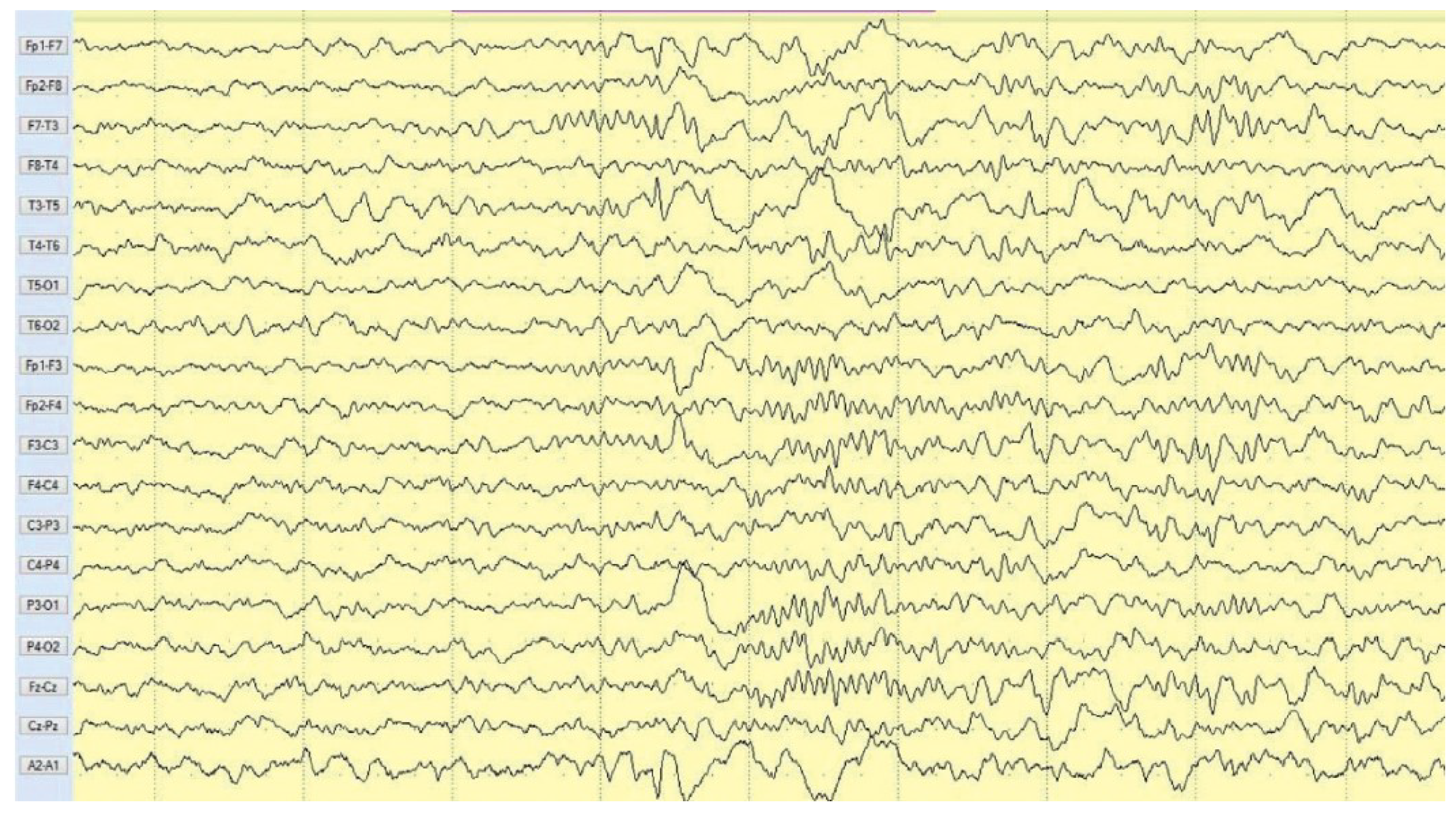
Epilepsy is a common neurological disease that, according to the World Health Organization, affects approximately $1\%$ of the world’s population [1]. The types of seizures experienced with epilepsy are divided into two groups: partial or focal onset seizures (in which the source of the seizure within the brain is localized) and generalized seizures (in which the source is distributed) [2]. Seizures are the product of a transitory and sudden electrical disturbance in the brain combined with exorbitant neuronal discharge, which is reflected in electroencephalography (EEG) signals. Recorded signals depict the electrical activity of the human brain; abnormal patterns—such as spikes, sharp waves, and wave complexes—can be observed (see Figure 1). However, EEG recording can be incomplete and inaccurate, as the system cannot distinguish between input objects and output objects.

EEG signals are often represented by vectors or matrices. This allows for the straightforward analysis and processing of data using widely understood methodologies like time-series analysis, spectral analysis, and matrix decomposition [3]. Among these, the Fourier Transform has emerged as a powerful tool that can characterize the frequency components of EEG signals and even establishing diagnostic importance. However, the Fourier transform also has some disadvantages. For one, it disregards the underlying nonlinear EEG dynamics that provide limited information about the electrical activity of the brain. Therefore, additional steps must be taken to extract the “hidden” information from EEG signals.

Fuzzy topographic topological mapping ($FTTM$) is a novel approach to solving the neuromagnetic inverse problems that determine epileptic foci [5]. Since its development, $FTTM$ has been utilized extensively to study the features of seizure patients’ recorded EEG signals (see References [6,7,8,9,10,11]). Most notably, Yun [12] claimed that one of the components of $FTTM$, known as magnetic contour ($MC$), obeys the associative law—which, in turn, is also satisfied by events in time [13]. The author concluded that $MC$ is a plane that contains information. This prompted Binjadhnan [14] to execute the Krohn-Rhodes decomposition on a set of square matrices of EEG signals during a seizure, $M{C}_n\left(\mathbb{R}\right)$. For convenience, the EEG signals during seizure are written as EEG signals for the rest of the paper unless stated otherwise. Remarkably, the results showed that the EEG signals that arose during an epileptic seizure do not occur randomly. Instead, they were ordered patterns with simple algebraic structures, namely periodic semigroups, affine scaling groups and the diagonal groups. One significant consequence of Krohn-Rhodes decomposition on EEG signals is Theorem 1.

Theorem 1

([14]). Any invertible square matrix of EEG signal readings at time t can be written as a product of elementary EEG signals in one and only one way.

Theorem 1 states that elementary EEG signals (unipotent and diagonal) are the building blocks of EEG signals. Binjadhnan [14] asserted that Theorem 1 was, in a sense, equivalent to the fundamental theorem of arithmetic, which stated that prime numbers were the multiplicative building blocks of positive integers. Furthermore, the EEG signals resemble some of the fundamental properties of prime numbers which can be summarized in

Table 1. Compatibility of EEG signals during a seizure to positive integers.

	EEG Signals	Positive Integers
Divisibility	Definition 1 ([14]). If $A\left(t\right)$ and $B\left(t\right)$ are EEG signals, we say that $A\left(t\right)$ divides $B\left(t\right)$, written as $A\left(t\right)\mid B\left(t\right)$, if there exist EEG signals $M\left(t\right)$ such that $B\left(t\right)=A\left(t\right)M\left(t\right)$, where $B\left(t\right)$ is an invertible EEG signals.	Definition 2 ([15]). If a and b are integers, we say that a divides b if there is an integer c such that $b=ac$.
Unique factorization theorem	(refer to Theorem 1)	Theorem 2 ([15]). Every positive integer greater than 1 can be written uniquely as a product of primes, with the prime factors in the product written in nondecreasing order.
Building blocks	Diagonal EEG signals group and the unipotent EEG signals group (direct sum of affine scaling groups plus identity group)	Prime numbers
Some properties	Theorem 3 ([14]). For EEG signals $A\left(t\right),B\left(t\right)$ and $C\left(t\right)$ the following hold: 1.  If $A\left(t\right)\mid B\left(t\right)$ and $B\left(t\right)\mid C\left(t\right)$, then $A\left(t\right)\mid C\left(t\right)$. 2.  If $A\left(t\right)\mid B\left(t\right)$ and $C\left(t\right)\mid B\left(t\right)$, then $\left(M\left(t\right)A\left(t\right)+N\left(t\right)C\left(t\right)\mid B\left(t\right)\right)$ for arbitrary EEG signals $M\left(t\right)$ and $N\left(t\right)$. 3.  Let $B\left(t\right)$ be a commutative EEG signals. If $A\left(t\right)\mid B\left(t\right)$ and $A\left(t\right)\mid C\left(t\right)$, then $A^2\left(t\right)\mid B\left(t\right)C\left(t\right)$. 4.  If $B\left(t\right)\mid C\left(t\right)$ and $A\left(t\right)\mid C\left(t\right)$, then $A\left(t\right)\mid B\left(t\right)$.	Theorem 4 ([15]). For prime number p and integers $a,b$ the following hold: 1.  If $p\mid ab$, then $p\mid a$ or $p\mid b$. 2.  If $p\mid a^2$, then $p\mid a$. 3.  If $p\mid a^n$, then $p\mid a$.

.

For centuries, mathematicians are baffled by the distribution of prime numbers within the positive integers. Hints can be found repeatedly in their distribution, indicating shadows of pattern, yet an accurate description of the actual pattern remains elusive. However, the recent development in the study of primes distribution revealed some intriguing results. Lemke Oliver and Soundararajan [16] discovered that prime numbers were not distributed randomly, but there are some patterns embedded in them. Marshall and Smith [17] take an unconventional approach by treating the prime numbers as a physical system and represented it as a differential equation that can predict the known results regarding the distribution of primes. Most recently, Torquato et al. [18,19,20] showed quasicrystals displayed scatter patterns that resembled the distribution of primes. Additionally, Bonanno and Mega [21], Iovane [22,23,24,25], and Garcia-Sandoval [26] demonstrated that the distribution of the primes follows a certain deterministic behavior. One significant result worthy to be mentioned is that the life cycles of different animal species are precisely prime numbers [27]. In general, prime numbers’ features are found in some properties of physical system.

Taking a similar approach of viewing the physical phenomena through the lens of prime numbers, Twin Prime Conjecture—one of the prominent conjectures in the study of prime numbers—provides a glimpse of extending the work of viewing elementary EEG signals as prime numbers.

Conjecture 1

(Twin Prime Conjecture [15]). There are infinitely many pairs of primes p and $p+2$.

The first few twin primes under 100 are $(3,5),(5,7),(11,13),(17,19),(29,31),(41,43),(59,61),$ and $(71,73)$. These primes—$5,7,13,19,31,43,61,73$ and so on—can be written as a sum of two primes, that is: $2+p$. Analogously, Barja [8] suggested the possibility of decomposing and writing the elementary EEG signals as a sum of its simpler components.

Any linear operator f over any field K can be written as a sum of two commuting operators—semisimple and nilpotent—through Jordan-Chevalley decomposition. The unique representation of f in terms of its commuting operators exists only when K is perfect due to the Jordan-Chevalley decomposition theorem [28]. Since the elementary EEG signals are linear operators over the field of real numbers $\mathbb{R}$, and the field $\mathbb{R}$ is a perfect (since it has characteristic 0); therefore it can be represented uniquely as a sum of its semisimple and nilpotent parts. In the present work, it is shown that elementary EEG signals can be decomposed via Jordan-Chevalley decomposition technique.

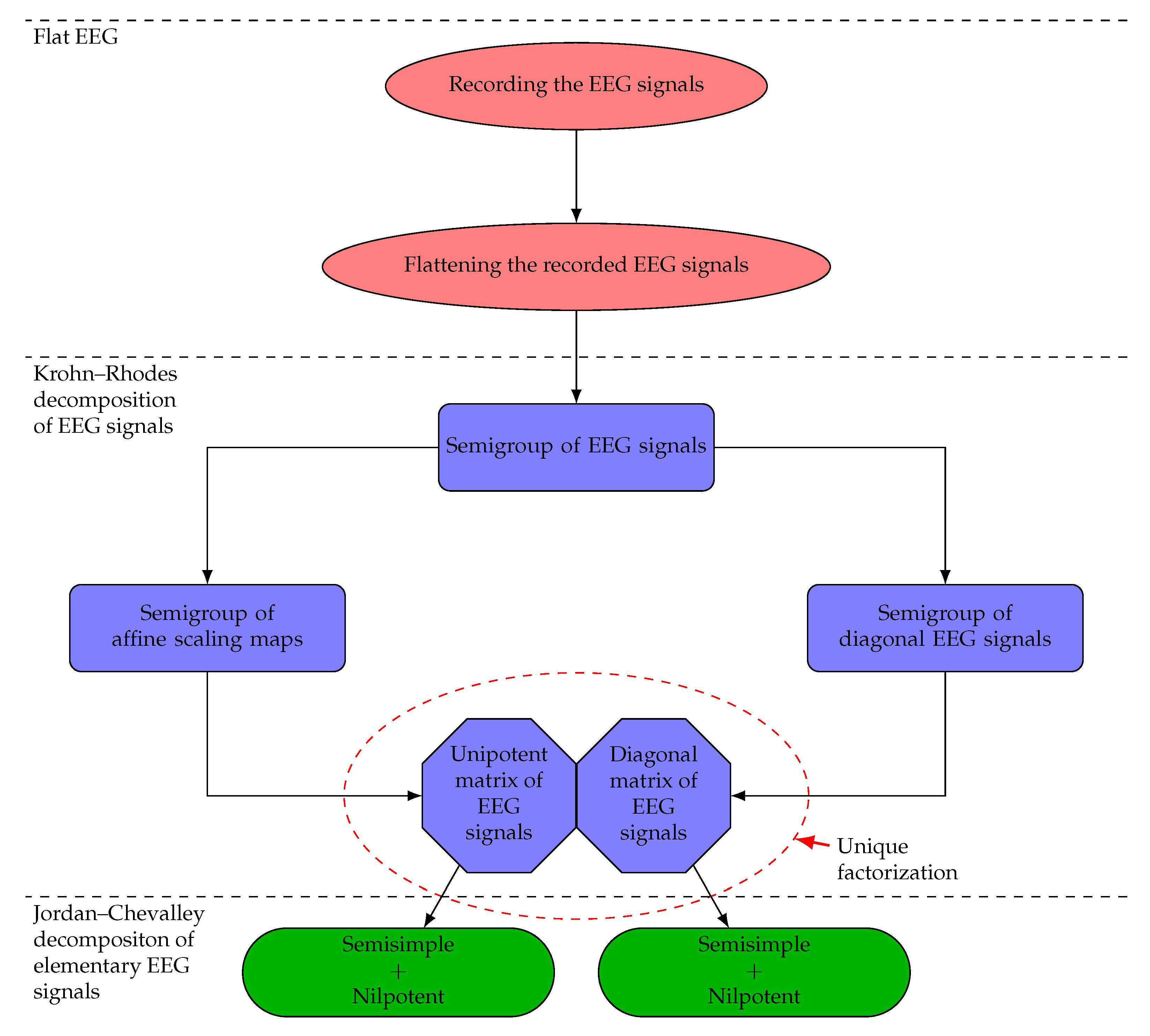
Beyond the introduction, this paper comprises five sections. In Section 2, the EEG signals recorded during an epileptic seizure are transformed into a set of upper triangular matrices and shown to be a semigroup under matrix multiplication. In Section 3, Krohn-Rhodes decomposition is applied to the semigroup to uncover the elementary components of the EEG signals. The results are discussed in Section 4, where the elementary EEG signals are further decomposed using the Jordan-Chevalley decomposition technique. The whole processes involved in decomposing the EEG signals into its summation of semisimple and nilpotent parts are summarized in Figure 2. Finally, we offer our concluding remarks and possible future studies.

2. Semigroup of EEG Signals during a Seizure

The EEG data of an epileptic seizure can be recorded as a set of $n\times n$ square matrices. Zakaria [29] first digitized EEG signals during an epileptic seizure at 256 samples per second using Nicolet One EEG software. Average potential difference (APD) was calculated from the samples every second, then stored in a file that contained the positioning of each electrode on a magnetic contour ($MC$) plane. The data were subsequently arranged as a set of square matrices.

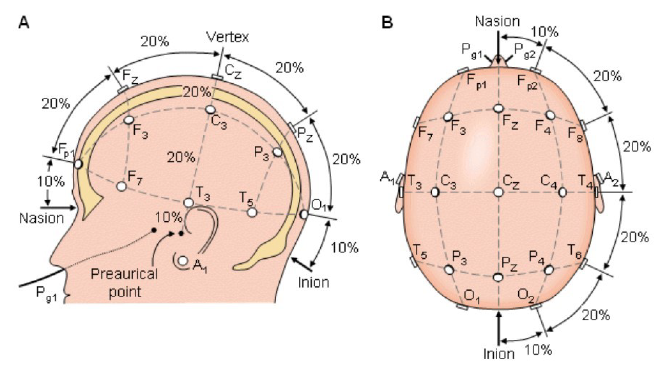
Differences in surface potential can be recorded using an array of electrodes on the scalp. The voltages among pairs of electrodes are computed, clarified, amplified, and recorded. The international Ten-Twenty System [30] is recommended for electrode placement, as it is considered the standard method for characterizing electrode locations at particular time intervals when recording scalp EEG [31]. The Ten-Twenty System depends on the connection between an electrode’s positioning and the underlying area of the cerebral cortex (“ten” and “twenty” refer to interelectrode distances of $10\%$ and $20\%$) [32]. The Ten-Twenty System is illustrated in Figure 3.

Figure 2A illustrates that almost all electrodes are positioned at a distance of $40\%$ or less from the vertex, $C_z$. Meanwhile, Figure 2B shows the electrode positions from the top of the head by modeling the head as a sphere. It is assumed that the hemisphere is at a distance of $80\%$ from the top of the head [29]. In other words, from the front of the head to the back is $F_{pz}$ to $O_z$, and from the left to the right is $T_3$ to $T_4$. Throughout the process, the APD at each second is stored in a file containing the positions of the electrodes on the $MC$ plane, as tabulated in

Table 2. Average potential difference (APD) at the sensor on a $MC$ [14].

Sensor	X	Y	APD
$F_{pz}$	$x_{21}$	$y_{21}$	$z_{21}$
$F_{p1}$	$x_{19}$	$y_{19}$	$z_{19}$
$F_{p2}$	$x_{20}$	$y_{20}$	$z_{20}$
$F_3$	$x_{15}$	$y_{15}$	$z_{15}$
$F_4$	$x_{16}$	$y_{16}$	$z_{16}$
$C_3$	$x_9$	$y_9$	$z_9$
$C_4$	$x_{10}$	$y_{10}$	$z_{10}$
$P_3$	$x_6$	$y_6$	$z_6$
$P_4$	$x_7$	$y_7$	$z_7$
$O_1$	$x_2$	$y_2$	$z_2$
$O_2$	$x_3$	$y_3$	$z_3$
$F_7$	$x_{17}$	$y_{17}$	$z_{17}$
$F_8$	$x_{18}$	$y_{18}$	$z_{18}$
$T_3$	$x_{11}$	$y_{11}$	$z_{11}$
$T_4$	$x_{12}$	$y_{12}$	$z_{12}$
$T_5$	$x_4$	$y_4$	$z_4$
$T_6$	$x_6$	$y_6$	$z_6$
$F_z$	$x_1$	$y_1$	$z_1$
$C_z$	$x_{13}$	$y_{13}$	$z_{13}$
$P_z$	$x_8$	$y_8$	$z_8$
$O_z$	$x_{14}$	$y_{14}$	$z_{14}$

.

The data in Table 2 can be written as a $5\times 5$ matrix, as shown below.

Let $x_1\le x_2\le \cdots \le x_{21},i,j=\left\{1,2,3,4,5\right\}$ and a function ${\beta }_{ij}$ is defined as follows:

$${\beta }_{ij}=\left\{\begin{array}{cc}\left(x_{(i-1)5+j},y_{(i-1)5+j}\right)\hfill & \mathrm{for}(i-1)5+j\le 21,\hfill \\ 0\hfill & \mathrm{for}(i-1)5+j>21.\hfill \end{array}\right.$$

The mapping ${\beta }_{ij}$ can be written as a matrix, as follows:

$$\left(\begin{array}{ccccc}{\beta }_{11}& {\beta }_{12}& {\beta }_{13}& {\beta }_{14}& {\beta }_{15}\\ {\beta }_{21}& {\beta }_{22}& {\beta }_{23}& {\beta }_{24}& {\beta }_{25}\\ {\beta }_{31}& {\beta }_{32}& {\beta }_{33}& {\beta }_{34}& {\beta }_{35}\\ {\beta }_{41}& {\beta }_{42}& {\beta }_{43}& {\beta }_{44}& {\beta }_{45}\\ {\beta }_{51}& {\beta }_{52}& {\beta }_{53}& {\beta }_{54}& {\beta }_{55}\end{array}\right).$$

Specifically,

$$\left(\begin{array}{ccccc}\left(x_1,y_1\right)& \left(x_2,y_2\right)& \left(x_3,y_3\right)& \left(x_4,y_4\right)& \left(x_5,y_5\right)\\ \left(x_6,y_6\right)& \left(x_7,y_7\right)& \left(x_8,y_8\right)& \left(x_9,y_9\right)& \left(x_{10},y_{10}\right)\\ \left(x_{11},y_{11}\right)& \left(x_{12},y_{12}\right)& \left(x_{13},y_{13}\right)& \left(x_{14},y_{14}\right)& \left(x_{15},y_{15}\right)\\ \left(x_{16},y_{16}\right)& \left(x_{17},y_{17}\right)& \left(x_{18},y_{18}\right)& \left(x_{19},y_{19}\right)& \left(x_{20},y_{20}\right)\\ \left(x_{21},y_{21}\right)& 0& 0& 0& 0\end{array}\right).$$

The corresponding square matrix is generated by substituting the analogy average potential difference of every element in the above matrix. Particularly, every single second of the APD is stored in a square matrix that contains the position of electrodes on the $MC$ plane. Therefore, $MC$ plane becomes a set of $n\times n$ matrices (EEG signals) as written in Equation (1):

$$M{C}_n\left(\mathbb{R}\right)=\left\{{\left[{\beta }_{ij}{\left(z\right)}_t\right]}_{n\times n}|i,j\in {\mathbb{Z}}^{+},{\beta }_{ij}{\left(z\right)}_t\in \mathbb{R}\right\},$$

(1)

where, ${\beta }_{ij}{\left(z\right)}_t$ is the potential difference reading of the EEG signals from a particular $ij$ sensor at time t.

As a sample of the transformed recorded EEG signals, two readings of EEG signals are presented in

Table 3. APD at the sensor on an $MC$ at $t=2$ of patient A [14].

Sensor	X	Y	APD
$F_{pz}$	$7.68$	0	0
$F_{p1}$	$7.3041$	$3.3733$	$33.94984375$
$F_{p2}$	$7.3041$	$-2.3733$	$15.32792969$
$F_3$	$3.3691$	$3.3691$	$22.99746094$
$F_4$	$3.3691$	$-3.3691$	$0.707890625$
$C_3$	0	$3.181$	$27.5621875$
$C_4$	0	$-3.1812$	$23.01671875$
$P_3$	$-3.3691$	$3.3691$	$84.15105469$
$P_4$	$-3.3691$	$-3.3691$	$25.2309375$
$O_1$	$-7.3041$	$2.3733$	$112.3017578$
$O_2$	$-7.3041$	$-2.3733$	$70.05695313$
$F_7$	$4.5142$	$6.2133$	$31.42472656$
$F_8$	$4.1542$	$-6.2133$	$15.34089844$
$T_3$	0	$7.68$	$58.33558594$
$T_4$	0	$-7.68$	$53.67203125$
$T_5$	$-4.5142$	$6.2133$	$114.2680859$
$T_6$	$-4.5142$	0	$102.3164453$
$F_z$	$3.1812$	0	$10.21890625$
$C_z$	0	0	$12.73027344$
$P_z$	$-3.1812$	0	$3.456171875$
$O_z$	$-7.68$	$y_{14}$	0

and

Table 4. APD at the sensor on an $MC$ at $t=3$ of patient A [14].

Sensor	X	Y	APD
$F_{pz}$	$7.68$	0	0
$F_{p1}$	$7.3041$	$3.3733$	$65.68265625$
$F_{p2}$	$7.3041$	$-2.3733$	$41.90457031$
$F_3$	$3.3691$	$3.3691$	$8.524765625$
$F_4$	$3.3691$	$-3.3691$	$0.0625$
$C_3$	0	$3.181$	$2.902265625$
$C_4$	0	$-3.1812$	$79.02796875$
$P_3$	$-3.3691$	$3.3691$	$110.2065234$
$P_4$	$-3.3691$	$-3.3691$	$63.74707031$
$O_1$	$-7.3041$	$2.3733$	$234.7169922$
$O_2$	$-7.3041$	$-2.3733$	$198.7374219$
$F_7$	$4.5142$	$6.2133$	$97.15632813$
$F_8$	$4.1542$	$-6.2133$	$76.86242188$
$T_3$	0	$7.68$	$138.7585156$
$T_4$	0	$-7.68$	$137.3880078$
$T_5$	$-4.5142$	$6.2133$	$209.6701172$
$T_6$	$-4.5142$	0	$230.6576563$
$F_z$	$3.1812$	0	$18.03042969$
$C_z$	0	0	$60.58832031$
$P_z$	$-3.1812$	0	$37.07589844$
$O_z$	$-7.68$	$y_{14}$	0

.

The data in Table 3 and Table 4 are reordered in the ascending order of the X values and tabulated in

Table 5. Reordering APD at the sensor at $t=2$ of patient A [14].

Sensor	X	Y	APD
$F_{pz}$	$-7.68$	0	0
$F_{p1}$	$-7.3041$	$2.3733$	$112.3017578$
$F_{p2}$	$-7.3041$	$-2.3733$	$70.05695313$
$F_3$	$-4.5142$	$6.2133$	$114.2680859$
$F_4$	$-4.5142$	$-6.2133$	$102.3164453$
$C_3$	$-3.3691$	$3.3691$	$84.15105469$
$C_4$	$-3.3691$	$-3.3691$	$25.2309375$
$P_3$	$-3.1812$	0	$3.456171875$
$P_4$	0	$3.1812$	$27.5621875$
$O_1$	0	$-3.1812$	$23.01671875$
$O_2$	0	$7.68$	$58.33558594$
$F_7$	0	$-7.68$	$53.67203125$
$F_8$	0	0	$12.73027344$
$T_3$	$3.1812$	0	$10.21890625$
$T_4$	$3.3691$	$3.3691$	$22.99746094$
$T_5$	$3.3691$	$-3.3691$	$0.707890625$
$T_6$	$4.5142$	$6.2133$	$31.42472656$
$F_z$	$4.5142$	$-6.2133$	$15.34089844$
$C_z$	$7.3041$	$2.3733$	$33.94984375$
$P_z$	$7.3041$	$-2.3733$	$15.32792969$
$O_z$	$7.68$	0	0

and

Table 6. Reordering APD at the sensor at $t=3$ of patient A [14].

Sensor	X	Y	APD
$F_{pz}$	$-7.68$	0	0
$F_{p1}$	$-7.3041$	$2.3733$	$234.7169922$
$F_{p2}$	$-7.3041$	$-2.3733$	$198.7374219$
$F_3$	$-4.5142$	$6.2133$	$209.6701172$
$F_4$	$-4.5142$	$-6.2133$	$230.6576563$
$C_3$	$-3.3691$	$3.3691$	$110.2065234$
$C_4$	$-3.3691$	$-3.3691$	$63.74707031$
$P_3$	$-3.1812$	0	$37.07589844$
$P_4$	0	$3.1812$	$2.902265625$
$O_1$	0	$-3.1812$	$79.02796875$
$O_2$	0	$7.68$	$138.7585156$
$F_7$	0	$-7.68$	$137.3880078$
$F_8$	0	0	$60.58832031$
$T_3$	$3.1812$	0	$18.03042969$
$T_4$	$3.3691$	$3.3691$	$8.524765625$
$T_5$	$3.3691$	$-3.3691$	$0.0625$
$T_6$	$4.5142$	$6.2133$	$97.15632813$
$F_z$	$4.5142$	$-6.2133$	$76.86242188$
$C_z$	$7.3041$	$2.3733$	$65.68265625$
$P_z$	$7.3041$	$-2.3733$	$41.90457031$
$O_z$	$7.68$	0	0

, respectively, through MATLAB programming that was developed by Binjadhnan [14]. They are then formed into $5\times 5$ square matrices.

$$A\left(2\right)=\left(\begin{array}{ccccc}0& 112.3018& 70.05695& 114.2681& 102.3164\\ 84.1511& 25.2309& 3.45617& 27.5622& 23.0167\\ 58.3356& 53.672& 12.7303& 10.2189& 22.9975\\ 0.707891& 31.4247& 15.3409& 33.9498& 15.3279\\ 0& 0& 0& 0& 0\end{array}\right).$$

$$A\left(3\right)=\left(\begin{array}{ccccc}0& 234.7169922& 198.7374219& 209.6701172& 230.6576563\\ 110.2065234& 63.74707031& 37.07589844& 2.902265625& 79.02796875\\ 138.7585156& 137.3880078& 60.58832031& 18.03042969& 8.524765625\\ 0.0625& 97.15632813& 76.86242188& 65.68265625& 41.90457031\\ 0& 0& 0& 0& 0\end{array}\right).$$

Binjadhnan and Ahmad [9] demonstrated that the nonempty set of square matrices of EEG signals, $M{C}_n\left(\mathbb{R}\right)$, is closed under matrix multiplication and thus satisfies the associative law. Consequently, the set $M{C}_n\left(\mathbb{R}\right)$ forms a semigroup with respect to matrix multiplication. This result indicates that the historical event is preserved in time [34]. In other words, $M{C}_n\left(\mathbb{R}\right)$ incorporates time as a property. Binjadhnan and Ahmad [9] also proved that $M{C}_n\left(\mathbb{R}\right)$ can be written as a set of $n\times n$ upper triangular matrices, $M{C}_n^{{}^{″}}\left(\mathbb{R}\right)$, and that this set also satisfies the axioms of a semigroup under matrix multiplication, per Theorem 5.

Theorem 5

([9]). The set of $n\times n$ upper triangular matrices $M{C}_n^{{}^{″}}\left(\mathbb{R}\right)$, is a semigroup under matrix multiplication.

Proof. 

i. Suppose that $A\left(t\right),B\left(t\right)\in M{C}_n^{{}^{″}}\left(\mathbb{R}\right)$ such that

$$A\left(t\right)=\left(\begin{array}{ccc}\beta 1_{1,1}& \cdots & \beta 1_{1,n}\\ ⋮& \ddots & ⋮\\ 0& \cdots & \beta 1_{n,n}\end{array}\right),B\left(t\right)=\left(\begin{array}{ccc}\beta 2_{1,1}& \cdots & \beta 2_{1,n}\\ ⋮& \ddots & ⋮\\ 0& \cdots & \beta 2_{n,n}\end{array}\right).$$

Then

$$\begin{array}{cc}\hfill A\left(t\right)B\left(t\right)=& \left(\begin{array}{ccc}\beta 1_{1,1}& \cdots & \beta 1_{1,n}\\ ⋮& \ddots & ⋮\\ 0& \cdots & \beta 1_{n,n}\end{array}\right)\left(\begin{array}{ccc}\beta 2_{1,1}& \cdots & \beta 2_{1,n}\\ ⋮& \ddots & ⋮\\ 0& \cdots & \beta 2_{n,n}\end{array}\right)\hfill \\ \hfill =& {\left(\sum _{j=1}^n\beta 1_{i,j}\beta 2_{ij}\right)}_{n,n}.\hfill \end{array}$$

Note that the entry in position $(i,k)$ is obtained by searching along the ith row of the first matrix and down the kth column of the second matrix.

$$\begin{array}{c}\left(\begin{array}{ccc}\beta 1_{1,1}& \cdots & \beta 1_{1,n}\\ ⋮& \ddots & ⋮\\ 0& \cdots & \beta 1_{n,n}\end{array}\right)\left(\begin{array}{ccc}\beta 2_{1,1}& \cdots & \beta 2_{1,n}\\ ⋮& \ddots & ⋮\\ 0& \cdots & \beta 2_{n,n}\end{array}\right)=\left(\begin{array}{ccc}{\displaystyle \sum _{j=1}^n\beta 1_{1,j}\beta 2_{j,1}}& \cdots & {\displaystyle \sum _{j=1}^n\beta 1_{1,j}\beta 2_{j,1}}\\ ⋮& \ddots & ⋮\\ 0& \cdots & {\displaystyle \sum _{j=1}^n\beta 1_{1,j}\beta 2_{j,1}}\end{array}\right).\end{array}$$

Now, $\beta 1_{i,j},\beta 2_{j,k}\in \mathbb{R}$ for a particular time $t\in {\mathbb{R}}^{+}$ and without loss of generality, $\beta 1_{i,j},\beta 2_{j,k}\in \mathbb{R}$ for some time $t\in {\mathbb{R}}^{+}$. Thus, ${\displaystyle \sum _{j=1}^n\beta 1_{i,j}\beta 2_{j,k}\in \mathbb{R}}$. Given that $A\left(t\right),B\left(t\right)\in M{C}_n^{{}^{″}}\left(\mathbb{R}\right)$ are arbitrary, it follows that $A\left(t\right)B\left(t\right)\in M{C}_n^{{}^{″}}\left(\mathbb{R}\right)$. Therefore, $M{C}_n^{{}^{″}}\left(\mathbb{R}\right)$ is closed with respect to matrix multiplication.

ii.  Suppose $A\left(t\right)={\left[\beta 1_{i,j}\right]}_{(n,n)},B\left(t\right)={\left[\beta 2_{j,k}\right]}_{(n,n)},C\left(t\right)={\left[\beta 3_{k,l}\right]}_{(n,n)}$. Then

$$A\left(t\right)B\left(t\right)={\left(\sum _{j=1}^n\beta 1_{i,j}\beta 2_{j,k}\right)}_{(n,n)},$$

 and

$$B\left(t\right)C\left(t\right)={\left(\sum _{j=1}^n\beta 2_{j,k}\beta 3_{k,l}\right)}_{(n,n)}.$$

Next,

$$\begin{array}{cc}\hfill \left(A\left(t\right)B\left(t\right)\right)C\left(t\right)& ={\left(\sum _{k=1}^n\left(\sum _{j=1}^n\beta 1_{i,j}\beta 2_{j,k}\right)\beta 3_{k,l}\right)}_{(n,n)}\hfill \\ \hfill & ={\left(\sum _{k=1}^n\sum _{j=1}^n\beta 1_{i,j}\beta 2_{j,k}\beta 3_{k,l}\right)}_{(n,n)},\hfill \end{array}$$

 and

$$\begin{array}{cc}\hfill A\left(t\right)\left(B\left(t\right)C\left(t\right)\right)& ={\left(\sum _{j=1}^n\beta 1_{i,j}\left(\sum _{k=1}^n\right)\beta 2_{j,k}\beta 3_{k,l}\right)}_{(n,n)}\hfill \\ \hfill & ={\left(\sum _{j=1}^n\sum _{k=1}^n\beta 1_{i,j}\beta 2_{j,k}\beta 3_{k,l}\right)}_{(n,n)}.\hfill \end{array}$$

Therefore, $\left(A\left(t\right)B\left(t\right)\right)=A\left(t\right)\left(B\left(t\right)C\left(t\right)\right)$. Consequently, the set $M{C}_n^{{}^{″}}\left(\mathbb{R}\right)$ is associative under matrix multiplication. Hence, (i) and (ii) imply that the set $M{C}_n^{{}^{″}}\left(\mathbb{R}\right)$ forms a semigroup under matrix multiplication.

□

3. Krohn-Rhodes Decomposition of ${\mathit{MC}}_{\mathit{n}}^{{}^{″}}\left(\mathbb{R}\right)$

In their ground-breaking work in the 1960s, Krohn and Rhodes proposed a method to express every finite semigroup as the divisor of a wreath product of finite groups and finite aperiodic semigroups [35,36]. Traditionally, the Krohn-Rhodes theory was applied only to finite semigroups; however, it has been generalized to well-behaved classes of infinite semigroups as well [37,38,39]. On this basis, Kambites and Steinberg [40] constructed a definitive wreath product decomposition for the semigroup of all $n\times n$ triangular matrices, $T_n\left(k\right)$, over a finite field k. However, the authors also obtained several results with applicability to a more general context in the process of developing the wreath product decomposition. Their proposed method is fully applicable in the case that the semigroup $T_n\left(k\right)$ is infinite. Binjadhnan, in [14], decomposed the infinite semigroup of EEG signals from an epileptic seizure over a field of real numbers by executing the decomposition technique developed by Kambites and Steinberg [40].

Before we explore the decomposition of $M{C}_n^{{}^{″}}\left(\mathbb{R}\right)$ using the Krohn-Rhodes method, some basic concepts of wreath product and affine transformation should be discussed. We have restricted this study to include only the special case of abstract monoids (as opposed to transformation semigroups, which are semigroups of transformations from a set to itself with identity function), as doing so is sufficient for our purposes.

Definition 3

([41]). If S and T are semigroups, then the Cartesian product $S\times T$ becomes a semigroup when $(s,t)(s^{\prime },t^{\prime })=(s^{\prime },t{t}^{\prime })$ This semigroup is considered a direct product of S and T.

Definition 4

([39]). Let S and T be monoids. The wreath product of S and T, denoted by $S\wr T$, is the monoid with the underlying set $S^T\times T$. Its multiplication is given by

$$(f,a)(g,b)=\left(g^a\circ f,ab\right),$$

where the multiplication of functions is pointwise. If $f\in S^T,t_1,t_2\in T$, then $f^{t_1}:T\to S$ is given by

$$f^{t_1}=f\left(t_2{t}_1\right).$$

The semigroup of EEG signals $M{C}_n\left(\mathbb{R}\right)$ was decomposed via Krohn-Rhodes decomposition with a field of real numbers $\mathbb{R}$ as the divisor of an alternating wreath product of groups and aperiodic monoids.

Theorem 6

([40]). Let $A,B$ and C be monoids. Then

1. 

$\left(A\wr B\right)\times C$ embeds in $A\wr (B\times C)$.

2. 

$\overline{A}\prec \tilde{X}\wr A$, where A is the monoid of the transformation of a set X.

3. 

$A\times B\prec A\wr B$.

Theorem 7 is the main inductive step for the decomposition of $M{C}_n^{{}^{″}}\left(\mathbb{R}\right)$. If $R\left(t\right)$ is a matrix, its transpose is written as $R^T\left(t\right)$.

Theorem 7

([14]). Let $n\ge 2$ and let $\mathbb{R}$ be a field of real numbers. Then

$$M{C}_n^{{}^{″}}\left(\mathbb{R}\right)\prec \left[ASM{C}_{n-1}\left(\mathbb{R}\right)\wr M{C}_{n-1}^{{}^{″}}\left(\mathbb{R}\right)\right]\times M{C}_1^{{}^{″}}\left(\mathbb{R}\right).w$$

Proof. 

Firstly, every element in $M{C}_n^{{}^{″}}\left(\mathbb{R}\right)$ is viewed as a block matrix

$$R\left(t\right)=\left(\begin{array}{cc}{Y}_{R\left(t\right)}& x_{R\left(t\right)}\\ 0& b_{R\left(t\right)}\end{array}\right),$$

where $Y_{R\left(t\right)}$ is an $(n-1)\times (n-1)$ matrix that lies within $M{C}_{n-1}^{{}^{″}}\left(\mathbb{R}\right),x_{R\left(t\right)}$ is an $n\times 1$ column vector and $b_{R\left(t\right)}$ is a $1\times 1$ matrix. Next, a mapping is defined as

$$\varphi :M{C}_n^{{}^{″}}\left(\mathbb{R}\right)\to \left[ASM{C}_{n-1}\left(\mathbb{R}\right)\wr M{C}_{n-1}^{{}^{″}}\left(\mathbb{R}\right)\right]\times M{C}_1^{{}^{″}}\left(\mathbb{R}\right),$$

such that

$$\varphi \left(R\left(t\right)\right)=\left(\left(f_{R\left(t\right)},Y_{R\left(t\right)}\right),b_{R\left(t\right)}\right),$$

where for all $Y_{R\left(t\right)}\in M{C}_{n-1}^{{}^{″}}\left(\mathbb{R}\right)$, and the element $f_{R\left(t\right)},Y_{R\left(t\right)}\in ASM{C}_{n-1}\mathbb{R}$ is given by

$$f_{R\left(t\right)},Y_{R\left(t\right)}\left(\overrightarrow{y}\right)=x_{R\left(t\right)}^T{Y}_{R\left(t\right)}^T+b_{R\left(t\right)}\overrightarrow{y}={\left(Y_{R\left(t\right)},x_{R\left(t\right)}+{\overrightarrow{y}}^T{b}_{R\left(t\right)}\right)}^T.$$

(2)

$\varphi$ is well-defined, since for any $R\left(t\right)\in M{C}_n^{{}^{″}}\left(\mathbb{R}\right)$, we have

$$\begin{array}{cc}\hfill {\left[f_{R\left(t\right)}I\left(t\right)\left(\overrightarrow{0}\right)\right]}^T& =I\left(t\right)x_{R\left(t\right)}+\overrightarrow{0}{b}_{R\left(t\right)}\hfill \\ \hfill & =x_{R\left(t\right)},\hfill \end{array}$$

where $I\left(t\right)\in M{C}_{n-1}^{{}^{″}}\left(\mathbb{R}\right)$ is the identity matrix and $\overrightarrow{0}\in {\mathbb{R}}^{n-1}$ is the zero vector. Furthermore, let $R\left(t_1\right),R\left(t_2\right)\in M{C}_n^{{}^{″}}\left(\mathbb{R}\right)$ and suppose that

$$\varphi \left(R\left(t_1\right)\right)=\left(\left(f_{R\left(t_1\right)},Y_{R\left(t_1\right)}\right),b_{R\left(t_1\right)}\right)=\left(\left(f_{R\left(t_2\right)},Y_{R\left(t_2\right)}\right),b_{R\left(t_2\right)}\right)=\varphi \left(R\left(t_2\right)\right).$$

Notice that $\left(f_{R\left(t_1\right)},Y_{R\left(t_1\right)}\right)=\left(f_{R\left(t_2\right)},Y_{R\left(t_2\right)}\right)$ means that $f_{R\left(t_1\right)}=f_{R\left(t_2\right)}$ (this equation implies that $x_{R\left(t_1\right)}=x_{R\left(t_2\right)}),Y_{R\left(t_1\right)}=Y_{R\left(t_2\right)}$ and $b_{R\left(t_1\right)}=b_{R\left(t_2\right)}$. Therefore, $R\left(t_1\right)=R\left(t_2\right)$. In other words, $\varphi$ is injective. Since $M{C}_n^{{}^{″}}\left(\mathbb{R}\right)$ is closed under matrix multiplication, it follows that for any $R\left(t_1\right),R\left(t_2\right)\in M{C}_n^{{}^{″}}\left(\mathbb{R}\right)$ as two block matrices, we have $R\left(t_1\right),R\left(t_2\right)\in M{C}_n^{{}^{″}}\left(\mathbb{R}\right)$ in terms of block matrix $\left(\begin{array}{cc}{Y}_{R\left(t\right)}& x_{R\left(t\right)}\\ 0& b_{R\left(t\right)}\end{array}\right)$. In other words, since

$$\left(\begin{array}{cc}{Y}_{R\left(t_1\right)}& x_{R\left(t_1\right)}\\ 0& b_{R\left(t_1\right)}\end{array}\right)\left(\begin{array}{cc}{Y}_{R\left(t_2\right)}& x_{R\left(t_2\right)}\\ 0& b_{R\left(t_2\right)}\end{array}\right)=\left(\begin{array}{cc}{Y}_{R\left(t_1\right)R\left(t_2\right)}& Y_{R\left(t_1\right)}{x}_{R\left(t_2\right)}+x_{R\left(t_1\right)}{b}_{R\left(t_2\right)}\\ 0& b_{R\left(t_1\right)}{b}_{R\left(t_2\right)}\end{array}\right),$$

we have

$$\begin{array}{cc}\hfill Y_{R\left(t_1\right)R\left(t_2\right)}& =Y_{R\left(t_1\right)}{Y}_{R\left(t_2\right)},b_{R\left(t_1\right)R\left(t_2\right)}\hfill \\ \hfill & =b_{R\left(t_1\right)}{b}_{R\left(t_2\right)},\hfill \end{array}$$

and

$$x_{R\left(t_1\right)R\left(t_2\right)}=Y_{R\left(t_1\right)}{x}_{R\left(t_2\right)}+x_{R\left(t_1\right)}{b}_{R\left(t_2\right)}.$$

Next, we have to show that

$$\varphi \left(R\left(t_1\right),R\left(t_2\right)\right)=\varphi \left(R\left(t_1\right)\right)\varphi \left(R\left(t_2\right)\right),$$

for all choices of $R\left(t_1\right),R\left(t_2\right)\in M{C}_n^{{}^{″}}\left(\mathbb{R}\right)$. Suppose $R\left(t_1\right),R\left(t_2\right)\in M{C}_n^{{}^{″}}\left(\mathbb{R}\right)$. Then

$$\varphi \left(R\left(t_1\right)R\left(t_2\right)\right)=\left(\left(f_{R\left(t_1\right)R\left(t_2\right)},Y_{R\left(t_1\right)R\left(t_2\right)}\right),b_{R\left(t_1\right)R\left(t_2\right)}\right).$$

(3)

On the other hand,

$$\begin{array}{cc}\varphi \left(R\left(t_1\right)\right)\varphi \left(R\left(t_2\right)\right)\hfill & =\left(\left(F_{R\left(t_1\right)},Y_{R\left(t_1\right)}\right),b_{R\left(t_1\right)})\right)\left(\left(f_{R\left(t_2\right)},Y_{R\left(t_2\right)}\right),b_{R\left(t_2\right)}\right)\hfill \\ \hfill & =\left(\left(f_{R\left(t_1\right)},Y_{R\left(t_2\right)}\right)\left(f_{R\left(t_2\right)},Y_{R\left(t_2\right)}\right),b_{R\left(t_1\right)}{b}_{R\left(t_2\right)}\right)—\mathrm{by}\mathrm{Definition}3\hfill \\ \hfill & =\left(\left(f_{R\left(t_2\right)}^{Y_{R\left(t_1\right)}}\circ f_{R\left(t_1\right)},Y_{R\left(t_1\right)}{Y}_{R\left(t_2\right)}\right),b_{R\left(t_1\right)}{b}_{R\left(t_2\right)}\right)—\mathrm{by}\mathrm{Definition}4\hfill \\ \hfill & =\left(\left(f_{R\left(t_2\right)}^{Y_{R\left(t_1\right)}}\circ f_{R\left(t_1\right)},Y_{R\left(t_1\right)R\left(t_2\right)}\right),b_{R\left(t_1\right)}{b}_{R\left(t_2\right)}\right).\hfill \end{array}$$

(4)

To complete the proof, we must show that $f_{R\left(t_1\right)R\left(t_2\right)}=f_{R\left(t_2\right)}^{Y_{R\left(t_1\right)}}\circ f_{R\left(t_1\right)}$. We need to show that $f_{R\left(t_1\right)R\left(t_2\right)}X\left(\overrightarrow{y}\right)=\left(f_{R\left(t_2\right)}X{Y}_{R\left(t_1\right)}\circ f_{R\left(t_1\right)}X\right)\left(\overrightarrow{y}\right)$ for all $\overrightarrow{y}\in {\mathbb{R}}^{+}$ and $X\in M{C}_{n-1}^{{}^{″}}\left(\mathbb{R}\right)$.

$$\begin{array}{cc}{f}_{R\left(t_1\right)R\left(t_2\right)X\left(\overrightarrow{y}\right)}\hfill & =\left(X_{X_{R\left(t_1\right)R\left(t_2\right)}}+{\overrightarrow{y}}^T{b}_{R\left(t_1\right)}{b}_{R\left(t_2\right)}\right)—\mathrm{by}\mathrm{Equation}(2)\hfill \\ \hfill & ={\left(X\left(Y_{R\left(t_1\right)R\left(t_2\right)}+x_{R\left(t_1\right)}{b}_{R\left(t_2\right)}\right)+{\overrightarrow{y}}^T{b}_{R\left(t_1\right)}{b}_R\left(t_2\right)\right)}^T\hfill \\ \hfill & ={\left(X{Y}_{R\left(t_1\right)}{x}_{R\left(t_2\right)}+X{x}_{R\left(t_1\right)}{b}_{R\left(t_2\right)}+{\overrightarrow{y}}^T{b}_{R\left(t_1\right)}{b}_{R\left(t_2\right)}\right)}^T\hfill \\ \hfill & ={\left(X{Y}_{R\left(t_1\right)}{x}_{R\left(t_2\right)}+\left(X{x}_{R\left(t_1\right)}+{\overrightarrow{y}}^T{b}_{R\left(t_1\right)}\right)b_{R\left(t_2\right)}\right)}^T\hfill \\ \hfill & ={\left(X{Y}_{R\left(t_1\right)}{x}_R\left(t_2\right)\right)}^T+{\left(X{x}_{R\left(t_1\right)}+{\overrightarrow{y}}^T{b}_R\left(t_1\right)\right)}^T{b}_{R\left(t_2\right)}-(\mathrm{since}{(A+B)}^T=A^T+B^T)\hfill \\ \hfill & ={\left(X{Y}_{R\left(t_1\right)}{x}_{R\left(t_2\right)}\right)}^T+\left(f_{R\left(t_1\right)}X\left(\overrightarrow{y}\right)\right)b_{R\left(t_2\right)}—\mathrm{by}\mathrm{Equation}(2)\hfill \\ \hfill & ={\left(X{Y}_{R\left(t_1\right)}{x}_{R\left(t_2\right)}+\left(\left(f_{R\left(t_1\right)}X{\left(\overrightarrow{y}\right)}^T{b}_{R\left(t_2\right)}\right)\right)\right)}^T\hfill \\ \hfill & =f_{R\left(t_2\right)}X{Y}_{R\left(t_1\right)}\left(f_{R\left(t_1\right)}X\left(\overrightarrow{y}\right)\right)—\mathrm{by}\mathrm{Equation}(2)\hfill \\ \hfill & =\left(f_{R\left(t_2\right)}X{Y}_{R\left(t_1\right)}\circ f_{R\left(t_1\right)}X\right)(\overrightarrow{y}).\hfill \end{array}$$

(5)

From Equations (3)–(5), we have

$$\varphi \left(R\left(t_1\right),R\left(t_2\right)\right)=\varphi \left(R\left(t_1\right)\right)\varphi \left(R\left(t_2\right)\right).$$

Therefore, $M{C}_n^{{}^{″}}\left(\mathbb{R}\right)\prec \left[ASM{C}_{n-1}\left(\mathbb{R}\right)\wr M{C}_{n-1}^{{}^{″}}\left(\mathbb{R}\right)\right]\times M{C}_1^{{}^{″}}\left(\mathbb{R}\right)$. □

Theorem 8.

Let $n\ge 2$ and $\mathbb{R}$ be a field of real numbers. Then

$$M{C}_n^{{}^{″}}\left(\mathbb{R}\right)\prec ASM{C}_{n-1}\left(\mathbb{R}\right)\wr ASM{C}_{n-2}\left(\mathbb{R}\right)\wr \cdots \wr \left(ASM{C}_1\left(\mathbb{R}\right)\times M{C}_1^{{}^{″}}{\left(\mathbb{R}\right)}^n\right).$$

Proof. 

We use induction on n. When $n=2$, the following is obtained by Theorems 6 and 7:

$$M{C}_2^{{}^{″}}\left(\mathbb{R}\right)\prec \left[ASM{C}_1\left(\mathbb{R}\right)\wr M{C}_1^{{}^{″}}\left(\mathbb{R}\right)\right]\times M{C}_1^{{}^{″}}\left(\mathbb{R}\right)\prec ASM{C}_1\left(\mathbb{R}\right)\wr M{C}_1^{{}^{″}}{\left(\mathbb{R}\right)}^2.$$

Next, let $n\ge 3$. It is assumed to be true for $n=k-1$. Therefore, for $n=k$

$$\begin{array}{cc}M{C}_k^{{}^{″}}\left(\mathbb{R}\right)\hfill & \prec \left[ASM{C}_{k-1}\left(\mathbb{R}\right)\wr M{C}_{k-1}^{{}^{″}}\left(\mathbb{R}\right)\right]\times M{C}_1^{{}^{″}}\left(\mathbb{R}\right)\hfill \\ \hfill & \prec \left[ASM{C}_{k-1}\left(\mathbb{R}\right)\wr \left[ASM{C}_{k-2}\left(\mathbb{R}\right)\wr ASM{C}_{k-2}\left(\mathbb{R}\right)\wr \cdots \wr ASM{C}_1\left(\mathbb{R}\right)\times M{C}_1^{{}^{″}}{\left(\mathbb{R}\right)}^{-1}\right]\right]\times M{C}_1^{{}^{″}}\left(\mathbb{R}\right)\hfill \\ \hfill & \prec ASM{C}_{k-1}\left(\mathbb{R}\right)\wr ASM{C}_{k-2}\left(\mathbb{R}\right)\wr \cdots \wr \left(ASM{C}_1\left(\mathbb{R}\right)\times M{C}_1^{{}^{″}}{\left(\mathbb{R}\right)}^k\right)—\left(\mathrm{by}\mathrm{Theorem}6\right).\hfill \end{array}$$

□

The decomposition of the semigroup of EEG signals during an epileptic seizure—in terms of affine scaling groups, diagonal groups, and aperiodic semigroups—is summarized in the following steps.

Step 1:

Use Nicolet One EEG software to get a Fast Fourier Transform (FFT) of raw data from the signals (i.e., the potential difference).

Step 2:

Use the Flat EEG method to store the APD at each second in a file that contains the positions of the electrodes on the $MC$ plane.

Step 3:

Rewrite the APD at the sensor on $MC$ in terms of a square matrix in $M{C}_n$.

Step 4:

Apply Schur decomposition to the output from Step 3, generating a set of upper triangular matrices that represents the semigroup $M{C}_n^{*}\left(\mathbb{R}\right)$ under matrix multiplication.

Step 5:

View each element in $M{C}_n^{*}\left(\mathbb{R}\right)$ as a block matrix

$$R\left(t\right)=\left(\begin{array}{cc}{Y}_{R\left(t\right)}& x_{R\left(t\right)}\\ 0& b_{R\left(t\right)}\end{array}\right),$$

where $Y_{R\left(t\right)}$ is an $(n-1)\times (n-1)$ matrix that lies in $M{C}_{n-1}^{"},x_{R\left(t\right)}$ an $n\times 1$ column vector and $b_{R\left(t\right)}$ is a $1\times 1$ matrix.

Step 6:

Use Theorem 7 to get the image of $R\left(t\right)$ as Equation (6)

$$\varphi \left(R\left(t\right)\right)=\left((f_{R\left(t\right)},Y_{R\left(t\right)}),b_{R\left(t\right)}\right),$$

(6)

where for every $Y_{R\left(t\right)}\in M{C}_{n-1}^{"}\left(\mathbb{R}\right)$, the element $f_{R\left(t\right)}{Y}_{R\left(t\right)}\in ASM{C}_{n-1}\left(\mathbb{R}\right)$ is given by

$$\begin{array}{cc}\hfill f_{R\left(t\right)}{Y}_{R\left(t\right)}\left(\overrightarrow{y}\right)=& x_{R\left(t\right)}^T{Y}_{R\left(t\right)}^T+b_{R\left(t\right)}\overrightarrow{y}\hfill \\ \hfill =& {\left(Y_{R\left(t\right)}{x}_{R\left(t\right)}+{\overrightarrow{y}}^T{b}_{R\left(t\right)}\right)}^T.\hfill \end{array}$$

Step 7:

Repeat Steps 5 and 6 on a new upper triangular matrix $Y_{R\left(t\right)}$.

In Section 2, Steps 1 through 3 were conducted in order to transform the recorded EEG signals into a set of square matrices. Now, the square matrices can be decomposed into upper triangular matrices. For every square matrix $A\left(t\right)$ at any time t, a $5\times 5$ orthogonal matrix $Q\left(t\right)$ and upper triangular matrix $R\left(t\right)$ is found using Schur decomposition, as per Equation (7).

$$Q^T\left(t\right)A\left(t\right)Q\left(t\right)=R\left(t\right)=\left(\begin{array}{cccc}{R}_{11}& R_{12}& \cdots & R_{1k}\\ 0& R_{22}& \cdots & R_{2k}\\ ⋮& ⋮& \ddots & ⋮\\ 0& 0& \cdots & R_{kk}\end{array}\right).$$

(7)

For example, matrices $Q\left(2\right)$ and $R\left(2\right)$ are obtained when Schur decomposition is executed on matrix $A\left(2\right)$.

$$\begin{array}{cc}\hfill Q\left(2\right)=& \left(\begin{array}{ccccc}0.70047& 0.6207& 0.28411& -0.20821& 0\\ 0.49558& -0.74501& 0.44828& 0.071377& 0\\ 0.47767& -0.20406& -0.84136& -0.14938& 0\\ 0.18862& 0.15727& -0.10331& 0.96397& 0\\ 0& 0& 0& 0& 1\end{array}\right),\hfill \\ \hfill R\left(2\right)=& \left(\begin{array}{ccccc}157.9953& -43.30315& 13.81193& 86.52425& 96.95254\\ 0& -79.1872& -40.6489& 64.3903& 44.1821\\ 0& 0& -16.6237& 32.214& 18.4712\\ 0& 0& 0& 9.7267& -8.3196\\ 0& 0& 0& 0& 0\end{array}\right).\hfill \end{array}$$

Matrix $R\left(2\right)$ can be viewed as a block matrix

$${\left(\begin{array}{cc}{Y}_{R\left(2\right)}& x_{R\left(2\right)}\\ 0& b_{R\left(2\right)}\end{array}\right)}_{5\times 5},$$

and $x_{R\left(2\right)}^T{Y}_{R\left(2\right)}^T$ for $R\left(2\right)$ and the constant map $f_{4R\left(2\right)}{Y}_{4\times 4R\left(2\right)}\left({\overrightarrow{y}}_{1\times 4}\right)$ for every ${\overrightarrow{y}}_{1\times 4}$ are obtained. $x_{Y_{R\left(2\right)}}^T{Y}_{Y_{R\left(2\right)}}^T$ for $Y_{4\times 4R\left(2\right)},x_{Y_{Y_{R\left(2\right)}}}^T{Y}_{Y_{Y_{R\left(2\right)}}}^T$ for $Y_{Y_{3\times 3R\left(2\right)}}$ and $x_{Y_{Y_{Y_{R\left(2\right)}}}}^T{Y}_{Y_{Y_{Y_{R\left(2\right)}}}}^T$ for $Y_{Y_{Y_{2\times 2R\left(2\right)}}}$ are also obtained.

Next, the affine scaling transformations $f_{iR\left(2\right)}\left({\overrightarrow{y}}_{1\times i}\right)$ is developed for chosen vectors ${\overrightarrow{y}}_{1\times i}(1\le i\le 3)$. In addition, the direct sum of the affine scaling maps is determined. Finally, the identity matrix is added to the direct sum of the affine scaling maps to determine the elementary unipotent matrix $U\left(2\right)$. Then, the direct product of $U\left(2\right)$ and the elementary diagonal matrix $D\left(2\right)$ is determined, and it is isomorphic to $Y_{R\left(t\right)}$.

The correspondent matrices and numerical computations described above for $R\left(2\right)$ are summarized as follows:

$$\begin{array}{cc}\hfill Y_{R\left(2\right)}=& \left(\begin{array}{cccc}157.9953& -43.30315& 13.81193& 86.52425\\ 0& -79.1872& -40.6489& 64.3903\\ 0& 0& -16.6237& 32.214\\ 0& 0& 0& 9.7267\end{array}\right),\hfill \\ \hfill x_{R\left(2\right)}=& \left(\begin{array}{c}96.95254\\ 44.1821\\ 18.4712\\ -8.3196\end{array}\right),\hfill \\ \hfill b_{R\left(2\right)}=& 0,\hfill \\ \hfill x_{R\left(2\right)}^T{Y}_{R\left(2\right)}^T=& \left(\begin{array}{cccc}1.2940\times {10}^4& -0.4785\times {10}^4& -0.575\times {10}^4& -0.0081\times {10}^4\end{array}\right),\hfill \end{array}$$

and

$$\begin{array}{cc}\hfill f_{4R\left(2\right)}{Y}_{4\times 4R\left(2\right)}\left({\overrightarrow{y}}_{1\times 4}\right)=& b_{5\times 5R\left(2\right)\overrightarrow{y}1\times 4}+x_{1\times 4R\left(2\right)}^T{Y}_{4\times 4R\left(2\right)}^T\hfill \\ \hfill =& 0+\left(\begin{array}{cccc}1.2940\times {10}^4& -0.4785\times {10}^4& -0.575\times {10}^4& -0.0081\times {10}^4\end{array}\right)\hfill \\ \hfill =& \left(\begin{array}{cccc}1.2940\times {10}^4& -0.4785\times {10}^4& -0.575\times {10}^4& -0.0081\times {10}^4\end{array}\right).\hfill \end{array}$$

Therefore, $f_{4R\left(2\right)}\left({\overrightarrow{y}}_{1\times 4}\right)$ is a constant map that belongs to ${\tilde{\mathbb{R}}}^4$. Now, take

$$Y_{R\left(2\right)}=\left(\begin{array}{cccc}157.9953& -43.30315& 13.81193& 86.52425\\ 0& -79.1872& -40.6489& 64.3903\\ 0& 0& -16.6237& 32.214\\ 0& 0& 0& 9.7267\end{array}\right).$$

Then, the following is determined recursively:

$$\begin{array}{cc}\hfill Y_{Y_{R\left(2\right)}}& =\left(\begin{array}{ccc}157.9953& -43.30315& 13.81193\\ 0& -79.1872& -40.6489\\ 0& 0& -16.6237\end{array}\right),\hfill \\ \hfill x_{Y_{R\left(2\right)}}& =\left(\begin{array}{c}86.52425\\ 64.3903\\ 32.214\end{array}\right),\mathrm{and}\hfill \\ \hfill b_{Y_{R\left(2\right)}}& =9.7267,\hfill \\ \hfill x_{R\left(2\right)}^T{Y}_{R\left(2\right)}^T& =\left(\begin{array}{ccc}1.1327\times {10}^4& -0.6408\times {10}^4& -0.0536\times {10}^4\end{array}\right),\hfill \end{array}$$

and

$$\begin{array}{cc}\hfill f_{3R\left(2\right)}{Y}_{Y_{R\left(2\right)}}\left({\overrightarrow{y}}_{1\times 3}\right)& =b_{Y_{R\left(2\right)}}{\overrightarrow{y}}_{1\times 3}+x_{Y_{R\left(2\right)}}^T{Y}_{Y_{R\left(2\right)}}^T\hfill \\ \hfill & =9.7267{\overrightarrow{y}}_{1\times 3}+\left(\begin{array}{ccc}1.1327\times {10}^4& -0.6408\times {10}^4& -0.0536\times {10}^4\end{array}\right).\hfill \end{array}$$

Let,

$${\overrightarrow{y}}_{1\times 3}=\left(\begin{array}{ccc}-1.1645\times {10}^3& 0.6591\times {10}^3& 0.0554\times {10}^3\end{array}\right).$$

Then,

$$\begin{array}{cc}\hfill f_{3R\left(2\right)}{Y}_{Y_{R\left(2\right)}}\left({\overrightarrow{y}}_{1\times 3}\right)=& f_{3R\left(2\right)}{Y}_{Y_{R\left(2\right)}}\hfill \\ \hfill & \left(\begin{array}{ccc}-1.1645\times {10}^3& 0.6591\times {10}^3& 0.0554\times {10}^3\end{array}\right)\hfill \\ \hfill =& \left(\begin{array}{ccc}0.5468& 2.4452& 3.3119\end{array}\right).\hfill \end{array}$$

The result, arranged as a matrix, is

$$f_{3R\left(2\right)}{Y}_{Y_{R\left(2\right)}}\left(\begin{array}{ccc}-1.1645\times {10}^3& 0.6591\times {10}^3& 0.0554\times {10}^3\end{array}\right)$$

$$=\left(\begin{array}{cccc}0& 0.5468& 0& 0\\ 0& 0& 2.4452& 0\\ 0& 0& 0& 3.3119\\ 0& 0& 0& 0\end{array}\right).$$

Therefore, $f_{3R\left(2\right)}{Y}_{Y_{R\left(2\right)}}\left(\begin{array}{ccc}-1.1645\times {10}^3& 0.6591\times {10}^3& 0.0554\times {10}^3\end{array}\right)$ is an affine scaling map that belongs to $ASM{C}_3^{*}\left(\mathbb{R}\right)$.

Here, take

$$Y_{Y_{R\left(2\right)}}=\left(\begin{array}{ccc}157.9953& -43.30315& 13.81193\\ 0& -79.1872& -40.6489\\ 0& 0& -16.6237\end{array}\right).$$

Then, the following are obtained:

$$\begin{array}{cc}\hfill Y_{Y_{Y_{R\left(2\right)}}}& =\left(\begin{array}{cc}157.9953& -43.30315\\ 0& -79.1872\end{array}\right),\hfill \\ \hfill x_{Y_{Y_{R\left(2\right)}}}& =\left(\begin{array}{c}13.81193\\ -40.6489\end{array}\right),\hfill \\ \hfill b_{Y_{Y_{R\left(2\right)}}}& =-16.6237,\hfill \\ \hfill x_{Y_{Y_{R\left(2\right)}}}^T{Y}_{Y_{Y_{R\left(2\right)}}}^T& =\left(\begin{array}{cc}3.9424\times {10}^3& 3.2189\times {10}^3\end{array}\right),\hfill \end{array}$$

and

$$\begin{array}{cc}\hfill f_{2R\left(1\right)}{Y}_{Y_{Y_{R\left(1\right)}}}\left({\overrightarrow{y}}_{1\times 2}\right)=& b_{Y_{Y_{R\left(1\right)}}}+x_{Y_{Y_{R\left(1\right)}}}^T{Y}_{Y_{Y_{R\left(1\right)}}}^T\hfill \\ \hfill =& -16.6237{\overrightarrow{y}}_{1\times 2}+\left(\begin{array}{cc}3.9424\times {10}^3& 3.2189\times {10}^3\end{array}\right).\hfill \end{array}$$

Let,

$${\overrightarrow{y}}_{1\times 2}=\left(\begin{array}{cc}237.2078& 193.2333\end{array}\right).$$

Then,

$$\begin{array}{cc}\hfill f_{2R\left(2\right)}{Y}_{Y_{Y_{R\left(2\right)}}}\left({\overrightarrow{y}}_{1\times 2}\right)& =f_{2R\left(2\right)}{Y}_{Y_{Y_{R\left(2\right)}}}\left(\begin{array}{cc}237.2078& 193.2333\end{array}\right)\hfill \\ \hfill & =\left(\begin{array}{cc}-0.8309& 6.6199\end{array}\right).\hfill \end{array}$$

The result is the matrix

$$\left(\begin{array}{cccc}0& 0& -0.8309& 0\\ 0& 0& 0& 6.6199\\ 0& 0& 0& 0\\ 0& 0& 0& 0\end{array}\right).$$

Therefore, $f_{2R\left(2\right)}{Y}_{Y_{Y_{R\left(2\right)}}}\left(\begin{array}{cc}237.2078& 193.2333\end{array}\right)$ is an affine scaling map that belongs to $ASM{C}_2^{*}\left(\mathbb{R}\right)$.

Finally, take

$$Y_{Y_{Y_{R\left(2\right)}}}=\left(\begin{array}{cc}157.9953& -43.30315\\ 0& -79.1872\end{array}\right).$$

Then, we have

$$\begin{array}{cc}\hfill Y_{Y_{Y_{Y_{R\left(2\right)}}}}=& 157.9953,\hfill \\ \hfill x_{Y_{Y_{Y_{R\left(2\right)}}}}=& -43.30315,\hfill \\ \hfill b_{Y_{Y_{Y_{R\left(2\right)}}}}=& -79.1872,\hfill \\ \hfill x_{Y_{Y_{Y_{R\left(2\right)}}}}^T{Y}_{Y_{Y_{Y_{R\left(2\right)}}}}^T=& -6.8417\times {10}^3,\hfill \end{array}$$

and

$$\begin{array}{cc}\hfill f_{1R\left(2\right)}{Y}_{Y_{Y_{Y_{R\left(2\right)}}}}\left({\overrightarrow{y}}_{1\times 1}\right)=& b_{Y_{Y_{Y_{R\left(2\right)}}}}{\overrightarrow{y}}_{1\times 1}+x_{Y_{Y_{Y_{R\left(2\right)}}}}^T{Y}_{Y_{Y_{Y_{R\left(2\right)}}}}^T\hfill \\ \hfill =& -79.1872{\overrightarrow{y}}_{1\times 1}+(-6.8417\times {10}^3).\hfill \end{array}$$

Suppose that

$${\overrightarrow{y}}_{1\times 1}=\left(\begin{array}{c}-86.5113\end{array}\right).$$

Then,

$$\begin{array}{cc}\hfill f_{1R\left(2\right)}{Y}_{Y_{Y_{Y_{R\left(2\right)}}}}\left({\overrightarrow{y}}_{1\times 1}\right)=& f_{1R\left(1\right)}{Y}_{Y_{Y_{Y_{R\left(2\right)}}}}\left(\begin{array}{c}-86.5113\end{array}\right)\hfill \\ \hfill =& \left(\begin{array}{c}8.8955\end{array}\right).\hfill \end{array}$$

The result in terms of a matrix is:

$$\left(\begin{array}{cccc}0& 0& 0& 8.8955\\ 0& 0& 0& 0\\ 0& 0& 0& 0\\ 0& 0& 0& 0\end{array}\right).$$

Therefore, $f_{1R\left(2\right)}{Y}_{Y_{Y_{Y_{R\left(2\right)}}}}\left(\begin{array}{c}-86.5113\end{array}\right)$ is an affine scaling map that belongs to $ASM{C}_1^{*}\left(\mathbb{R}\right)$.

The direct sum of $f_{3R\left(2\right)}{Y}_{Y_{R\left(2\right)}}\left(\begin{array}{ccc}-1.1645\times {10}^3& 0.6591\times {10}^3& 0.0554\times {10}^3\end{array}\right)+$ $f_{2R\left(2\right)}{Y}_{Y_{Y_{R\left(2\right)}}}\left(\begin{array}{cc}237.2078& 193.2333\end{array}\right)+f_{1R\left(1\right)}{Y}_{Y_{Y_{Y_{R\left(2\right)}}}}\left(\begin{array}{c}-86.5113\end{array}\right)$ is:

$$\begin{array}{cc}\hfill =& \left(\begin{array}{cccc}0& 0.5468& 0& 0\\ 0& 0& 2.4452& 0\\ 0& 0& 0& 3.3119\\ 0& 0& 0& 0\end{array}\right)+\left(\begin{array}{cccc}0& 0& -0.8309& 0\\ 0& 0& 0& 6.6199\\ 0& 0& 0& 0\\ 0& 0& 0& 0\end{array}\right)+\left(\begin{array}{cccc}0& 0& 0& 8.895\\ 0& 0& 0& 0\\ 0& 0& 0& 0\\ 0& 0& 0& 0\end{array}\right)\hfill \\ \hfill =& \left(\begin{array}{cccc}0& 0.5468& -0.8309& 8.895\\ 0& 0& 2.4452& 6.6199\\ 0& 0& 0& 3.3119\\ 0& 0& 0& 0\end{array}\right).\hfill \end{array}$$

By adding the identity matrix $I_{4\times 4}$ to the direct sum, we obtain the unipotent matrix:

$$\begin{array}{cc}\hfill U\left(2\right)=& I_{4\times 4}+\left(\begin{array}{cccc}0& 0.5468& -0.8309& 8.895\\ 0& 0& 2.4452& 6.6199\\ 0& 0& 0& 3.3119\\ 0& 0& 0& 0\end{array}\right)\hfill \\ \hfill =& \left(\begin{array}{cccc}1& 0.5468& -0.8309& 8.895\\ 0& 1& 2.4452& 6.6199\\ 0& 0& 1& 3.3119\\ 0& 0& 0& 1\end{array}\right).\hfill \end{array}$$

and the diagonal matrix is:

$$D\left(2\right)=\left(\begin{array}{cccc}157.9953& 0& 0& 0\\ 0& -79.1872& 0& 0\\ 0& 0& -16.6237& 0\\ 0& 0& 0& 9.7267\end{array}\right).$$

Finally,

$$\begin{array}{cc}\hfill U\left(2\right)D\left(2\right)=& \left(\begin{array}{cccc}1& 0.5468& -0.8309& 8.895\\ 0& 1& 2.4452& 6.6199\\ 0& 0& 1& 3.3119\\ 0& 0& 0& 1\end{array}\right)\left(\begin{array}{cccc}157.9953& 0& 0& 0\\ 0& -79.1872& 0& 0\\ 0& 0& -16.6237& 0\\ 0& 0& 0& 9.7267\end{array}\right)\hfill \\ \hfill =& \left(\begin{array}{cccc}157.9953& -43.30315& 13.81193& 86.52425\\ 0& -79.1872& -40.6489& 64.3903\\ 0& 0& -16.6237& 32.214\\ 0& 0& 0& 9.7267\end{array}\right).\hfill \end{array}$$

The unipotent matrix $U\left(2\right)$ and the diagonal matrix $D\left(2\right)$ here are the elementary components of EEG signals during an epileptic seizure at time $t=2$. Next, these two matrices, $U\left(2\right)$ and $D\left(2\right)$ are decomposed—respectively—into its simpler parts using Jordan-Chevalley decomposition technique in the next section.

4. Jordan-Chevalley Decomposition of EEG Signals during a Seizure

In this section, the elementary components of the EEG signals (diagonal and unipotent) recorded during an epileptic seizure are decomposed into their simplest parts using the Jordan-Chevalley decomposition technique. Jordan-Chevalley decomposition is precisely expressed in Definition 5. Theorem 9 is the direct consequence of Definition 5.

Definition 5 

(Jordan-Chevalley Decomposition [42]). The decomposition $T=S+N$ is called the Jordan-Chevalley decomposition of T. The mapping S is referred to as the semisimple part of T, while N is referred to as the nilpotent part.

Theorem 9 

(Jordan-Chevalley Decomposition Theorem [42]). Let $T:V\to V$ be an endomorphism for any whose eigenvalues lie in a field and whose characteristic polynomial is given by

$$p_T\left(T\right)={\left(T-{\lambda }_i{I}_V\right)}^{{\mu }_i}\cdots {\left(T-{\lambda }_m{I}_V\right)}^{{\mu }_m}=0$$

where ${\lambda }_1,\dots ,{\lambda }_m$ are the distinct eigenvalues of T. Suppose $C_1,C_2,\dots ,C_m$ are the invariant subspaces of T. Then

$$V=C_1\oplus C_2\oplus \cdots C_m.$$

Let $S:V\to V$ be the unique endomorphism such that $S\left(v\right)={\lambda }_{i}v$ if $v\in C_i$. Then:

1. 

S is semisimple, and the linear mapping $N=T-S$ is nilpotent;

2. 

S and N commute, and both commute with T (in other words, $SN=NS,NT=TN,$ and $ST=TS$);

3. 

the decomposition $T=S+N$ of T into the sum of a semisimple linear mapping and a nilpotent linear mapping, both of which commute, is unique; and, finally,

4. 

dim $C_i={\mu }_i$ for all i.

An immediate consequence of Theorem 9 is Corollary 1.

Corollary 1

([28]). Let K be a perfect field, $A\in M_n\left(K\right)$, and let L be a root field of ${\chi }_A\left(x\right)$ over K. Therefore, there exists a Jordan matrix $J\in M_n\left(L\right)$ and an invertible matrix $C\in M_n\left(L\right)$, such that $A=CJ{C}^{-1}$. Let $D:=diag\left(J\right),N:=J-D$. Then, $CD{C}^{-1},CN{C}^{-1}\in M_n\left(K\right)$ and

$$A=CD{C}^{-1}+CN{C}^{-1}$$

(8)

are the Jordan-Chevalley decomposition of A.

The Jordan canonical form is a refinement of Jordan-Chevalley decomposition, which states that a basis of V exists such that the matrix T is a direct sum of all Jordan blocks.

Definition 6 

(Jordan Canonical Form [43]). Suppose $T\in L\left(V\right)$. A basis of V is called a Jordan basis for T. With respect to this basis, T has a block diagonal matrix

$$J=\left(\begin{array}{cccc}{A}_1& 0& \cdots & 0\\ 0& A_2& \cdots & 0\\ ⋮& ⋮& \ddots & ⋮\\ 0& 0& \cdots & A_p\end{array}\right),$$

where each $A_j$ is an upper triangular matrix of the form

$$A_j=\left(\begin{array}{cccc}{\lambda }_j& 1& & 0\\ & \ddots & \ddots & \\ & & \ddots & 1\\ 0& & & {\lambda }_j\end{array}\right).$$

The matrix J is also called the Jordan canonical, or normal, form. If the matrix is diagonalizable, then its Jordan canonical form is diagonal; otherwise, if it is non-diagonalizable, we get at least a block diagonal, and the blocks come in a predictable form.

Based on Corollary 1, every unipotent and diagonal matrix can be decomposed into its semisimple and nilpotent parts using these steps:

• Factorize the characteristic polynomial ${\displaystyle {\chi }_A\left(x\right)=\prod _{i=1}^r{\left(x-{\lambda }_i\right)}^{n_i}}$.
• Determine the Jordan matrix J and invertible matrix C such that $A=CJ{C}^{-1}$.
• Take $D:=diag\left(J\right),N:=J-D$ and $A_s:=CD{C}^{-1},A_n:=CN{C}^{-1}$ where $A_s$ is the semisimple part and $A_n$ is the nilpotent part.

By executing Jordan-Chevalley decomposition on any diagonal matrix of EEG signals $D\left(t\right)$, we can deduce Theorem 10.

Theorem 10.

Let $D\left(t\right)$ be a diagonal matrix of EEG signals at time t. Suppose $D\left(t\right)$ is decomposed by using the Jordan-Chevalley decomposition, which produces the summation of its semisimple ($D{\left(t\right)}_S$) and nilpotent ($D{\left(t\right)}_N$) matrices. Then $D{\left(t\right)}_S=D\left(t\right)$ and $D{\left(t\right)}_N=0$.

Proof. 

Let $D\left(t\right)$ be a diagonal matrix of EEG signals at time t, such that

$$D\left(t\right)=\left(\begin{array}{ccccc}{a}_{11}& 0& 0& \cdots & 0\\ 0& a_{22}& 0& \cdots & 0\\ 0& 0& a_{33}& \cdots & 0\\ ⋮& ⋮& ⋮& \ddots & ⋮\\ 0& 0& 0& \cdots & a_{nn}\end{array}\right).$$

Then, the characteristic polynomial of $D\left(t\right)$ can be determined by finding the determinant of $\left(D\left(t\right)-\lambda I\right)=0$.

$$\begin{array}{cc}\hfill D\left(t\right)-\lambda I& =\left(\begin{array}{ccccc}{a}_{11}-{\lambda }_1& 0& 0& \cdots & 0\\ 0& a_{22}-{\lambda }_2& 0& \cdots & 0\\ 0& 0& a_{33}-{\lambda }_3& \cdots & 0\\ ⋮& ⋮& ⋮& \ddots & ⋮\\ 0& 0& 0& \cdots & a_{nn}-{\lambda }_n\end{array}\right)\hfill \\ \hfill det\left(D\right(t)-\lambda I)& =\left(a_{11}-{\lambda }_1\right)\left(a_{22}-{\lambda }_2\right)\cdots \left(a_{nn}-{\lambda }_n\right)=0.\hfill \end{array}$$

Therefore, ${\lambda }_1=a_{11},{\lambda }_2=a_{22},\dots ,{\lambda }_n=a_{nn}$ are the eigenvalues of $D\left(t\right)$. Subsequently, the Jordan canonical form of $D\left(t\right)$ can be written from these eigenvalues as follows:

$$J=\left(\begin{array}{ccccc}{a}_{11}& 0& 0& \cdots & 0\\ 0& a_{22}& 0& \cdots & 0\\ 0& 0& a_{33}& \cdots & 0\\ ⋮& ⋮& ⋮& \ddots & ⋮\\ 0& 0& 0& \cdots & a_{nn}\end{array}\right).$$

Thus, the invertible matrix C, such that $D\left(t\right)=CJ{C}^{-1}$ is as follows:

$$C=\left(\begin{array}{ccccc}1& 0& 0& \cdots & 0\\ 0& 1& 0& \cdots & 0\\ 0& 0& 1& \cdots & 0\\ ⋮& ⋮& ⋮& \ddots & ⋮\\ 0& 0& 0& \cdots & 1\end{array}\right),$$

(9)

which is in the form of identity matrix, I. Now, take the diagonal entries of J to form matrix D, such that $D=diag\left(J\right)$. In other words,

$$D=\left(\begin{array}{ccccc}{a}_{11}& 0& 0& \cdots & 0\\ 0& a_{22}& 0& \cdots & 0\\ 0& 0& a_{33}& \cdots & 0\\ ⋮& ⋮& ⋮& \ddots & ⋮\\ 0& 0& 0& \cdots & a_{nn}\end{array}\right),$$

(10)

which is equals to the form of J. Then,

$$\begin{array}{cc}\hfill D{\left(t\right)}_S& =CD{C}^{-1}—\mathrm{by}\mathrm{Corollary}\left(1\right)\hfill \\ \hfill & =CJ{C}^{-1}—\mathrm{by}\mathrm{Equation}\left(10\right)\hfill \\ \hfill & =IJ{I}^{-1}—\mathrm{by}\mathrm{Equation}\left(9\right)\hfill \\ \hfill & =J\hfill \\ \hfill & =\left(\begin{array}{ccccc}{a}_{11}& 0& 0& \cdots & 0\\ 0& a_{22}& 0& \cdots & 0\\ 0& 0& a_{33}& \cdots & 0\\ ⋮& ⋮& ⋮& \ddots & ⋮\\ 0& 0& 0& \cdots & a_{nn}\end{array}\right)\hfill \\ \hfill & =D\left(t\right).\hfill \end{array}$$

Finally, by substituting $D{\left(t\right)}_S$ into Equation (8), the nilpotent part of $D\left(t\right)$, denoted by $D{\left(t\right)}_N$ is obtained; that is,

$$\begin{array}{cc}\hfill D\left(t\right)& =D{\left(t\right)}_S+D{\left(t\right)}_N\hfill \\ \hfill D{\left(t\right)}_N& =D\left(t\right)-D{\left(t\right)}_S\hfill \\ \hfill & =D\left(t\right)-D\left(t\right)\hfill \\ \hfill & =0.\hfill \end{array}$$

$\therefore D{\left(t\right)}_S=D\left(t\right)\mathrm{and}D{\left(t\right)}_N=0$. □

Similarly, any unipotent matrix of EEG signals $U\left(t\right)$ can be decomposed into a semisimple matrix and a nilpotent matrix using Jordan-Chevalley decomposition as well.

Theorem 11.

Let $U\left(t\right)$ be a unipotent matrix of EEG signals at time t. Decomposing $U\left(t\right)$ using Jordan-Chevalley decomposition will produce the summation of its semisimple ($U{\left(t\right)}_S$) and nilpotent ($U{\left(t\right)}_N$) matrices. Then, $U\left(t\right)=U{\left(t\right)}_S+U{\left(t\right)}_N$ and $U{\left(t\right)}_S=I$, where I is the identity matrix.

Proof. 

Let $U\left(t\right)$ be any unipotent matrix of EEG signals at time t, such that

$$U\left(t\right)=\left(\begin{array}{cccccc}1& a_{12}& a_{13}& \cdots & a_{1n-1}& a_{1n}\\ 0& 1& a_{23}& \cdots & a_{2n-1}& a_{2n}\\ 0& 0& 1& \cdots & a_{3n-1}& a_{3n}\\ ⋮& ⋮& ⋮& ⋮& \ddots & ⋮\\ 0& 0& 0& \cdots & 1& a_{n-1n}\\ 0& 0& 0& \cdots & 0& 1\end{array}\right).$$

Then, the characteristic polynomial of $U\left(t\right)$ can be determined by finding the determinant of $\left(U\left(t\right)-\lambda I\right)=0$.

$$\begin{array}{cc}\hfill U\left(t\right)-\lambda I& =\left(\begin{array}{cccccc}1-{\lambda }_1& a_{12}& a_{13}& \cdots & a_{1n-1}& a_{1n}\\ 0& 1-{\lambda }_2& a_{23}& \cdots & a_{2n-1}& a_{2n}\\ 0& 0& 1-{\lambda }_3& \cdots & a_{3n-1}& a_{3n}\\ ⋮& ⋮& ⋮& \ddots & ⋮& ⋮\\ 0& 0& 0& \cdots & 1-{\lambda }_{n-1}& a_{n-1n}\\ 0& 0& 0& \cdots & 0& 1-{\lambda }_n\end{array}\right)\hfill \\ \hfill det\left(U\right(t)-\lambda I)& =\left(1-{\lambda }_1\right)\left(1-{\lambda }_2\right)\cdots \left(1-{\lambda }_n\right)=0.\hfill \end{array}$$

Therefore, ${\lambda }_1=1,{\lambda }_2=1,\dots ,{\lambda }_n=1$ are the eigenvalues of $U\left(t\right)$. Based on Definition 6, these eigenvalues give us the Jordan normal form of $U\left(t\right)$, which can be written as follows

$$J=\left(\begin{array}{cccccc}1& 1& 0& \cdots & 0& 0\\ 0& 1& 1& \cdots & 0& 0\\ ⋮& ⋮& ⋮& \ddots & ⋮& ⋮\\ 0& 0& 0& \cdots & 1& 1\\ 0& 0& 0& \cdots & 0& 1\end{array}\right).$$

Form matrix D such that $D=diag\left(J\right)$, that is,

$$D=\left(\begin{array}{ccccc}1& 0& 0& \cdots & 0\\ 0& 1& 0& \cdots & 0\\ 0& 0& 1& \cdots & 0\\ ⋮& ⋮& ⋮& \ddots & ⋮\\ 0& 0& 0& \cdots & 1\end{array}\right),$$

which is in the form of identity matrix, I. Notice that $U{\left(t\right)}_S=CJ{C}^{-1}$, then J is replaced by D such that

$$\begin{array}{cc}\hfill U{\left(t\right)}_S& =CD{C}^{-1}\hfill \\ \hfill & =CI{C}^{-1}\hfill \\ \hfill & =C{C}^{-1}\hfill \\ \hfill & =I.\hfill \end{array}$$

This shows that the $U{\left(t\right)}_S$ is always in the form of the identity matrix, I. Then, the nilpotent matrix of unipotent matrix of EEG signals $U{\left(t\right)}_N$, is

$$\begin{array}{cc}\hfill U{\left(t\right)}_N& =U\left(t\right)-U{\left(t\right)}_S\hfill \\ \hfill & =\left(\begin{array}{cccccc}1& a_{12}& a_{13}& \cdots & a_{1n-1}& a_{1n}\\ 0& 1& a_{23}& \cdots & a_{2n-1}& a_{2n}\\ 0& 0& 1& \cdots & a_{3n-1}& a_{3n}\\ ⋮& ⋮& ⋮& \ddots & ⋮& ⋮\\ 0& 0& 0& \cdots & 1& a_{n-1n}\\ 0& 0& 0& \cdots & 0& 1\end{array}\right)-\left(\begin{array}{ccccc}1& 0& 0& \cdots & 0\\ 0& 1& 0& \cdots & 0\\ 0& 0& 1& \cdots & 0\\ ⋮& ⋮& ⋮& \ddots & ⋮\\ 0& 0& 0& \cdots & 1\end{array}\right)\hfill \\ \hfill & =\left(\begin{array}{cccccc}0& a_{12}& a_{13}& \cdots & a_{1n-1}& a_{1n}\\ 0& 0& a_{23}& \cdots & a_{2n-1}& a_{2n}\\ 0& 0& 0& \cdots & a_{3n-1}& a_{3n}\\ ⋮& ⋮& ⋮& \ddots & ⋮& ⋮\\ 0& 0& 0& \cdots & 0& a_{n-1n}\\ 0& 0& 0& \cdots & 0& 0\end{array}\right).\hfill \end{array}$$

□

As a sample of implementation of Jordan-Chevalley decomposition on the real data, Theorem 10 is executed on the diagonal matrix of EEG signals of Patient A at time $t=1$ to $t=15$ (refer to

Table 7. Diagonal matrix of EEG signals of Patient A at time $t=1$ to $t=15$ written as a summation of their respective semisimple and nilpotent parts.

Time (t)	Diagonal Matrix of EEG Signals	Semisimple + Nilpotent
1	$\left(\begin{array}{cccc}68.7781& 0& 0& 0\\ 0& -10.8010& 0& 0\\ 0& 0& 12.3599& 0\\ 0& 0& 0& 8.9931\end{array}\right)$	$\left(\begin{array}{cccc}68.7781& 0& 0& 0\\ 0& -10.8010& 0& 0\\ 0& 0& 12.3599& 0\\ 0& 0& 0& 8.9931\end{array}\right)+\mathbf{0}$
2	$\left(\begin{array}{cccc}157.9953& 0& 0& 0\\ 0& -79.1872& 0& 0\\ 0& 0& -16.6237& 0\\ 0& 0& 0& 9.7267\end{array}\right)$	$\left(\begin{array}{cccc}157.9953& 0& 0& 0\\ 0& -79.1872& 0& 0\\ 0& 0& -16.6237& 0\\ 0& 0& 0& 9.7267\end{array}\right)+\mathbf{0}$
3	$\left(\begin{array}{cccc}344.9355& 0& 0& 0\\ 0& -110.7869& 0& 0\\ 0& 0& -33.4233& 0\\ 0& 0& 0& -10.7072\end{array}\right)$	$\left(\begin{array}{cccc}344.9355& 0& 0& 0\\ 0& -110.7869& 0& 0\\ 0& 0& -33.4233& 0\\ 0& 0& 0& -10.7072\end{array}\right)+\mathbf{0}$
4	$\left(\begin{array}{cccc}231.7667& 0& 0& 0\\ 0& 76.0740& 0& 0\\ 0& 0& -6.6500& 0\\ 0& 0& 0& -55.0074\end{array}\right)$	$\left(\begin{array}{cccc}231.7667& 0& 0& 0\\ 0& 76.0740& 0& 0\\ 0& 0& -6.6500& 0\\ 0& 0& 0& -55.0074\end{array}\right)+\mathbf{0}$
5	$\left(\begin{array}{cccc}189.9893& 0& 0& 0\\ 0& -89.1127& 0& 0\\ 0& 0& -4.6975& 0\\ 0& 0& 0& 78.9104\end{array}\right)$	$\left(\begin{array}{cccc}189.9893& 0& 0& 0\\ 0& -89.1127& 0& 0\\ 0& 0& -4.6975& 0\\ 0& 0& 0& 78.9104\end{array}\right)+\mathbf{0}$
6	$\left(\begin{array}{cccc}144.5070& 0& 0& 0\\ 0& 64.1286& 0& 0\\ 0& 0& -57.0125& 0\\ 0& 0& 0& -15.4075\end{array}\right)$	$\left(\begin{array}{cccc}144.5070& 0& 0& 0\\ 0& 64.1286& 0& 0\\ 0& 0& -57.0125& 0\\ 0& 0& 0& -15.4075\end{array}\right)+\mathbf{0}$
7	$\left(\begin{array}{cccc}117.8229& 0& 0& 0\\ 0& 48.2682& 0& 0\\ 0& 0& 4.3713& 0\\ 0& 0& 0& -69.2551\end{array}\right)$	$\left(\begin{array}{cccc}117.8229& 0& 0& 0\\ 0& 48.2682& 0& 0\\ 0& 0& 4.3713& 0\\ 0& 0& 0& -69.2551\end{array}\right)+\mathbf{0}$
8	$\left(\begin{array}{cccc}72.1601& 0& 0& 0\\ 0& 46.2205& 0& 0\\ 0& 0& -12.3181& 0\\ 0& 0& 0& 7.4489\end{array}\right)$	$\left(\begin{array}{cccc}72.1601& 0& 0& 0\\ 0& 46.2205& 0& 0\\ 0& 0& -12.3181& 0\\ 0& 0& 0& 7.4489\end{array}\right)+\mathbf{0}$
9	$\left(\begin{array}{cccc}170.5583& 0& 0& 0\\ 0& -56.4471& 0& 0\\ 0& 0& 13.7837& 0\\ 0& 0& 0& 34.4731\end{array}\right)$	$\left(\begin{array}{cccc}170.5583& 0& 0& 0\\ 0& -56.4471& 0& 0\\ 0& 0& 13.7837& 0\\ 0& 0& 0& 34.4731\end{array}\right)+\mathbf{0}$
10	$\left(\begin{array}{cccc}86.9395& 0& 0& 0\\ 0& -27.7214& 0& 0\\ 0& 0& 38.9823& 0\\ 0& 0& 0& 10.1077\end{array}\right)$	$\left(\begin{array}{cccc}86.9395& 0& 0& 0\\ 0& -27.7214& 0& 0\\ 0& 0& 38.9823& 0\\ 0& 0& 0& 10.1077\end{array}\right)+\mathbf{0}$
11	$\left(\begin{array}{cccc}131.6197& 0& 0& 0\\ 0& 79.0798& 0& 0\\ 0& 0& 31.3179& 0\\ 0& 0& 0& -23.4889\end{array}\right)$	$\left(\begin{array}{cccc}131.6197& 0& 0& 0\\ 0& 79.0798& 0& 0\\ 0& 0& 31.3179& 0\\ 0& 0& 0& -23.4889\end{array}\right)+\mathbf{0}$
12	$\left(\begin{array}{cccc}291.5204& 0& 0& 0\\ 0& -76.3992& 0& 0\\ 0& 0& 8.4397& 0\\ 0& 0& 0& 70.2041\end{array}\right)$	$\left(\begin{array}{cccc}291.5204& 0& 0& 0\\ 0& -76.3992& 0& 0\\ 0& 0& 8.4397& 0\\ 0& 0& 0& 70.2041\end{array}\right)+\mathbf{0}$
13	$\left(\begin{array}{cccc}567.2732& 0& 0& 0\\ 0& -13.5454& 0& 0\\ 0& 0& 135.0278& 0\\ 0& 0& 0& 50.9611\end{array}\right)$	$\left(\begin{array}{cccc}567.2732& 0& 0& 0\\ 0& -13.5454& 0& 0\\ 0& 0& 135.0278& 0\\ 0& 0& 0& 50.9611\end{array}\right)+\mathbf{0}$
14	$\left(\begin{array}{cccc}417.5200& 0& 0& 0\\ 0& -48.7430& 0& 0\\ 0& 0& 81.2046& 0\\ 0& 0& 0& 5.1459\end{array}\right)$	$\left(\begin{array}{cccc}417.5200& 0& 0& 0\\ 0& -48.7430& 0& 0\\ 0& 0& 81.2046& 0\\ 0& 0& 0& 5.1459\end{array}\right)+\mathbf{0}$
15	$\left(\begin{array}{cccc}193.0988& 0& 0& 0\\ 0& -71.5117& 0& 0\\ 0& 0& 48.6786& 0\\ 0& 0& 0& 11.2976\end{array}\right)$	$\left(\begin{array}{cccc}193.0988& 0& 0& 0\\ 0& -71.5117& 0& 0\\ 0& 0& 48.6786& 0\\ 0& 0& 0& 11.2976\end{array}\right)+\mathbf{0}$

), and the description on how to achieve the decomposition are described by Example 1.

Example 1.

The diagonal matrix of EEG signals during epileptic seizure at time $t=2$, is

$$D\left(2\right)=\left(\begin{array}{cccc}157.9953& 0& 0& 0\\ 0& -79.1872& 0& 0\\ 0& 0& -16.6237& 0\\ 0& 0& 0& 9.7267\end{array}\right).$$

Then, the characteristic polynomial of $D\left(2\right)$ can be determined by finding the determinant of $\left(D\right(2)-\lambda I)=0$.

$$\begin{array}{cc}\hfill D\left(2\right)-\lambda I=& \left(\begin{array}{cccc}157.9953-{\lambda }_1& 0& 0& 0\\ 0& -79.1872-{\lambda }_2& 0& 0\\ 0& 0& -16.6237-{\lambda }_3& 0\\ 0& 0& 0& 9.7267-{\lambda }_4\end{array}\right)\hfill \\ \hfill det\left(D\right(2)-\lambda I)=& \left(157.9953-{\lambda }_1\right)\left(-79.1872-{\lambda }_2\right)\left(-16.6237-{\lambda }_3\right)\left(9.7267-{\lambda }_4\right)\hfill \\ \hfill =& 0.\hfill \end{array}$$

Therefore, ${\lambda }_1=157.9953,{\lambda }_2=-79.1872,{\lambda }_3=-16.6237,$ and ${\lambda }_4=9.7267$, are the eigenvalues of $D\left(2\right)$. Subsequently, the Jordan canonical form of $D\left(2\right)$ can be written from these eigenvalues as follows:

$$J=\left(\begin{array}{cccc}157.9953& 0& 0& 0\\ 0& -79.1872& 0& 0\\ 0& 0& -16.6237& 0\\ 0& 0& 0& 9.7267\end{array}\right).$$

Thus, the invertible matrix C, such that $D\left(2\right)=CJ{C}^{-1}$ is as follows:

$$C=\left(\begin{array}{ccccc}1& 0& 0& \cdots & 0\\ 0& 1& 0& \cdots & 0\\ 0& 0& 1& \cdots & 0\\ ⋮& ⋮& ⋮& \ddots & ⋮\\ 0& 0& 0& \cdots & 1\end{array}\right),$$

which is equals to the form of I. Next, take the diagonal entries of J to form matrix D, such that $D=diag\left(J\right)$. In other words,

$$D=\left(\begin{array}{cccc}157.9953& 0& 0& 0\\ 0& -79.1872& 0& 0\\ 0& 0& -16.6237& 0\\ 0& 0& 0& 9.7267\end{array}\right),$$

which is equals to the form of J. Then, the semisimple part of $D\left(2\right)$, denoted by $D{\left(2\right)}_S$ is obtained.

$$\begin{array}{cc}\hfill D{\left(2\right)}_S& =CD{C}^{-1}\hfill \\ \hfill & =CJ{C}^{-1}\hfill \\ \hfill & =IJ{I}^{-1}\hfill \\ \hfill & =J\hfill \\ \hfill & =\left(\begin{array}{cccc}157.9953& 0& 0& 0\\ 0& -79.1872& 0& 0\\ 0& 0& -16.6237& 0\\ 0& 0& 0& 9.7267\end{array}\right)\hfill \\ \hfill & =D\left(2\right).\hfill \end{array}$$

Finally, by substituting $D\left(2\right)$ and $D{\left(2\right)}_S$ into Equation (1), the nilpotent part of $D\left(2\right)$ (denoted as $D{\left(2\right)}_N$) is obtained.

$$\begin{array}{cc}\hfill D\left(2\right)& =D{\left(2\right)}_S+D{\left(2\right)}_N\hfill \\ \hfill D{\left(2\right)}_N& =D\left(2\right)-D{\left(2\right)}_S\hfill \\ \hfill & =D\left(2\right)-D\left(2\right)\hfill \\ \hfill & =0.\hfill \end{array}$$

In contrast, Theorem 11 is executed on the unipotent matrix of EEG signals of Patient A at time $t=1$ to $t=15$ (refer to

Table 8. Unipotent matrix of EEG signals of Patient A at time $t=1$ to $t=15$ written as a summation of their respective semisimple and nilpotent parts.

Time (t)	Unipotent Matrix of EEG Signals	Semisimple + Nilpotent
1	$\left(\begin{array}{cccc}1& -1.7693& 2.3933& 3.5579\\ 0& 1& -0.7405& -1.4740\\ 0& 0& 1& -1.8018\\ 0& 0& 0& 1\end{array}\right)$	$\left(\begin{array}{cccc}1& 0& 0& 0\\ 0& 1& 0& 0\\ 0& 0& 1& 0\\ 0& 0& 0& 1\end{array}\right)+\left(\begin{array}{cccc}0& -1.7693& 2.3933& 3.5579\\ 0& 0& -0.7405& -1.4740\\ 0& 0& 0& -1.8018\\ 0& 0& 0& 0\end{array}\right)$
2	$\left(\begin{array}{cccc}1& 0.5468& -0.8309& 8.8955\\ 0& 1& 2.4452& 6.6199\\ 0& 0& 1& 3.3119\\ 0& 0& 0& 1\end{array}\right)$	$\left(\begin{array}{cccc}1& 0& 0& 0\\ 0& 1& 0& 0\\ 0& 0& 1& 0\\ 0& 0& 0& 1\end{array}\right)+\left(\begin{array}{cccc}0& 0.5468& -0.8309& 8.8955\\ 0& 0& 2.4452& 6.6199\\ 0& 0& 0& 3.3119\\ 0& 0& 0& 0\end{array}\right)$
3	$\left(\begin{array}{cccc}1& 1.4185& -0.2744& -15.9462\\ 0& 1& -3.8254& -11.4390\\ 0& 0& 1& 1.1833\\ 0& 0& 0& 1\end{array}\right)$	$\left(\begin{array}{cccc}1& 0& 0& 0\\ 0& 1& 0& 0\\ 0& 0& 1& 0\\ 0& 0& 0& 1\end{array}\right)+\left(\begin{array}{cccc}0& 1.4185& -0.2744& -15.9462\\ 0& 0& -3.8254& -11.4390\\ 0& 0& 0& 1.1833\\ 0& 0& 0& 0\end{array}\right)$
4	$\left(\begin{array}{cccc}1& -0.4499& 15.5040& 1.2788\\ 0& 1& 13.9690& -0.8115\\ 0& 0& 1& 0.4189\\ 0& 0& 0& 1\end{array}\right)$	$\left(\begin{array}{cccc}1& 0& 0& 0\\ 0& 1& 0& 0\\ 0& 0& 1& 0\\ 0& 0& 0& 1\end{array}\right)+\left(\begin{array}{cccc}0& -0.4499& 15.5040& 1.2788\\ 0& 0& 13.9690& -0.8115\\ 0& 0& 0& 0.4189\\ 0& 0& 0& 0\end{array}\right)$
5	$\left(\begin{array}{cccc}1& -1.3695& -22.3137& 0.4863\\ 0& 1& -3.9190& -0.1132\\ 0& 0& 1& 0.3099\\ 0& 0& 0& 1\end{array}\right)$	$\left(\begin{array}{cccc}1& 0& 0& 0\\ 0& 1& 0& 0\\ 0& 0& 1& 0\\ 0& 0& 0& 1\end{array}\right)+\left(\begin{array}{cccc}0& -1.3695& -22.3137& 0.4863\\ 0& 0& -3.9190& -0.1132\\ 0& 0& 0& 0.3099\\ 0& 0& 0& 0\end{array}\right)$
6	$\left(\begin{array}{cccc}1& -0.8564& -1.4359& 1.4699\\ 0& 1& -0.1128& 0.4404\\ 0& 0& 1& 2.0473\\ 0& 0& 0& 1\end{array}\right)$	$\left(\begin{array}{cccc}1& 0& 0& 0\\ 0& 1& 0& 0\\ 0& 0& 1& 0\\ 0& 0& 0& 1\end{array}\right)+\left(\begin{array}{cccc}0& -0.8564& -1.4359& 1.4699\\ 0& 0& -0.1128& 0.4404\\ 0& 0& 0& 2.0473\\ 0& 0& 0& 0\end{array}\right)$
7	$\left(\begin{array}{cccc}1& -1.2084& 20.7007& -1.0977\\ 0& 1& 4.9237& -0.2032\\ 0& 0& 1& -0.0381\\ 0& 0& 0& 1\end{array}\right)$	$\left(\begin{array}{cccc}1& 0& 0& 0\\ 0& 1& 0& 0\\ 0& 0& 1& 0\\ 0& 0& 0& 1\end{array}\right)+\left(\begin{array}{cccc}0& -1.2084& 20.7007& -1.0977\\ 0& 0& 4.9237& -0.2032\\ 0& 0& 0& -0.0381\\ 0& 0& 0& 0\end{array}\right)$
8	$\left(\begin{array}{cccc}1& 0.3065& -0.5738& 0.7648\\ 0& 1& -0.6329& -2.0170\\ 0& 0& 1& -2.1552\\ 0& 0& 0& 1\end{array}\right)$	$\left(\begin{array}{cccc}1& 0& 0& 0\\ 0& 1& 0& 0\\ 0& 0& 1& 0\\ 0& 0& 0& 1\end{array}\right)+\left(\begin{array}{cccc}0& 0.3065& -0.5738& 0.7648\\ 0& 0& -0.6329& -2,0170\\ 0& 0& 0& -2.1552\\ 0& 0& 0& 0\end{array}\right)$
9	$\left(\begin{array}{cccc}1& 1.1922& -6.2497& 0.8064\\ 0& 1& -1.7927& 1.0293\\ 0& 0& 1& 0.1651\\ 0& 0& 0& 1\end{array}\right)$	$\left(\begin{array}{cccc}1& 0& 0& 0\\ 0& 1& 0& 0\\ 0& 0& 1& 0\\ 0& 0& 0& 1\end{array}\right)+\left(\begin{array}{cccc}0& 1.1922& -6.2497& 0.8064\\ 0& 0& -1.7927& 1.0293\\ 0& 0& 0& 0.1651\\ 0& 0& 0& 0\end{array}\right)$
10	$\left(\begin{array}{cccc}1& 0.0757& 0.0211& -0.5391\\ 0& 1& 0.2608& -0.8494\\ 0& 0& 1& 0.8002\\ 0& 0& 0& 1\end{array}\right)$	$\left(\begin{array}{cccc}1& 0& 0& 0\\ 0& 1& 0& 0\\ 0& 0& 1& 0\\ 0& 0& 0& 1\end{array}\right)+\left(\begin{array}{cccc}0& 0.0757& 0.0211& -0.5391\\ 0& 0& 0.2608& -0.8494\\ 0& 0& 0& 0.8002\\ 0& 0& 0& 0\end{array}\right)$
11	$\left(\begin{array}{cccc}1& -0.2034& -0.2917& -0.3253\\ 0& 1& -0.4063& -0.7863\\ 0& 0& 1& 0.0965\\ 0& 0& 0& 1\end{array}\right)$	$\left(\begin{array}{cccc}1& 0& 0& 0\\ 0& 1& 0& 0\\ 0& 0& 1& 0\\ 0& 0& 0& 1\end{array}\right)+\left(\begin{array}{cccc}0& -0.2034& -0.2917& -0.3253\\ 0& 0& -0.4063& -0.7863\\ 0& 0& 0& 0.0965\\ 0& 0& 0& 0\end{array}\right)$
12	$\left(\begin{array}{cccc}1& 2.6099& 10.4038& 0.4690\\ 0& 1& 2.0321& -0.1328\\ 0& 0& 1& -0.8214\\ 0& 0& 0& 1\end{array}\right)$	$\left(\begin{array}{cccc}1& 0& 0& 0\\ 0& 1& 0& 0\\ 0& 0& 1& 0\\ 0& 0& 0& 1\end{array}\right)+\left(\begin{array}{cccc}0& 2.6099& 10.4038& 0.4690\\ 0& 0& 2.0321& -0.1328\\ 0& 0& 0& -0.8214\\ 0& 0& 0& 0\end{array}\right)$
13	$\left(\begin{array}{cccc}1& -7.6123& -1.5497& -3.0422\\ 0& 1& 0.2342& -1.1323\\ 0& 0& 1& 1.9818\\ 0& 0& 0& 1\end{array}\right)$	$\left(\begin{array}{cccc}1& 0& 0& 0\\ 0& 1& 0& 0\\ 0& 0& 1& 0\\ 0& 0& 0& 1\end{array}\right)+\left(\begin{array}{cccc}0& -7.6123& -1.5497& -3.0422\\ 0& 0& 0.2342& -1.1323\\ 0& 0& 0& 1.9818\\ 0& 0& 0& 0\end{array}\right)$
14	$\left(\begin{array}{cccc}1& 0.7170& -1.0360& 0.4817\\ 0& 1& -0.2545& -7.9147\\ 0& 0& 1& 0.5028\\ 0& 0& 0& 1\end{array}\right)$	$\left(\begin{array}{cccc}1& 0& 0& 0\\ 0& 1& 0& 0\\ 0& 0& 1& 0\\ 0& 0& 0& 1\end{array}\right)+\left(\begin{array}{cccc}0& 0.7170& -1.0360& 0.4817\\ 0& 0& -0.2545& -7.9147\\ 0& 0& 0& 0.5028\\ 0& 0& 0& 0\end{array}\right)$
15	$\left(\begin{array}{cccc}1& -0.0956& -1.0390& -1.7747\\ 0& 1& 1.2105& -1.7274\\ 0& 0& 1& -2.9159\\ 0& 0& 0& 1\end{array}\right)$	$\left(\begin{array}{cccc}1& 0& 0& 0\\ 0& 1& 0& 0\\ 0& 0& 1& 0\\ 0& 0& 0& 1\end{array}\right)+\left(\begin{array}{cccc}0& -0.0956& -1.0390& -1.7747\\ 0& 0& 1.2105& -1.7274\\ 0& 0& 0& -2.9159\\ 0& 0& 0& 0\end{array}\right)$

), and the description on how to achieve the decomposition are described by Example 2.

Example 2.

The unipotent matrix of EEG signals during epileptic seizure at time $t=2$, is

$$U\left(2\right)=\left(\begin{array}{cccc}1& 0.5468& -0.8309& 8.895\\ 0& 1& 2.4452& 6.6199\\ 0& 0& 1& 3.3119\\ 0& 0& 0& 1\end{array}\right).$$

Then, the characteristic polynomial of $U\left(2\right)$ can be determined by finding the determinant of $\left(U\right(2)-\lambda I)=0$.

$$\begin{array}{cc}\hfill U\left(2\right)-\lambda I=& \left(\begin{array}{cccc}1-{\lambda }_1& 0.5468& -0.8309& 8.895\\ 0& 1-{\lambda }_2& 2.4452& 6.6199\\ 0& 0& 1-{\lambda }_3& 3.3119\\ 0& 0& 0& 1-{\lambda }_4\end{array}\right)\hfill \\ \hfill det\left(U\right(2)-\lambda I)=& \left(1-{\lambda }_1\right)\left(1-{\lambda }_2\right)\left(1-{\lambda }_3\right)\left(1-{\lambda }_4\right)=0.\hfill \end{array}$$

Therefore, ${\lambda }_1=1,{\lambda }_2=1,{\lambda }_3=1,$ and ${\lambda }_4=1$, are the eigenvalues of $U\left(2\right)$. Subsequently, the Jordan canonical form of $U\left(2\right)$ can be written from these eigenvalues as follows:

$$J=\left(\begin{array}{cccc}1& 1& 0& 0\\ 0& 1& 1& 0\\ 0& 0& 1& 1\\ 0& 0& 0& 1\end{array}\right).$$

Matrix D can be formed, such that $D=diag\left(J\right)$. In other words,

$$D=\left(\begin{array}{cccc}1& 0& 0& 0\\ 0& 1& 0& 0\\ 0& 0& 1& 0\\ 0& 0& 0& 1\end{array}\right),$$

which is in the form of identity matrix, I. Notice that $U\left(2\right)=CJ{C}^{-1}$, then J is replaced by D such that

$$\begin{array}{cc}\hfill U{\left(2\right)}_S& =CD{C}^{-1}\hfill \\ \hfill & =CI{C}^{-1}\hfill \\ \hfill & =C{C}^{-1}.\hfill \\ \hfill & =I.\hfill \end{array}$$

Therefore, the semisimple part of $U\left(2\right)$ is in the form of identity matrix I. Then, the nilpotent part of $U\left(2\right)$, is

$$\begin{array}{cc}\hfill U{\left(2\right)}_N& =U\left(2\right)-U{\left(2\right)}_S\hfill \\ \hfill & =\left(\begin{array}{cccc}1& 0.5468& -0.8309& 8.895\\ 0& 1& 2.4452& 6.6199\\ 0& 0& 1& 3.3119\\ 0& 0& 0& 1\end{array}\right)-\left(\begin{array}{cccc}1& 0& 0& 0\\ 0& 1& 0& 0\\ 0& 0& 1& 0\\ 0& 0& 0& 1\end{array}\right)\hfill \\ \hfill & =\left(\begin{array}{cccc}0& 0.5468& -0.8309& 8.895\\ 0& 0& 2.4452& 6.6199\\ 0& 0& 0& 3.3119\\ 0& 0& 0& 0\end{array}\right).\hfill \end{array}$$

Following the analogy of elementary EEG signals as prime numbers together with Conjecture 1, the semisimple part of EEG signals (in terms of diagonal matrices) can be considered as the smallest prime number, 2. The result is in line with the assertion claimed in the previous studies [8,14] that the elementary EEG signals mimic the prime numbers’ properties. Consequently, it is an indicative that the occurrence of epileptic seizure recorded as EEG signals, to a certain extent, do not occur randomly but follow a similar pattern found in the distribution of prime numbers among positive integers. The process of decomposing the EEG signals via Krohn-Rhodes decomposition and Jordan-Chevalley decomposition techniques together with the results’ interpretation, respectively, are summarized in

Table 9. Summary of decomposition techniques executed on the EEG signals and their significant results.

	Krohn-Rhodes Decomposition	Jordan-Chevalley Decomposition
Purpose	To decompose the semigroup of EEG signals in terms of affine scaling EEG signal groups, aperiodic semigroups, and the group of diagonal EEG signals.	To express the elementary EEG signals (unipotent and diagonal matrix of EEG signals) as a sum of their semisimple and nilpotent parts.
Main Results	Theorems 1, 6, and 8.	Theorems 10 and 11.
Interpretation	The EEG signals can be described in terms of simple algebraic structures. The building blocks of EEG signals can be perceived as prime numbers.	The elementary EEG signals can be written as a sum of their simpler parts, which is similar to prime numbers where some primes can be written as a sum of two primes. The results provide a substantial manifestation that the EEG signals contain some patterns similar to prime numbers.

.

5. Conclusions

Theorems 10 and 11 highlight that any elementary EEG signals recorded during an epileptic seizure can be decomposed into semisimple and nilpotent parts. A similar property can be observed in prime numbers, stating that some primes can be expressed as a sum of two primes. This property provides suggestive evidence that the EEG signals recorded during a seizure do contain some patterns, as much peculiar pattern found in the seemingly random distribution of prime numbers. That this property exhibits similarities to prime numbers aligns with the predictions by the Krohn-Rhodes Theorem. The results support the work of perceiving the elementary EEG signals as primes and open up the opportunities to extend its properties with the rich features of prime numbers. Let us conclude the paper by listing some of the fundamental features in prime numbers that are possible to be explored and extended to the EEG signals as follows:

• There are infinitely many primes.
• The integer 2 is the only even prime.
• The integer 1 plays a special role, being neither prime nor composite.
• Well-ordering principle.

References

1. Fiest, K.M.; Sauro, K.M.; Wiebe, S.; Patten, S.B.; Kwon, C.-S.; Dykeman, J.; Pringsheim, T.; Lorenzetti, D.L.; Jetté, N. Prevalence and incidence of epilepsy. Neurology 2017, 88, 296–303. [Google Scholar] [CrossRef] [PubMed]
2. Jerome, E.J. A proposed diagnostic scheme for people with epileptic seizures and with epilepsy: Report of the ILAE task force on classification and terminology. Epilepsia 2001, 42, 796–803. [Google Scholar]
3. Cong, F.; Lin, Q.-H.; Kuang, L.-D.; Gong, X.-F.; Astikainen, P.; Ristaniemi, T. Tensor decomposition of EEG signals: A brief review. J. Neurosc. Methods 2015, 248, 59–69. [Google Scholar] [CrossRef] [PubMed] [Green Version]
4. Yakovleva, T.V.; Kutepov, I.E.; Krysko, A.V.; Erofeev, N.P.; Yaroshenko, T.Y.; Saltykova, O.A.; Kirichenko, A.V.; Zhigalov, M.V.; Papkova, I.V.; Krysko, V.A.; et al. Wavelet Analysis of EEG Signals in Epilepsy Patients; Atlantis Press: Paris, France, 2019; pp. 83–88. [Google Scholar]
5. Ahmad, T.; Ahmad, R.S.; Zakaria, F.; Yun, L.L. Development of detection model for neuromagnetic fields. In Proceedings of the BIOMED 2000; University of Malaya: Kuala Lumpur, Malaysia, 2000; pp. 119–121. [Google Scholar]
6. Ahmad, T.; Ahmad, R.S.; Wan Abdul Rahman, W.E.Z.; Yun, L.L.; Zakaria, F. Fuzzy topographic topological mapping for localisation simulated multiple current sources of MEG. J. Interdiscip. Math. 2008, 11, 381–393. [Google Scholar]
7. Ahmad, T.; Ahmad, R.S.; Yun, L.L.; Zakaria, F.; Wan Abdul Rahman, W.E.Z. Homeomorphisms of fuzzy topographic topological mapping (FTTM). MATEMATIKA Malays. J. Ind. Appl. Math. 2005, 21, 35–42. [Google Scholar]
8. Barja, A.O. Hierarchical Complexity of Krohn-Rhodes Decomposition of EEG Signals during Epileptic Seizure. Ph.D. Thesis, Universiti Teknologi Malaysia, Johor, Malaysia, 2015. [Google Scholar]
9. Binjadhnan, F.A.M.; Ahmad, T. EEG signals during epileptic seizure as a semigroup of upper triangular matrices. Am. J. Appl. Sci. 2010, 7, 540. [Google Scholar] [CrossRef]
10. Jamaian, S.S.; Ahmad, T.; Talib, J. Sequence of fuzzy topographic topological mapping. Malays. J. Fundam. Appl. Sci. 2008, 4, 423–434. [Google Scholar] [CrossRef] [Green Version]
11. Sayed, M.; Ahmad, T. On properties of the graph of fuzzy topographic topological mapping. Malays. J. Fundam. Appl. Sci. 2013, 9, 139–142. [Google Scholar] [CrossRef] [Green Version]
12. Yun, L.L. Group-Like Algebraic Structures of Fuzzy Topographic Topological Mapping for Solving Neuromagnetic Inverse Problem. Ph.D. Thesis, Universiti Teknologi Malaysia, Johor, Malaysia, 2006. [Google Scholar]
13. Nehaniv, C.L.; Dautenhahn, K. Embodiment and memories—Algebras of time and history for autobiographic agents. Cybern. Syst. 1998, 98, 651–656. [Google Scholar]
14. Binjadhnan, F.A.M. Krohn-Rhodes Decomposition for Electroencephalography Signals during Epileptic Seizure. Ph.D. Thesis, Universiti Teknologi Malaysia, Johor, Malaysia, 2011. [Google Scholar]
15. Rosen, K.H. Elementary Number Theory; Pearson Education: Harlow, UK, 2014. [Google Scholar]
16. Robert, J.; Oliver, L.; Soundararajan, K. Unexpected biases in the distribution of consecutive primes. Proc. Natl. Acad. Sci. USA 2016, 113, E4446–E4454. [Google Scholar]
17. Marshall, S.H.; Smith, D.R. Feedback, control, and the distribution of prime numbers. Math. Mag. 2013, 86, 189–203. [Google Scholar] [CrossRef]
18. Torquato, S.; Zhang, G.; De Courcy-Ireland, M. Uncovering multiscale order in the prime numbers via scattering. J. Stat. Mech. Theory Exp. 2018, 2018, 093401. [Google Scholar] [CrossRef] [Green Version]
19. Torquato, S.; Zhang, G.; De Courcy-Ireland, M. Hidden multiscale order in the primes. J. Phys. A Math. Theor. 2019, 52, 135002. [Google Scholar] [CrossRef] [Green Version]
20. Zhang, G.; Martelli, F.; Torquato, S. The structure factor of primes. J. Phys. A Math. Theor. 2018, 51, 115001. [Google Scholar] [CrossRef] [Green Version]
21. Bonanno, C.; Mega, M.S. Toward a dynamical model for prime numbers. Chaos Solitons Fractals 2004, 20, 107–118. [Google Scholar] [CrossRef] [Green Version]
22. Iovane, G. The distribution of prime numbers: The solution comes from dynamical processes and genetic algorithms. Chaos Solitons Fractals 2008, 37, 23–42. [Google Scholar] [CrossRef]
23. Iovane, G. The set of prime numbers: Symmetries and supersymmetries of selection rules and asymptotic behaviours. Chaos Solitons Fractals 2008, 37, 950–961. [Google Scholar] [CrossRef]
24. Iovane, G. The set of prime numbers: Multiscale analysis and numeric accelerators. Chaos Solitons Fractals 2009, 41, 1953–1965. [Google Scholar] [CrossRef]
25. Iovane, G. The set of primes: Towards an optimized algorithm, prime generation and validation, and asymptotic consequences. Chaos Solitons Fractals 2009, 41, 1344–1352. [Google Scholar] [CrossRef]
26. García-Sandoval, J.P. Fractals and discrete dynamics associated to prime numbers. Chaos Solitons Fractals 2020, 139, 110029. [Google Scholar] [CrossRef]
27. Goles, E.; Schulz, O.; Markus, M. Prime number selection of cycles in a predator-prey model. Complexity 2001, 6, 33–38. [Google Scholar] [CrossRef]
28. Bajorska, B. On Jordan-Chevalley decomposition. Zeszyty Nauk. Mat. Stosow./Politech. Śląska 2011, 1, 7–27. [Google Scholar]
29. Zakaria, F. Dynamic Profiling of EEG Data during Seizure Using Fuzzy Information Space. Ph.D. Thesis, Universiti Teknologi Malaysia, Johor, Malaysia, 2008. [Google Scholar]
30. Jasper, H.H. The ten-twenty electrode system of the international federation. Electroencephalogr. Clin. Neurophysiol. 1958, 10, 370–375. [Google Scholar]
31. Klem, G.H.; Luders, H.O.; Jasper, H.H.; Elger, C. The ten-twenty electrode system of the international federation. the internanional federation of clinical nenrophysiology. Electroencephalogr. Clin. Neurophysiol. Suppl. 1999, 52, 3–6. [Google Scholar] [PubMed]
32. Ochoa, J.B. EEG signal classification for brain computer interface applications. Ecole Polytech. Fed. Lausanne 2002, 7, 1–72. [Google Scholar]
33. Malmivuo, J.; Plonsey, R. Bioelectromagnetism: Principles and Applications of Bioelectric and Biomagnetic Fields; Oxford University Press: New York, NY, USA, 1995. [Google Scholar]
34. Robu, A.D.; Salge, C.; Nehaniv, C.L.; Polani, D. Time as it could be measured in artificial living systems. In Artificial Life Conference Proceedings; MIT Press: Cambridge, MA, USA, 2017; pp. 360–367. [Google Scholar]
35. Krohn, K.; Rhodes, J. Algebraic theory of machines. I. Prime decomposition theorem for finite semigroups and machines. Trans. Am. Math. Soc. 1965, 116, 450–464. [Google Scholar] [CrossRef]
36. Krohn, K.; Rhodes, J. Complexity of finite semigroups. Ann. Math. 1968, 88, 128–160. [Google Scholar] [CrossRef]
37. Birget, J.-C.; Rhodes, J. Almost finite expansions of arbitrary semigroups. J. Pure Appl. Algebra 1984, 32, 239–287. [Google Scholar] [CrossRef] [Green Version]
38. Elston, G.Z.; Nehaniv, C.L. Holonomy embedding of arbitrary stable semigroups. Int. J. Algebra Comput. 2002, 12, 791–810. [Google Scholar] [CrossRef]
39. Henckell, K.; Lazarus, S.; Rhodes, J. Prime decomposition theorem for arbitrary semigroups: General holonomy decomposition and synthesis theorem. J. Pure Appl. Algebra 1988, 55, 127–172. [Google Scholar] [CrossRef] [Green Version]
40. Kambites, M.; Steinberg, B. Wreath Product Decompositions for Triangular Matrix Semigroups; World Scientific: Singapore, 2007; pp. 129–144. [Google Scholar]
41. Howie, J.M. Fundamentals of Semigroup Theory; Number 12; Oxford University Press: Oxford, UK, 1995. [Google Scholar]
42. Carrell, J.B. The Structure Theory of Linear Mappings; Springer: New York, NY, USA, 2017; pp. 319–335. [Google Scholar]
43. Axler, S.J. Linear Algebra done Right, 3rd ed.; Undergraduate Texts in Mathematics; Springer International Publishing: Berlin, Germany, 2015. [Google Scholar]
Figure 1. Electroencephalography (EEG) fragment of a patient with epilepsy [4].
Axioms 10 00010 g001
Figure 2. The procedure of decomposing the EEG signals into its summation of semisimple and nilpotent parts.
Axioms 10 00010 g002
Figure 3. The international 10–20 system seen from (A) left and (B) above the head [33].
Axioms 10 00010 g003