1. Introduction
With global informatization entering the advanced stage, human beings are gradually stepping into the big data era [
1,
2]. As the basic information of the professional field, geological data conform to the characteristics of big data. Big data knowledge discovery technology and deep mining methods have been combined to conduct intelligent predictions and evaluations of mineral resources, where strengthening the effectiveness and accuracy of mineral prospecting prediction is the main goal in this field [
3]. Recently, with the continuous development of metallogenic theories, the application of intelligent big data mining technology in geological information processing, metallogenic anomaly information extraction, and comprehensive information metallogenic prediction has significantly promoted the intelligent development of mineral prediction [
4]. Existing metallogenic prediction methods can be divided into knowledge-driven methods and data-driven methods [
5]. Specifically, the knowledge-driven method involves parameter assignment based on the experience of experts and the integration of multivariate information, while the data-driven method conducts a quantitative analysis based on correlation by establishing mathematical models between predictive variables and known mines. Due to the multi-source and multi-mode features of metallogenic information, especially for 3D deep metallogenic prediction, a complicated data model poses a great challenge to mineral prediction. With a relatively simple model structure, traditional machine learning algorithms are unable to achieve excellent prediction performance [
6,
7]. Therefore, introducing deep learning into 3D deep metallogenic prediction is significant for intelligent mineral prediction, which is also a very meaningful exploration of applying the big data intelligent algorithm in geological research [
8,
9,
10].
The most widely used deep learning algorithms in the field of mineral prediction mainly include convolutional neural networks (CNNs) [
11,
12,
13,
14], recurrent neural networks (RNNs) [
15], stack automatic coding (stack denoising automatic coding and stacked sparse autoencoder) [
16,
17], deep networks with a restricted Boltzmann machine as the core (deep belief network and deep Boltzmann machine) (DBN)) [
18], and the fully convolutional neural network (FCN) [
19]. Moreover, deep learning has also achieved breakthroughs in various applications such as logging lithology identification, seismic fracture identification [
20], and earthquake time prediction [
21], generating a profound impact in the field of geology. In the practical applications of mineral prediction, the combination of metallogenic theories and deep learning methods is the key to solving the problems of metallogenic prediction [
22]. When conducting 3D mineral prediction, different monitoring methods are employed to collect geological, geochemical, and other spatial information from the same collection point of geological features, including mineralization information, underground mineral information, and geological evolution information. Thus, it is of great significance to apply 3D CNNs to underground space feature recognition, underground anomaly information extraction, and comprehensive prediction.
In addition, traditional linear prediction methods and nonlinear prediction methods can only be conducted with rich information on the research object, and therefore cannot effectively make predictions in the study area with incomplete databases and information. Through the transfer learning method, Zhang Ye et al. realized automatic identification and classification of rock lithology, and its robustness and generalization ability were fully proven, which accelerated the convergence rapidity, enhanced the learning efficiency of the model, and provided inspiration for solving the 3D quantitative mineral resource prediction under the conditions of asymmetric information [
23]. Machine learning enables machines to autonomously mine knowledge from data to solve practical problems, while transfer learning is an important branch of machine learning, which transfers models learned in the old domain to the new domain based on the similarity of tasks, models, or data. Currently, the method has not been applied to mineral prediction, so the effectiveness of the method in the actual mineral prediction process is worth consideration, and also has great application prospects.
This paper bridges the knowledge gap in applying transfer learning to mineral prospection by using the Huayuan manganese deposits in Hunan Province, China, as an example. First, for the area with the most mineralized potential and detailed data, the 3DCNN algorithm is adopted to implement deep 3D mineral prediction on a small scale. Second, for underground 3D data with limited information in the study area, a transfer prediction method based on a similar metallogenic background is proposed. While guaranteeing the similarity of the metallogenic background in the study area, the area with the most abundant data is taken as a pre-training area, and the convolution kernel is transferred to the target study area to ensure the accuracy of deep 3D mineral prediction in the target area with incomplete data. Third, aiming to solve the universal problem of limited sample size in intelligent mineral prediction, an automatic noise generation technology based on machine learning is developed, which greatly improves the sample size of the training set without affecting the prediction accuracy and guarantees the stability of the model.
3. Research Methods
The deep learning-based quantitative delineation of metallogenic systems is conducive to the in-depth understanding of mineralization at different scales. With the new technical method of delineating the metallogenic prospect area, comprehensive information utilization, effective information mining, and quantitative description of the prospect area can be achieved. Taking the manganese ore in the Songtao-Huayuan area as an example, this paper makes 2D regional metallogenic predictions based on an intelligent algorithm and roughly delineates five metallogenic prospect areas. To further explore the mineral distribution in the study area, this study implements 3D deep metallogenic predictions based on an intelligent mining algorithm for the area with detailed data. Considering the actual situation, the 3D intelligent prediction of the study area does not traverse all possible combinations of ore-controlling factors, so comparison tests were conducted by setting different ore-controlling factor groups. According to different combinations, the twenty-two proposed ore-controlling variables were divided into six groups for comparison, and each group is further divided into the 3DCNN method and the weight-of-evidence method (WofE). Through the coupling correlation between the spatial distribution of variables and the underground emplacement space of the manganese ore body and the correlation between different ore-controlling factors, the best intelligent prediction model could be trained while eliminating the “interference” factor.
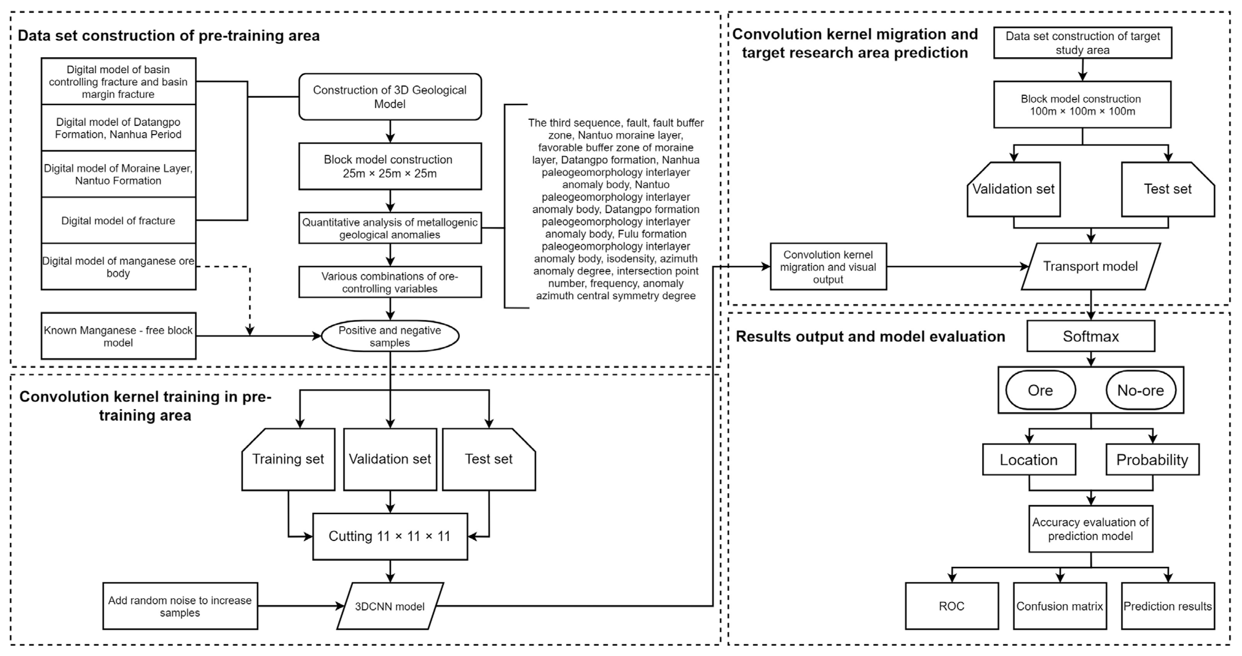
The overall framework of 3D metallogenic prediction based on the migration model proposed in this study is illustrated in
Figure 4, which mainly includes four parts.
Part one: Dataset construction of the pre-training area. The pre-training area generally refers to the area with detailed data. The data collected in this study mainly include 46 prospecting line profile maps of the Minle manganese mine and the Huomachong mining area, 90 map sections of the Minle manganese mine, 212 pieces of borehole data, the 1:100,000 lithofacies paleogeographic map of the Songtao-Huayuan area, the 1:10,000 topographic geological map of the Minle Manganese mine area, the 1:50,000 Heku geological map and Malichang geological map in western Hunan, Aster remote sensing data with a resolution of 30 m, and the detailed geological survey report of the Minle manganese mine. These data provide a strong basis for constructing a 3D digital model in the mining area. The data preprocessing procedure has been described in the previous section and will not be repeated here. To ensure the spatial similarity between the pre-training area and the target mining area, the overall shape and block proportion of the pre-training area should be consistent with the target area. Additionally, the attribute information of each block model should be consistent. Moreover, to ensure the effectiveness of the research, it is better to compare the conceptual model of the pre-training area with that of the target area and determine whether the key ore-controlling factors are consistent before training.
Part two: Convolution kernel training in the pre-training area. The transfer learning method adopted in this study outputs and transfers the parameters of the two convolution layers of the model by training with data of the pre-training area. As there are no relevant parameters in the pooling layer and dropout layer of the model, only the parameters of the convolution layer need to be transferred. Among the preprocessed positive and negative samples, 80% are taken as the training set and 20% as the validation set. To enhance the validity of the model, this study enlarges the sample size by adding random noise. The block model is stored in a central point way. Each centroid point is expanded in all directions by 5 points, respectively, which is composed of 11 × 11 × 11 particles. Different attributes of each sample block are input into the model, and the spatial distribution characteristics of the factors in the detailed data area are exploited to train the convolution kernel of the model by utilizing the excellent spatial feature extraction ability of the network structure.
Part three: Convolution kernel migration and prediction for the target study area. The dataset construction method for the target study area has been described in the previous section and will not be repeated here. The framework of the migration model is consistent with that of the pre-training model. The parameters of the pre-trained two-layer convolution kernel are output and visualized and then transferred to the model of the target study area for model verification. The potential correlation of spatial distribution of all input ore-controlling factors and the mineralization is implied. Finally, two classes of scores, namely the ore-containing score and the ore-free score, are obtained for each test sample on the target test set by the migration model, respectively.
Part four: Output result prediction and model evaluation. The output score of the fully connected layer is normalized by the Softmax layer, and finally, a score between 0 and 1 is obtained, which is the ore-containing and ore-free probability. Two indexes, i.e., accuracy and loss, are used to test the classification accuracy of 3D CNN models under different factor combinations. Meanwhile, the ROC curve and the confusion matrix are applied to evaluate the accuracy of the prediction model. By comparing the model evaluation results under different factor combinations, the best combination of predictive factors is obtained, and the corresponding prediction results are output. The position of each block is determined by coordinates for 3D model visualization.
Through the above technological method, the mineral prediction data in the study area with incomplete information, and the space distribution characteristics of the area with rich data, the potential relevance of the training classification model can be intelligently processed, thus allowing for deep mining predictions in the target study area and obtaining the localization and probability from the 3D prediction process.
3.1. Construction of Large Spatial Database
In the study of metallogenic prediction, the accurate, systematic, and comprehensive sorting of basic data in the study area is the basis and premise of model construction. The basic data of the study area during the preparation stage of the metallogenic prediction study should be collected and sorted and a detailed basic database of the study area needs to be constructed, thus laying the foundation for establishing an accurate model in the follow-up work. The basic data in the study area mainly consist of text data, two-dimensional data, and three-dimensional data.
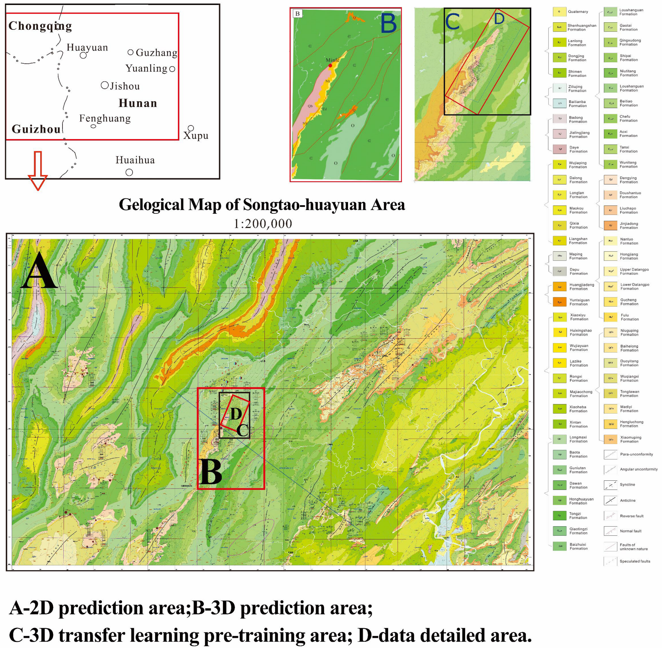
To address the issue of incomplete basic geological data in the study area, the study area was divided into the “2D prediction area”, the “3D deep learning area”, and the “3D migration learning area” according to the actual degree of detail of the basic data in the study area, corresponding to the Songtao-Huanyuan area, the Huayuan area, and the Minle area, whose relative 2D and 3D positions are shown in
Figure 1. Specifically, Area A is a two-dimensional prediction area (Songhua-Huayuan), Area B is a three-dimensional deep learning area (Huayuan), and Area C is a three-dimensional transfer learning pre-training area (Minle). The degree of detail of the basic data in the three areas increases successively. All the data collected in each area were sorted to construct the spatial datasets of the three areas. Then, the spatial datasets of the three areas were integrated into the basic database of the study area. The spatial data after collation are listed in
Table 2,
Table 3 and
Table 4.
3.2. 3D Modeling and Prediction Layer Construction
Guided by the intelligent prospecting theory of cognitive maps and combined with various data mining methods, this study aims to conduct multi-scale metallogenic prediction for the Songtao-Huayuan manganese deposit area. A 2D regional metallogenic prediction based on the Alexnet network is carried out in Area A (Songtao-Huayuan), and a 3D deep metallogenic prediction is implemented by the 3DCNN algorithm combined with borehole data and the section data in Area B (Huayuan). With further progress in mineral prediction, it was observed that there are incomplete data in the 3D modeling area of Area B. This study employed Surpac software to explicitly model the variables related to mineralization. Most of the exploration lines and borehole data are concentrated in Area D (
Figure 1). Therefore, to obtain a better quantitative prediction of mineral resources and improve the prediction efficiency, the unknown hidden information of geological mineralization needs to be explored deeply. This study optimizes the basic principle of the classical convolutional neural network and takes Area C (the Minle mining area), which has a similar metallogenic background and metallogenic mechanism as the pre-training area, and applies a transductive transfer learning method to transfer the convolution kernel of the deep neural network for the pre-training area to the target study area, i.e., area B (the Huayuan mining area). Thus, the improved CNN contains the potential spatial correlation between the ore-controlling factors and the ore body in the training area, and this spatial distribution correlation can be transferred to the target study area. From another point of view, due to the diverse and complex geological characteristics, and their spatio-temporal variation, it is difficult to embed the quantitative study of the algorithm into the convolution kernel to improve the metallogenic characteristics of the training. The CNN algorithm is superior in efficiency and simplicity as a result of the shared weight. If the convolution kernel is changed directly, a simple model will involve hundreds of thousands of weight factors. In this case, the model cannot be operated manually due to the significant calculation amount. However, the model-based migration method overcomes this difficulty. When there is incomplete information between deep and shallow data in the study area, this method can still be used to transfer the convolution kernel from the rich data area to the poor data area.
Additionally, to solve the problems of limited training samples in metallogenic prediction, the loss of geological meaning, and the increase in CNN training difficulty caused by the traditional data extension method, this paper proposes a data expansion method suitable for the prediction of metallogenic prospect areas, which not only retains most spatial features of the data but also solves the problem of limited sample data. Hence, the convergence speed of the model is improved and the metallogenic prediction accuracy of the Songtao-Huayuan 3D modeling area is enhanced.
3.2.1. Modeling of the Pre-Training Area
The data collected in area D (the Minle mining area) include 46 pieces of prospecting line profile maps, 90 pieces of map cut profiles, 212 pieces of borehole data, a 1:100,000 lithofacies paleogeographic map of the Songtao-Huayuan area, a 1:10,000 topographic geological map of the Minle manganese deposit area, a 1:50,000 Heku-Mali geological map of the western Hunan area, Aster remote sensing data with a resolution of 30 m, and a detailed geological survey report of Minle manganese deposits, which provide a powerful tool for constructing a 3D digital model of the mining area.
According to the existing data of the Minle mining area and the prospective geological model constructed above, this study establishes 3D models for the surface, fractures, ore body, Nantuo moraine layer, and Datangpo area in the study area based on different ore-controlling factors (such as structure, ore body, and stratum) and constructs an prospective ore digital model for the Minle mining area (
Table 5). Since the borehole in Minle mining area has not hit any fractures, all the fracture entity models in this area are constructed according to 46 exploration line profiles and the topographic geological map of the Minle mining area.
Some ore-controlling factors, such as finer sub-members, sequence stratigraphy, and geomorphology under the Datangpo Formation in the Minle mining area, cannot be expressed by 3D digital models, so this study adopts 3D reconstruction mainly for the subparts of the ancient landform, the manganese-bearing rock series, the sequence stratigraphy, and the Datangpo Formation (
Table 6).
3.2.2. Construction of 3D Pre-Training Layer
The Minle manganese ore block model was constructed according to the statistics of the data in the study area combined with the digital model of the surface range (
Figure 5). To guarantee the smooth progress of transfer learning, the total number of model blocks in the small block model should be consistent with the large block model, and thus the unit block size was set to 25 m × 25 m × 25 m. The model includes 2,606,100 blocks, of which the total number of positive samples is 1560 blocks and the total number of negative samples is 1450 blocks, and each unit block is endowed with the attributes in the prospective geological model (modeling area X
max = 635,975, X
min = 630,025; Y
max = 3,147,062, Y
min = 3,137,937; Z
max = 450, Z
min = −350).
According to the 3D weight of the evidence method, the evidence weight of each factor in the study area is shown in
Table 7, which intuitively reflects the relationship between various factors and mineralization.
The process of 3D modeling and construction of the prediction layer of the target study Area B (Huayuan mining area) has been described in the previous research [
29].
3.3. 3D CNN Modeling
3.3.1. 3D CNN Algorithm
Generally, 3D CNN adopts 3D convolutional layers, 3D pooling layers, and dense layers to extract images, and then it obtains a score by connecting a Softmax layer [
30,
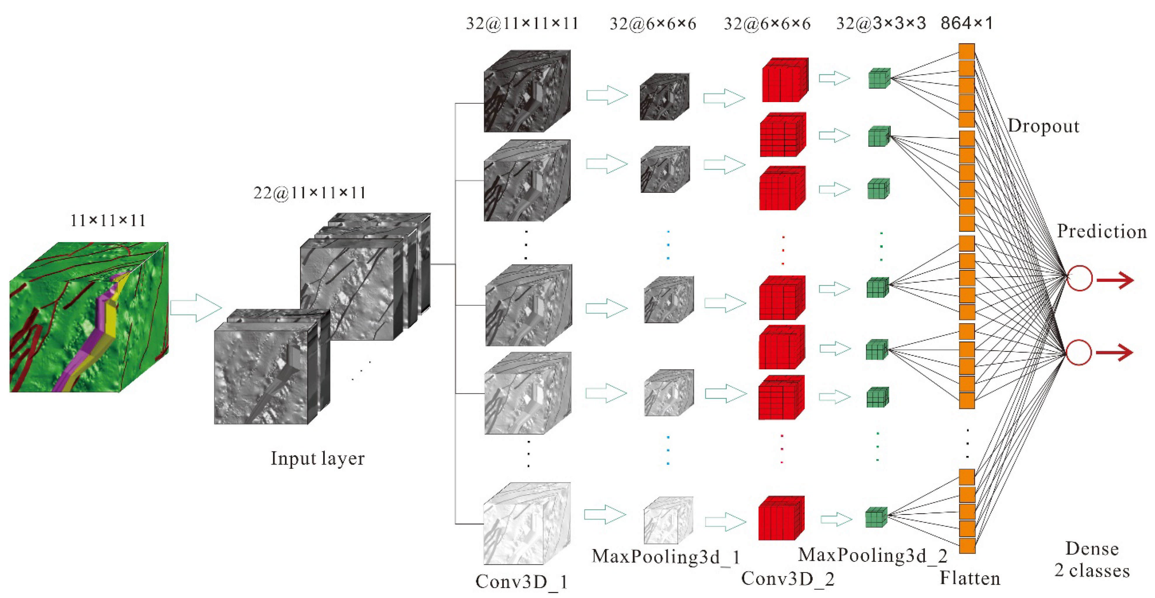
31]. In addition, each layer has several channels, and each channel represents a type of feature. In a 3D CNN, convolution and pooling is actually a cubic 3D characteristic block. Unlike 2D features, 3D features are presented as a set of neurons in a 3D form. In this study, the 3D spatial distribution of the 22 ore-controlling factors is taken as the input of the 3D CNN prediction model, then the ore-bearing probability of each voxel can be obtained after the processing of two convolutional layers and two pooling layers, as well as the flatten layer, dropout layer, dense layer, and Softmax layer (
Figure 6). The specific principle of the 3D CNN model has been shown in previous research [
29].
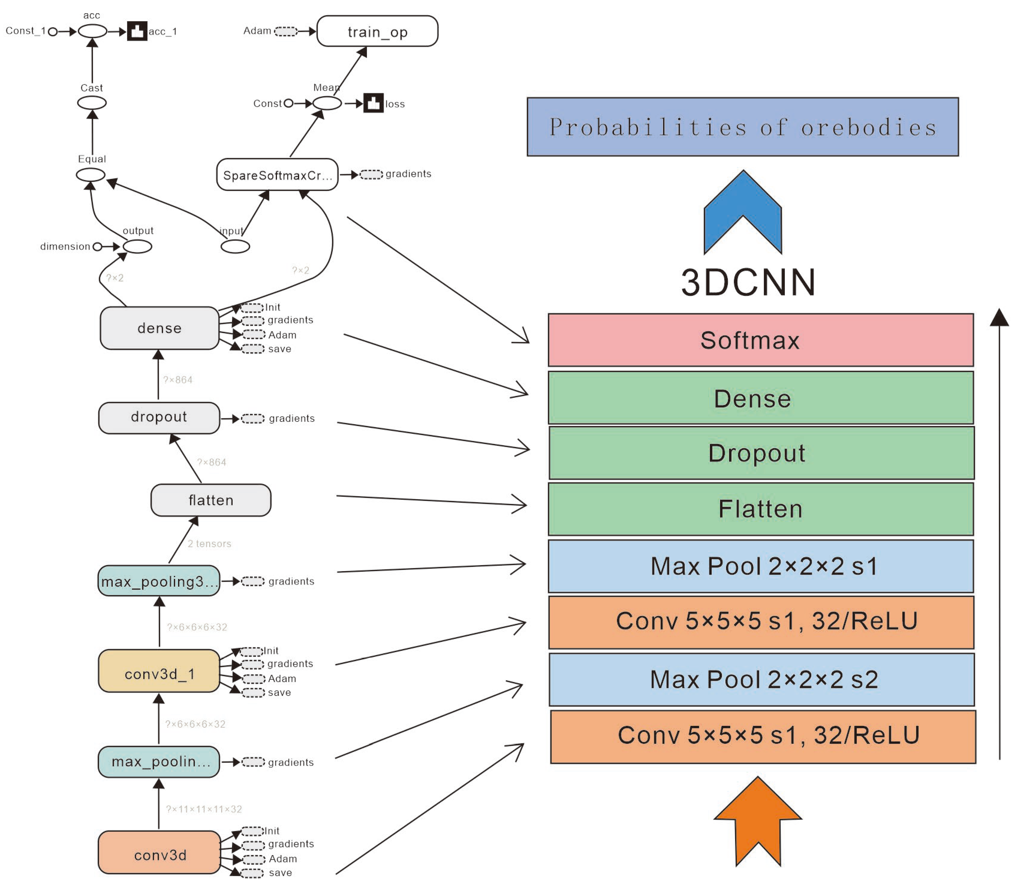
The super-parameter settings for each layer of the 3D CNN model adopted in this study is shown in
Figure 7. (1) The first layer (convolutional layer): the size of the convolutional kernel = [5,5,5], stride = [1,1,1], output channel = 32, and padding = same (expanded edge, the input equals to the output). (2) The second layer (pooling layer): pool_size = [2,2,2], stride = [2,2,2], output channel = 32 (default), and padding = same. (3) The third layer (convolutional layer): the size of the convolutional kernel = [5,5,5], stride = [1,1,1], output channel = 32, and padding = same. (4) The fourth layer (pooling layer): pool_size = [2,2,2], stride = [1,1,1], output channel = 32, and padding = same. Each convolutional layer contains the ReLU activation function, and subsequently the downsampling operation (i.e., pooling processing). As the activation function of the CNN, ReLU outperforms Sigmoid in terms of the verification effect in the deeper network, and it can solve the gradient diffusion problem faced by Sigmoid in the deeper network. Subsequently, the output results of the 3D CNN are fed into the dense layer after the flatten operation, and the process of preventing overfitting of the dropout layer is imposed on the subsequent dense layers. Finally, the ore-bearing probability and non-ore-bearing probability of each block can be obtained through the Softmax operation.
3.3.2. Localization and Probability Determination
By acquiring the coordinates of the prediction results, the predicted ore-bearing areas and the areas developing known deposits (occurrences) are given different colors for outputting, and the output results are saved in the CSV format. Meanwhile, the ore-bearing probability can be determined by the Softmax activation function, where the details are described in
Section 3.2.1. However, the Softmax activation function can only be applied to a neuron with more than one output, and it guarantees that the sum of all the output neurons is 1.0, so the output is a probability value less than or equal to 1, which makes it easy to compare various output values. Regarding
as the ore-bearing or non-ore-bearing “probability”, for example, if the output of type A “ore-bearing” is 0.8, it can be considered that the ore-bearing probability of the area delineated by the prediction model is 80%.
3.4. Transfer Learning Model
Compared with machine learning’s automatically exploration of knowledge from data to address instant issues, transfer learning, as a significant branch of machine learning, is the process of transferring a model from the previous domain to a new one in accordance with the similarity of the task, model, or data. Since data or tasks are correlated in applications, the already trained model parameter (knowledge) is transferred to a new model to increase its convergence speed and learning efficiency, and the new model does not start from scratch. Zhang Ye et al. realized the automatic identification and classification of rock lithology with transfer learning, which provided a new approach for the automatic classification of rock lithology, and its robustness and generalization abilities were verified [
23]. The most important issue of transfer learning lies in the detection of the similarity of two domains, and the task can be completed after similarity confirmation.
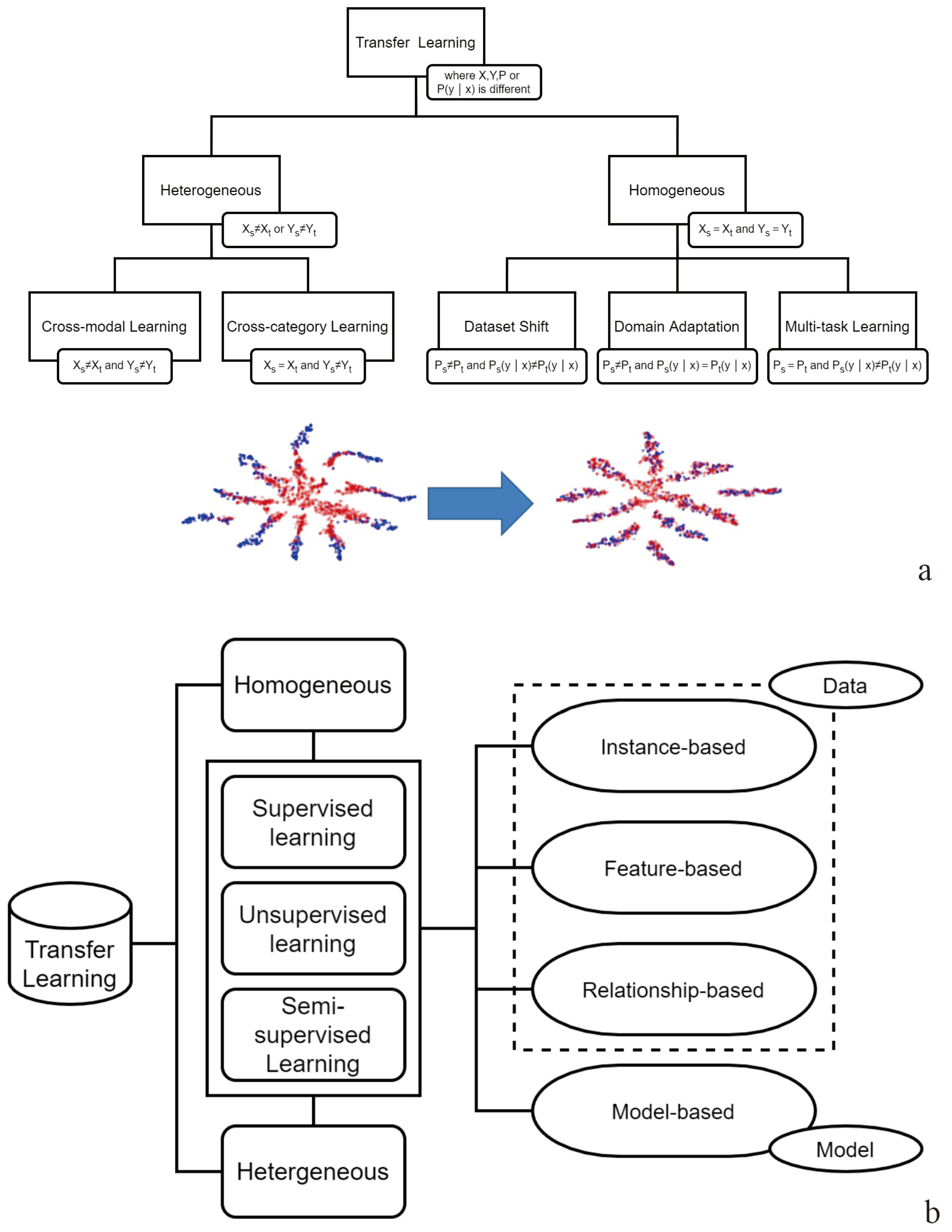
The domain and task are two important concepts of transfer learning; the former is identified as a special field and data features differ in different fields, and thus the task can be considered the target of business scenarios. For instance, emotion recognition and automatic question answering are two different tasks. Thus, data for different tasks may originate from different domains. Transfer learning is a type of solution philosophy rather than a specific algorithm. The detailed transfer learning process comprises two steps: (1) pre-training is conducted on the model based on super-sized data and (2) fine adjustment (on weight or terminal structure) is performed according to a specific task. There exists heterogeneous transfer learning and isomorphic transfer learning, named for whether the feature space and label space are identical (
Figure 8a). According to the method used, there is instance (sample)-based transfer learning, feature-based transfer learning, parameter (model)-based transfer learning, and relationship-based transfer learning (
Figure 8b). In this study, model-based transfer learning is adopted for mineral prediction.
3.4.1. Sample Data Expansion
Data expansion refers to the application of a series of deformations on a group of marked training data to obtain diversified training data for sample expansion. Many sample expansion methods have been proposed, including flipping and rotation [
32], shearing and scaling [
33], and changing the intensity of the RGB channel [
34]. The most important principle of sample expansion is that the adopted deformation will not change the label meaning of the sample [
35], the frequently used data expansion methods such as flipping and rotation of geological data may change the data direction. These methods are likely to generate a new direction of faults and intrusive rocks, which are either irrelevant to mineral deposits or beyond the study area. Consequently, such expansion seems to be invalid and may increase the training difficulty of the CNN prediction model.
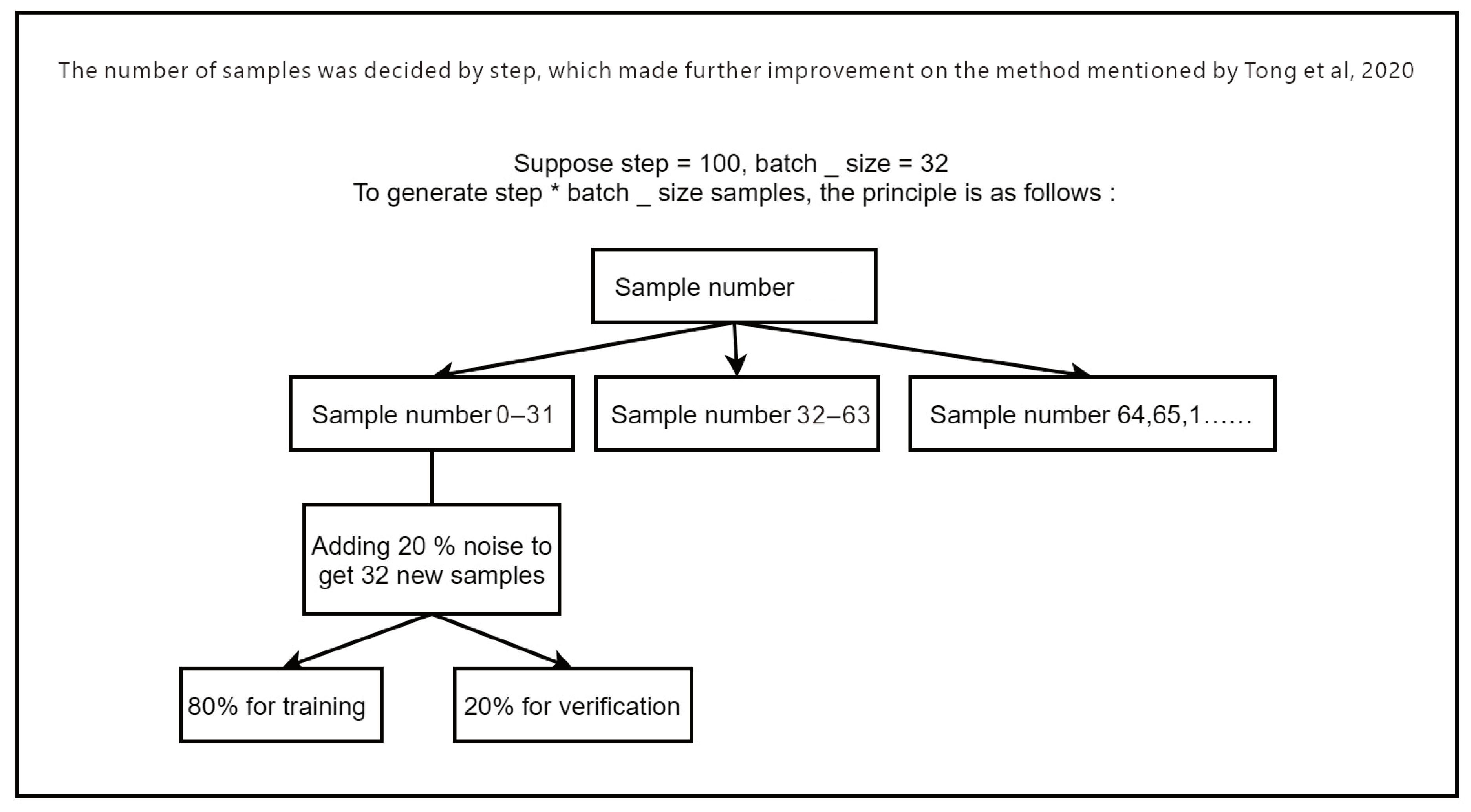
A sample expansion method for metallogenic prediction is proposed in this study which ensures the diversification of expanded data and maintains the geological meaning. The basic principle of such a method is to add random noise to the sample data while reserving the geological meaning of the data. In contrast to most previous metallogenic prediction research, CNN focuses on spatial distribution and data correlation instead of the value of a specific point. Thus, most spatial data features contain noise, and there are insufficient training samples for metallogenic prediction driven by data. Unlike picture processing, the data in mineral prediction are hindered by geological meanings. For instance, a ridiculous scenario of significant spatial difference between two neighboring points and a specific fault may appear. Therefore, this study proposes an approach to expand sample data based on random noise, and its validity in the CNN model has been previously proven [
36]. This study has made some modifications, and the principle of the proposed approach is presented in
Figure 9:
Step 1: The dropout value of the noise scale is set to 20.0% in this study. Step 2: Sample data are captured as shown in
Figure 9; the step is set to 100, batch_size is 32, and the sample number is 0–65. There are 66 recognized samples in total, 32 of which are randomly iteratively selected. Step 3: Random noise samples are developed, and Gaussian distribution is applied to acquire noise distribution. A total of 20% of all samples are in the study area, and 32 samples iteratively selected each time are imposed with random noise distribution to develop 32 new random samples, 80% of which are adopted as training data and the rest are verification data. Steps 2 and 3 are repeated, and the maximum step*batch-size samples will be obtained until there are sufficient positive and negative samples to train the CNN model.
3.4.2. Operating Characteristic Curve
As one of the visible methods to evaluate the performance of classifiers, the receiver operating characteristic curve (ROC) is widely used in geochemical anomaly and mineral resource qualitative prediction [
37,
38,
39,
40]. The abnormal distribution of model prediction is compared with known mineral deposits (points), and their spatial relationship is measured generally by statistical indicators such as
AUC (area under the curve),
ZAUC (Z-area under the curve), etc.
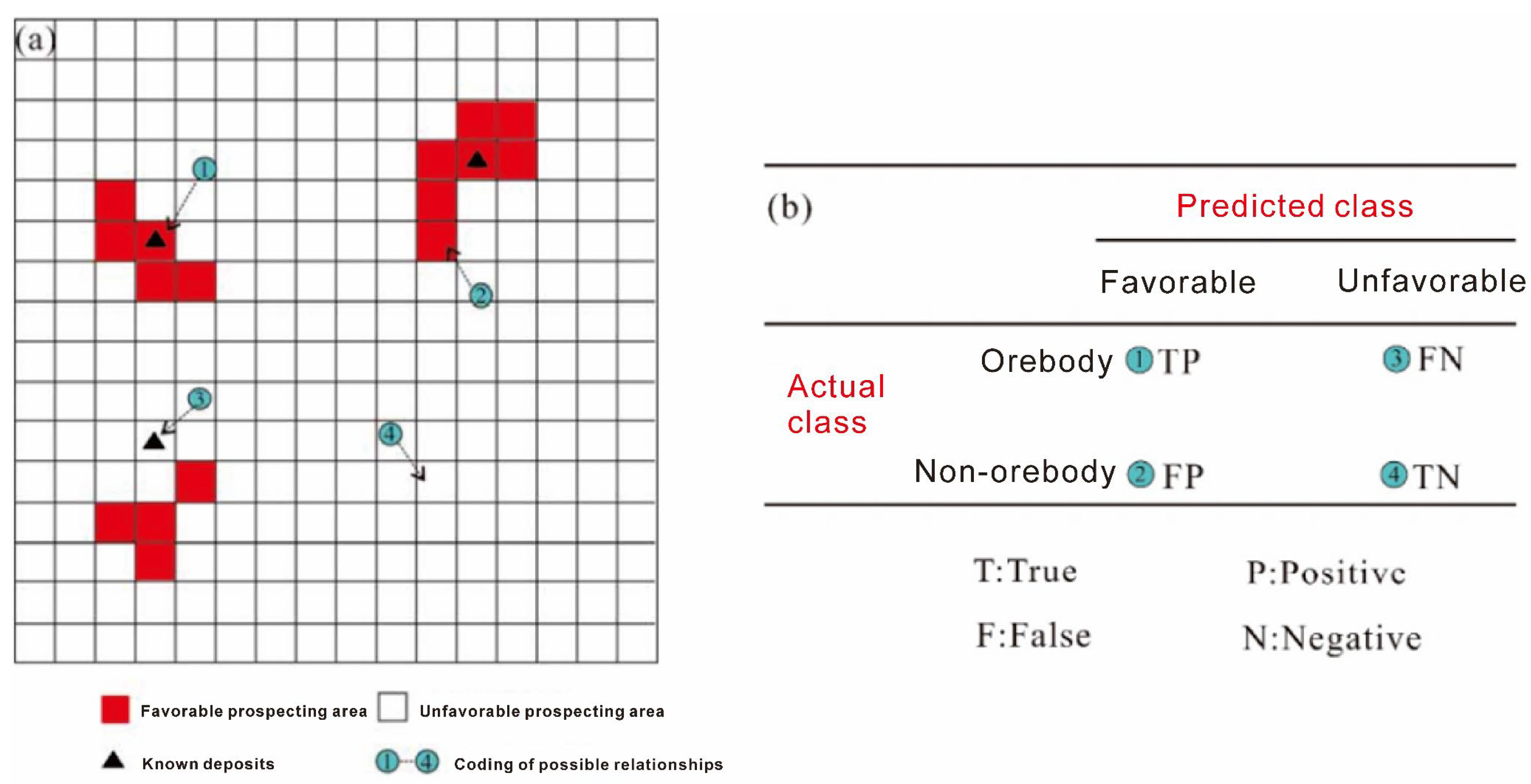
Figure 10a shows the spatial relationship between the predicted classification result and mineral distribution in four categories: (1) mineral exists in reality and in the prediction (
TP); (2) mineral exists in reality but not in the prediction (
FN); (3) mineral exists in the prediction but not in reality (
FP); (4) mineral neither exists in reality nor in the prediction (
TN). Finally, a confusion matrix is established, as shown in
Figure 10b.
In the ROC, different threshold values are defined and one threshold is selected each time to obtain an
FPR (False Positive Ratio) and
TPR (true positive ratio), with the former on the horizontal line and the latter on the vertical line, connecting numerous points to develop the blue curve in
Figure 10a. The calculation formulae of
FPR and
TPR are shown below [
42]:
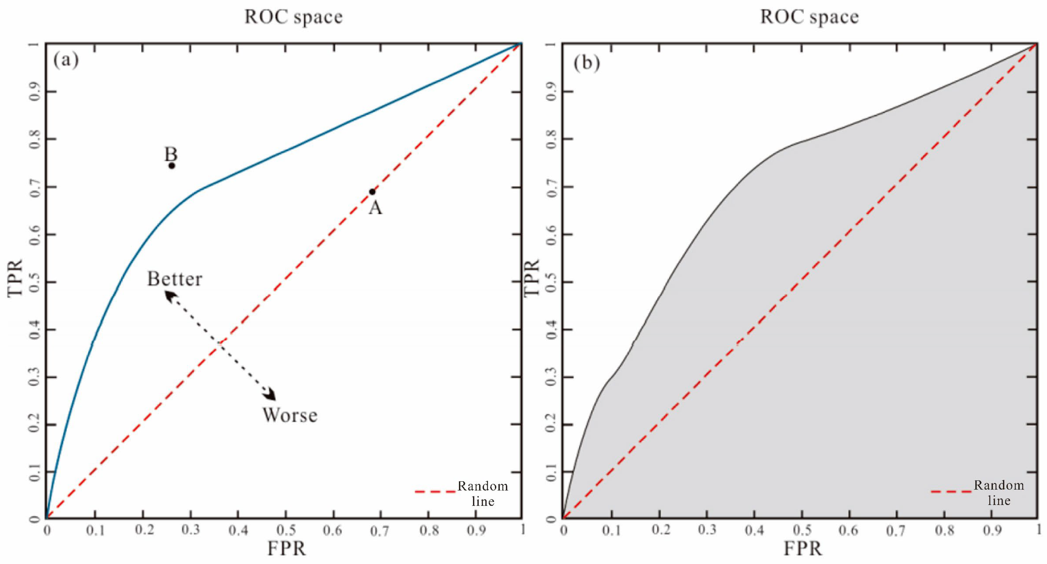
In the ROC shown in
Figure 11a, the red dummy line linking (0, 0) and (1, 1) is random, the point (A) equates to a random process when
TPR =
FPR, and the point (B) above the line indicates that
TPR >
FPR, where the probability that the mineral exists in both reality and in the prediction is higher than that of the mineral existing in the prediction but not in reality. The closer the ROC approaches the point (0, 1) in the upper-left corner, the better the prediction efficiency of the prediction model towards predicting known mineral deposits (points).
To conduct a qualitative evaluation of classification performance, the
AUC formed by ROC and the coordinate, e.g., the gray part in
Figure 11b, can be calculated. Then, the predicted results of the model can be qualitatively compared based on the
AUC [
43]; an
AUC of >0.5 indicates better prediction results than the random process and an
AUC of <0.5 indicates a better random process than the predicted results. The higher the value, the better the prediction results [
44]. The calculation formula of the
AUC is as follows:
where,
.
The calculation formula of the
AUC standard deviation,
, is as follows:
where,
This study performs a comparative analysis of the performance of the transfer learning model and the 3DCNN model under different factor combinations via the ROC and the confusion matrix to determine the optimal factor combination and prediction method.
4. Results and Discussion
This study employs a transfer learning method to transfer the pre-training area to the output and transfer the two convolution parameters of the model. As the parameters of the pooling and dropout layers in the model are irrelevant, only the parameters of convolution need to be transferred. A total of 80% of pre-processed positive and negative samples are taken as the training set and the remaining 20% are used as the validation set. Meanwhile, random noise is added to increase the sample size for higher model validity. The block-model-centered storage extends the center of mass forwards, backward, left, and right by 5 points, leading to 11 × 11 × 11 mass points. Different attributes of each sample block are input into the model, and the convolution kernel of the model is trained by the distribution feature of space elements with the assistance of the outstanding spatial characteristic extraction capability of such a network structure.
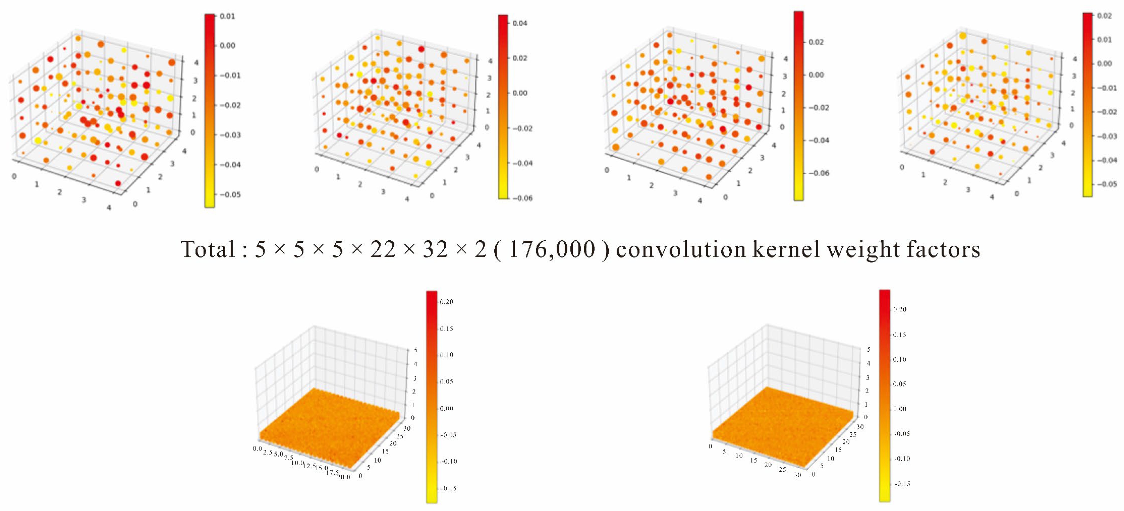
The pre-trained parameters of two convolution kernels are output and visualized to perform model verification after they are transferred to the target study area. In this process, the potential links between the spatial distribution of all inserted ore-controlling factors and metallogeny are included. For each test sample, two values (containing minerals and not) are obtained by the transfer model for the target test set. The pre-trained convolution kernel is rendered according to weight, and the size of each convolution kernel is 5 × 5 × 5, with the input channel shown in
Figure 6 (the structure of the 3DCNN prediction model), where there are 22 prediction stratums and 32 output channels in total. Therefore, 176,000 weight factors of convolution kernels are output, and they are arranged as a 5 × 5 × 5 cubic, as shown in
Figure 12.
4.1. Comparison of Different Factor Combinations
A contrast test was carried out on six groups of twenty-two ore-controlling factors, with comprehensive prospecting prediction applied by transfer learning and the 3D CNN to obtain the optimum ore-controlling factor combinations by comparing the training accuracy, training loss, validation accuracy, and validation loss of the prediction models trained on different factor layers, with the results shown in
Table 8. Meanwhile, a comparative analysis was conducted on transfer learning, and the prediction results of the 3D CNN were exploited to evaluate the feasibility and superiority of transfer learning methods in 3D metallogenic prediction.
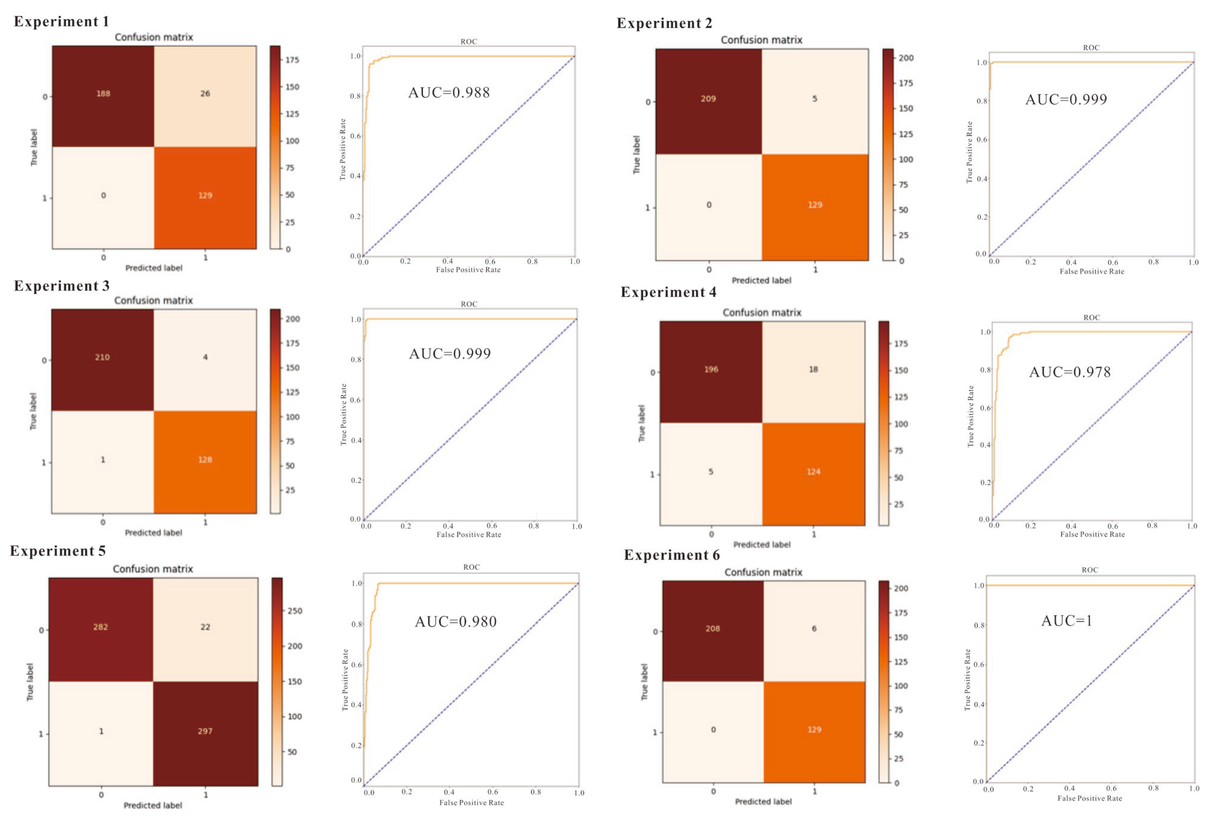
Based on the evaluation of six groups of prediction models under transfer learning and the development of the confusion matrix and ROC curve of these models, it is indicated that the ROC curves of all models approach the upper-left corner point (0, 1), demonstrating the excellent prediction performance of these models towards known mineral deposits (points). Then, a qualitative evaluation of classification performance was realized by the
AUC formed by the ROC and the coordinate (
Figure 13). The
AUC values of all six groups of prediction models are above 0.5 and close to 1, indicating that the prediction models are appropriate because of their advantages over random models in terms of prediction capacity. Specifically, the best and worst prediction performances were obtained in test 6 and test 4, respectively, with the latter’s
AUC equaling 0.978 with the factor combination 1–13. Compared with test 4, test 5 deletes factor 13 of the Fulu Fm ancient landform interlayer anomalies, and it exhibits a stronger prediction ability.
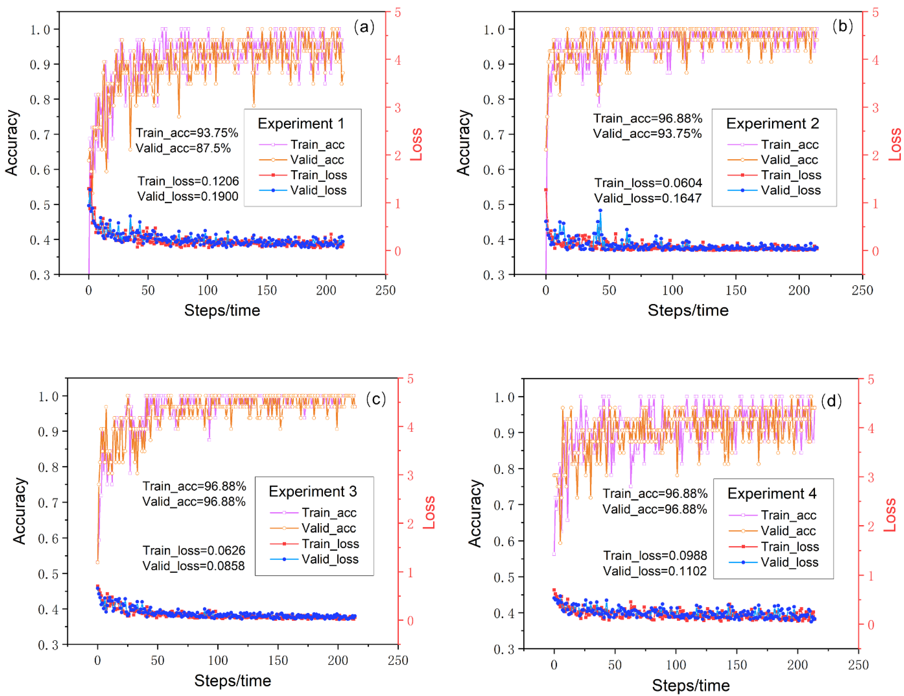
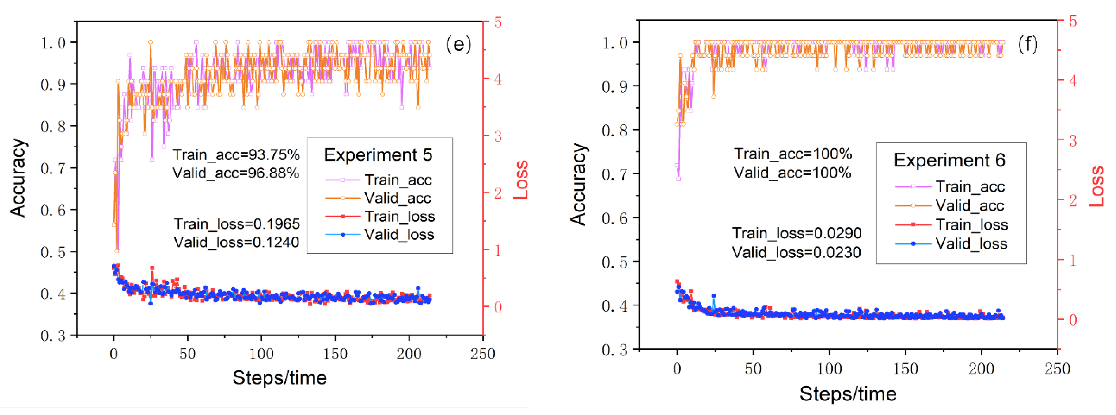
According to a comparison analysis (
Figure 14) of the training loss, training accuracy, validation accuracy, and validation loss of the six groups of transfer learning models, it can be observed that the curve of the final model reaches convergence, and the loss value approaches 0. The highest training accuracy and validation accuracy reach 100%, and they are obtained in test 6, which shows the optimum prediction performance and stability, with the factor combination ranging from 1–6 (the third sequence, the stratum of the Datangpo Formation, the favorable metallogenic buffer zone of the Nantuo moraine layer, the interlaminar anomalous body of the ancient landform of the Datangpo Formation, the interlaminar anomalous body of the ancient landform of the Nantuo Formation, and the interlaminar anomalous body of the ancient landform of the Nanhua Period). Among these six tests, the worse prediction performance appears in test 1, and in this test, the training accuracy was 93.75%, the validation accuracy was 87.5%, the training loss was 0.1965, and the validation loss was 0.1240 when the factor combination ranged from 1–22, indicating that interference factors affect the test results in 22 ore-controlling factors.
4.2. Comparative Test on 3DCMM and TL
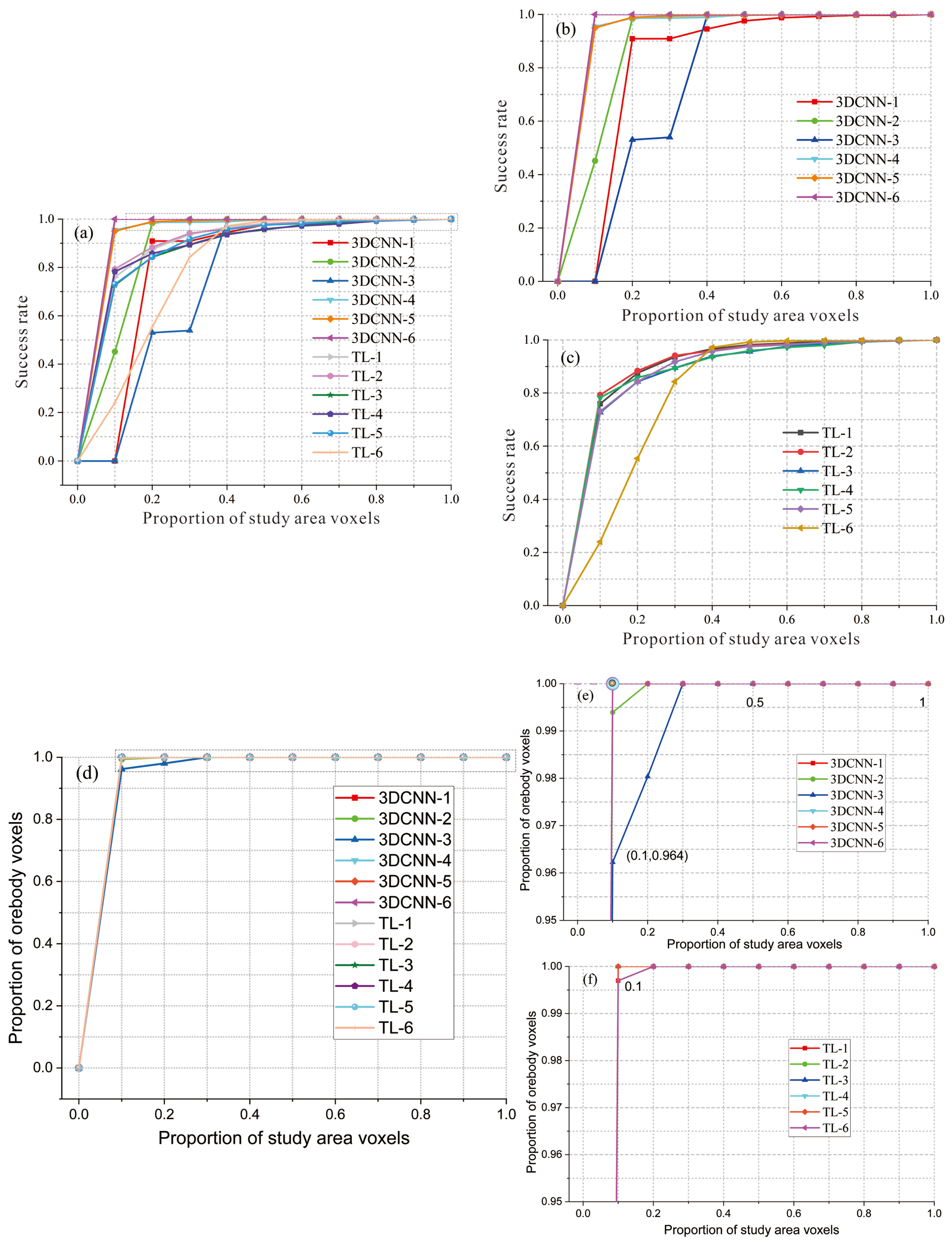
By plotting the success rate curves and ore-controlling rate curves, this study further quantitatively evaluated the performance of the 3D CNN model and the 3D CNN-TL model (
Figure 15). It is worth mentioning that there are differences between the predicted results and the results obtained by the calculation method of the 3D CNN, since both models have generated random noise via a Gaussian distribution to increase the sample quantity. The calculation process of the success rate is described as follows: firstly, the predicted ore-bearing probability of all the blocks in descending sequence is obtained and the blocks with the predicted ore-bearing probability greater than or equal to 0.5 are extracted. Then, the extracted probability is reclassified by setting various thresholds. Finally, the success rate is calculated by conducting statistics on the number of known blocks in various segments [
45]. The calculation process of the ore-controlling rate involves conducting statistical analyses and calculations of all blocks in the study area.
In
Figure 15a,d, the success rate curves and ore-controlling rate curves of 12 tests are presented, indicating that the success rate of the CNN model (3D CNN-TL) in tests 1–5 exceeds 70% at a threshold value of 10% after transfer learning, while only the last three tests for the 3D CNN model reach a similar level. In other words, the first 10% of minerals predicted by the 3D CNN-TL model cover more than 70 known minerals. It is obvious that the 3D CNN-TL outperforms the 3D CNN in the predicted results, and there is a big discrepancy in the convergence of different tests and a significant difference in the growth of convergence. In contrast, the convergence of the 3D CNN-TL model is much smoother, and the overall tendency of factors in different groups is similar. Under the influence of Gaussian noise, the 3D CNN-TL model maintains stable predictions with strong robustness (
Figure 15b–c). A comparative analysis on different test groups indicates that test 4 and test 5 achieve the best performance regardless of the model. The ore-controlling factor combinations for test 4 are 1–13 while for test 5, they are 1–12.
In
Figure 15d, the ore-controlling rate curves reveal that the ore-controlling rate exceeds 95% at a threshold value of 10%. To further investigate the differences in all 12 tests, this study analyzed the variation tendency (
Figure 15e–f) of ore-controlling rates in different tests by selecting the ore-controlling rate between 95% and 100%. In
Figure 11f, all known ore body blocks are contained in the blocks of the top 20% with ore-bearing potential in the 3D CNN-TL, while only 98% of blocks are included in the blocks of the top 20% with ore-bearing potential in the 3D CNN. The prediction result of the 3D CNN model includes all known ore body blocks only when the threshold value reaches 30%. However, the convergence rapidity of TL-6 is slower than other groups regarding the success rate curves and ore-controlling rate curves in transfer learning models. Therefore, ore-controlling factors containing 1–6 in test 6 may be unsuitable for applications in transfer learning models.
To sum up, the transfer learning prediction model demonstrates high stability and convergence rapidity, since five tests achieve a good performance. The exception is test 6, which has lower convergence speed but the highest prediction accuracy of 100%.
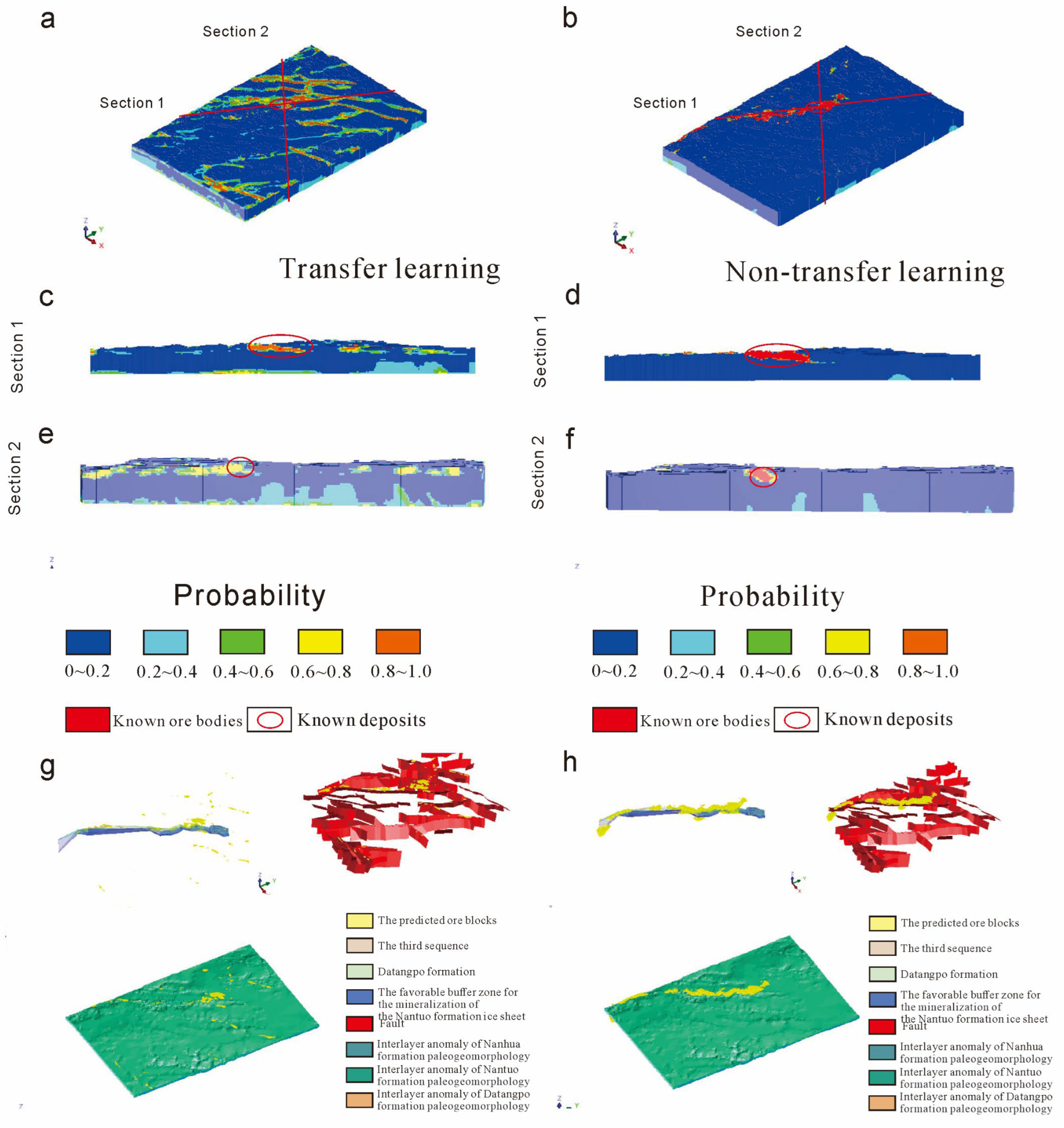
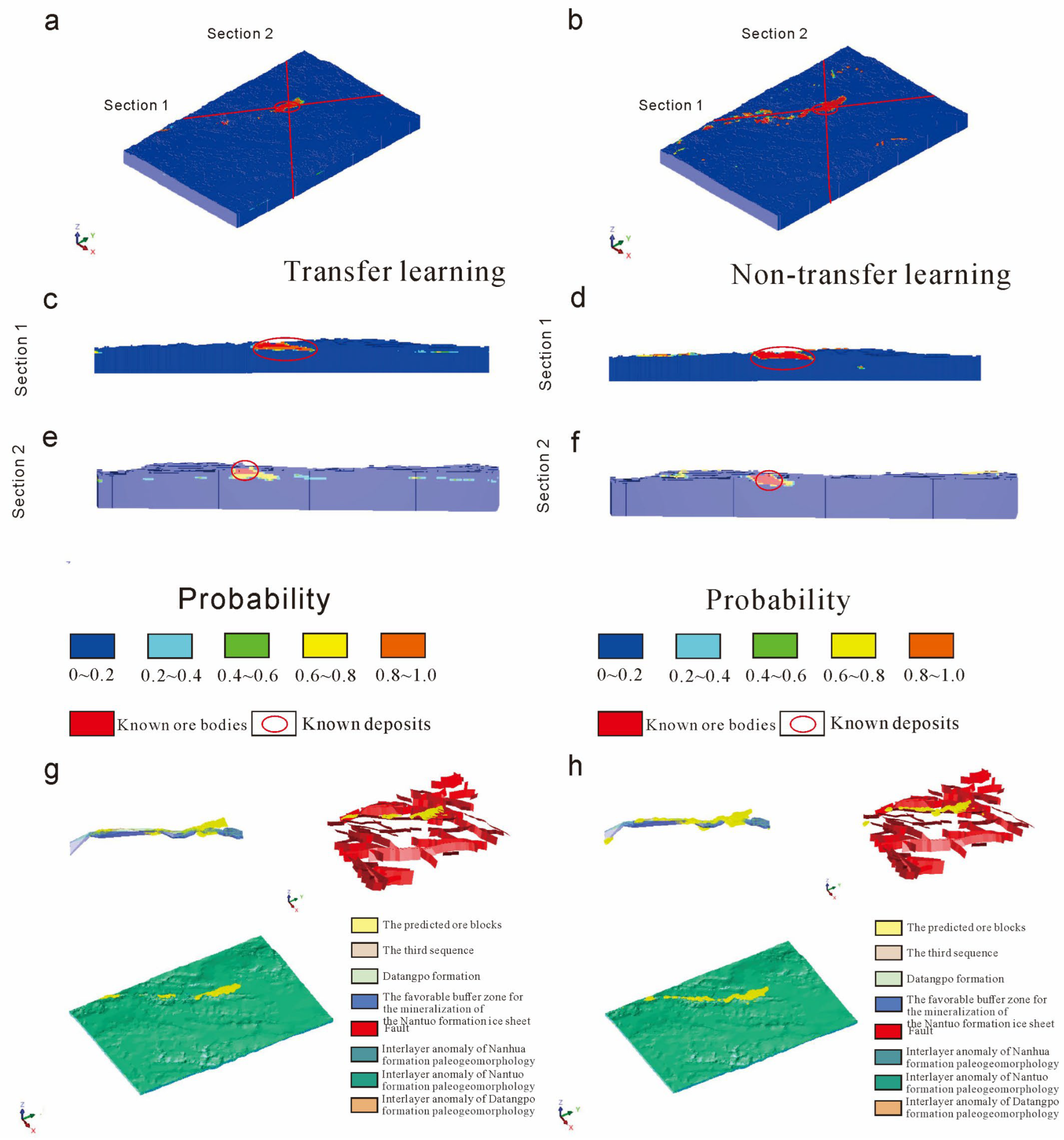
Based on a comparative analysis of the prediction probability distribution and prediction results of the 3D CNN model and the WofE model with different ore-controlling factors in six groups, it can be concluded that the 3D proof layers 1–12 and 1–6 included in test 5 and test 6 contribute to a superior performance. Three-dimensional metallogenic prospects (
Figure 16 and
Figure 17) were developed by 3D CNN and 3D CNN-TL prediction models using the same dataset, block size, and variable. On the Earth’s surface, the blocks of a high probability rate are mainly distributed in places where Datangpo formation appears (
Figure 16a,b and
Figure 17a,b). In profile, the known ore bodies of test 5 and test 6 are firmly embraced in blocks with a 3D CNN prediction probability ranging from 0.8–1.0 (
Figure 16c,e and
Figure 17c,e). The predicted ore is widely distributed, while the probability of other non-predicted areas is much lower. However, there are many seriously faulted predicted ore blocks under the probability range of 0.5–0.7 in the transfer learning results of test 5. This is because prediction factors 7–12 are faults and different areas of fault buffer zones, which affect the predicted results of the model. Thus, the predicted results of test 6 are better, where the combination of ore-controlling factors is 1–6 (the third sequence, the stratum of the Datangpo formation, the favorable metallogenic buffer zone of the Nantuo moraine layer, the interlaminar anomalous body of the ancient landform of the Datangpo formation, the interlaminar anomalous body of the ancient landform of the Nantuo formation, and the interlaminar anomalous body of the ancient landform of the Nanhua Period). However, the 3D CNN performs better under the same factor conditions, as shown in
Figure 16b–f. After integrating the predicted results of ore bodies based on an intelligent algorithm with 12 ore-controlling factor layers, it can be seen that predicted ore bodies exist in the third sequence (the stratum of the Datangpo formation, the favorable metallogenic buffer zone of the Nantuo moraine layer, the interlaminar anomalous body of the ancient landform of the Datangpo formation, the interlaminar anomalous body of the ancient landform of the Nantuo formation, and the interlaminar anomalous body of the ancient landform of the Nanhua Period) and beside faults. Thus, these blocks are areas of high prospective potential (
Figure 16g,h and
Figure 17g,h).
Further study on test 6 with a better prediction effect (
Figure 17) indicates that the prediction results of the non-transfer learning model are relatively disperse (
Figure 17b–f) due to a large number of predicting blocks and the absence of known ore blocks in some of the high-valued areas. In comparison, the prediction of the transfer learning model is concentrated, and the predicted area includes ore blocks, while known ore areas extend peripherally. Therefore, the transfer model is advantageous in prediction under the factor combinations of test 6.
To sum up, ore-controlling factors of 1–6 are superior, while those of 1–12 in the fault layers significantly affect the learning results. The 3D CNN model performs well with no disturbances and realizes accurate prediction. With the ore-controlling factor combinations of 1–6, the transfer learning model is better because of the scarcity and concentration of high probability blocks predicted. Thus, the 3D prediction method based on transfer learning in this study is feasible and accurate.
4.3. Comprehensive Analysis of Prediction Results
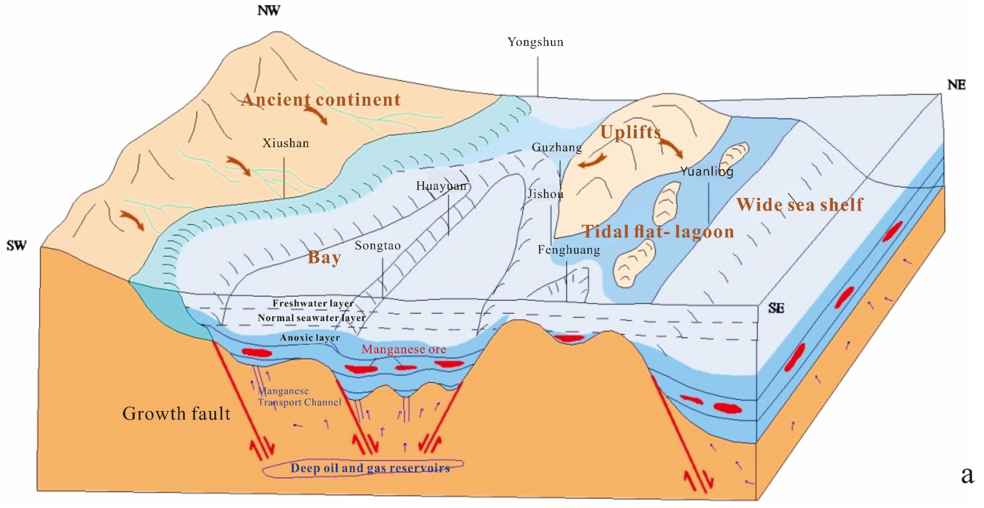
According to a study on the genetic types of Datangpo-type manganese ore in the Huayuan area, the metallogenic model of ancient manganese ore gas leaks in the rift basin is one of the most important genetic types in this area [
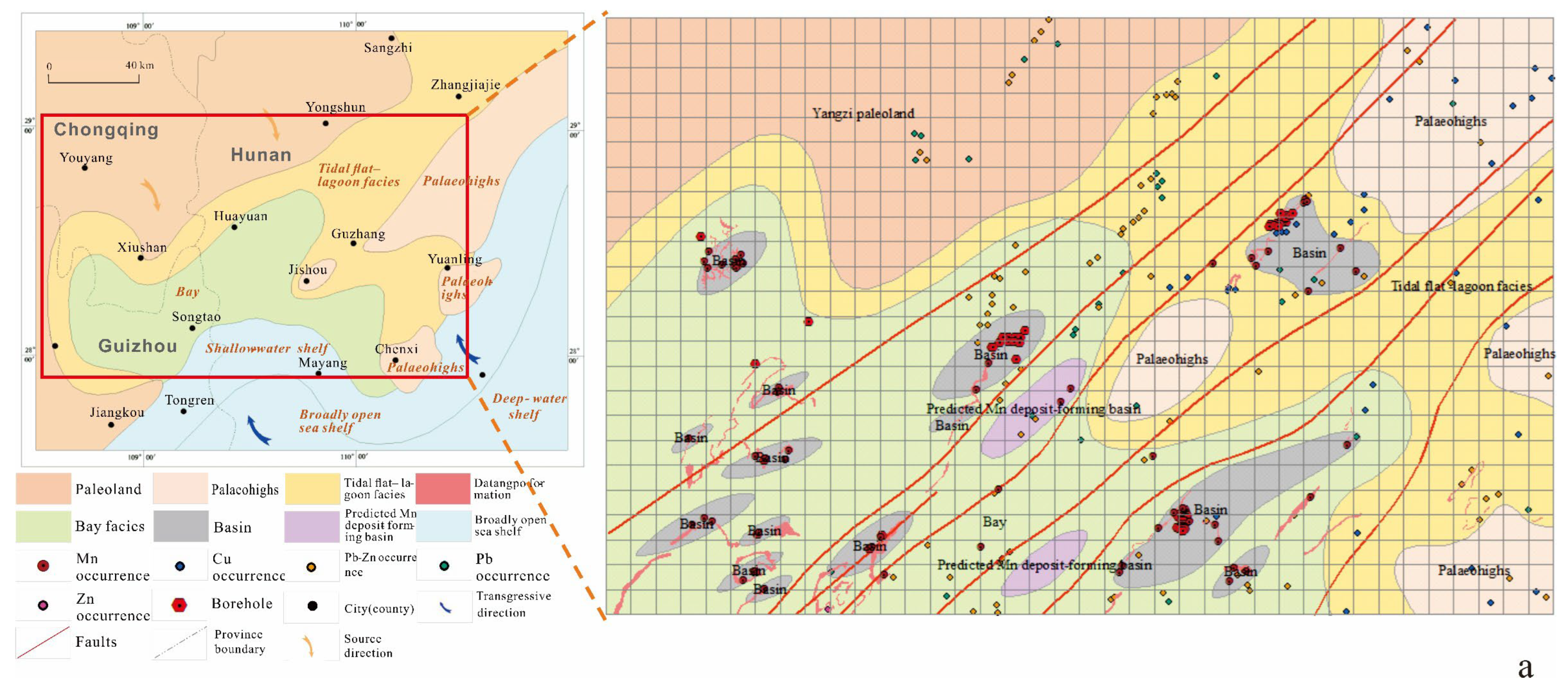
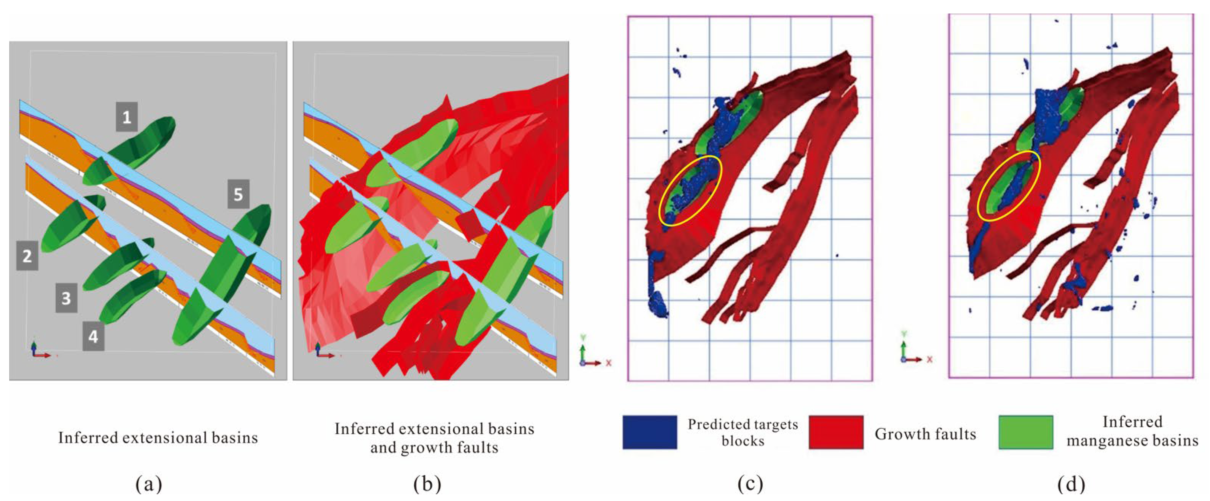
25]. The location of ancient natural gas vents has a significant effect on the formation and production location of this type of manganese ore. The deep and large faults can serve not only as a favorable location for the ancient natural gas vents but also as the most favorable channel for hydrothermal migration and storage. Based on speculation, the growth fault model of the Nanhua Period is established in this study. In addition, the deep rift basin is responsible for the abundance of manganese sedimentary ore in Hunan and Guizhou. Therefore, the fault basins analyzed based on lithofacies were compared with the geophysical exploration data, the five basins were finally determined, shown in the following figure, and 3D models were constructed (
Figure 18a,b). However, the basin model and the growth fault model were established on the speculation of geological and geophysical materials, and thus cannot be applied as a variable (3D pre-training layers) in intelligent prediction, so overlaying the geological model with the predicted results has a certain validation significance.
After integrating the prediction results of test 5, which achieves the optimal model performance with the 3D CNN algorithm, with those of test 6, which achieves the best performance in transfer learning with the predicted growth faults and manganese basins (both are indispensable metallogenic factors for sedimentary manganese), it can be observed that the prediction results correspond to basin 1 and 2 to the highest degree. Since basin 1 is the already mined Minle manganese, its surrounding favorable districts are not identified as metallogenic prospects (the yellow circle). Meanwhile, there is a high coincidence between the delineated metallogenic prospect and the predicted manganese basin, with the former being located on the hanging side of the growth fault, providing the best metallogenic conditions. When the threshold value of the delineated prospect is 0.65, the prediction results based on transfer learning are dispersed in the east and south, which are not affected by the distribution of other basins. However, it converges between two basins as the threshold value increases, and there is some directivity in the prediction results which corresponds to the geological features of this study area, thus verifying the feasibility and validity of this intelligent prediction method.


