Modeling of Sand Triaxial Specimens under Compression: Introducing an Elasto-Plastic Finite Element Model to Capture the Impact of Specimens’ Heterogeneity

Abstract

This paper follows up on a series of reference papers that inspired MDPI’s Topic “Stochastic Geomechanics: From Experimentation to Forward Modeling”, where global and local deformation effects on sand specimens are fully described from high-resolution boundary displacement fields, as supported by a comprehensive experimental database (which includes varying degrees of specimen’s heterogeneity) that is available to the scientific community for further study. This paper presents an elasto-plastic comparative analysis of different finite element models reproducing different sand specimen heterogeneity configurations as follows: loose, dense, and half-dense half-loose specimens. The experimental conditions for these specimens’ heterogeneity configurations were simulated with an axisymmetric finite element model. To characterize the stress-strain response obtained from the experiments, an elasto-plastic constitutive model with strain-hardening and softening laws was adopted to reproduce the sand specimens’ mechanistic response. An expert-based calibration of the numerical models accounted for both global and local effects by making use of global observations captured by the triaxial point sensors (i.e., axial force and displacement) and by local observations captured by 3D digital image correlation analysis (i.e., 3D boundary displacement fields). Results show that predictions of the proposed numerical models are in good agreement with the experimental observations, both global and local responses. The combined use of global and local observations to calibrate sand triaxial specimens sets the basis for a more comprehensive parameterization process. For the first model set, three experiments were assumed with homogeneous materials. While both dense and loose models showed good agreement with the experiments, the displacement field prediction of the half-dense half-loose layered model identified limitations in reproducing heterogeneous configurations. Afterward, the second set compared and analyzed the half-dense half-loose layered models by implementing a heterogeneous model, showing significantly better model predictions (i.e., after the implementation of the heterogeneous model, which accounts for a transition zone between the upper and lower segments).

1. Introduction

Four reference papers [1,2,3,4] precede this work, one introducing the supporting experimental database used to carry out numerical analyses on local deformation effects discussed in this paper [1] and its companion paper that presents the statistical analyses of the experimental database [2]. The other two papers study the kinematics of local deformation phenomena observed on the boundary of triaxial compression tests [3] and their corresponding statistical analysis, respectively [4]. This paper presents a comparative analysis of the deformation and behavior of different sand specimens, including the following: dense, loose, and half-dense half-loose layered specimens. The objective of this work is to validate the use of a modeling methodology based on finite elements and the use of an elasto-plastic constitutive model, to capture both global and local kinematic responses observed during a triaxial compression test.

One of the key elements required for the mechanistic characterization of geomaterials is the determination of the most suitable constitutive model. This requires the formulation of a model and its corresponding calibration process, which depends on several conditions. For example, the ability of the model to capture the physics associated with the particular initial and boundary conditions, material characteristics, the easiness to implement it, and the availability of a numerical solver to simulate the material behavior [5,6,7,8,9]. Therefore, the proper selection of a constitutive model lies in its capacity to simulate the material’s states of deformation and strength while providing a sound phenomenological description that best explains the material response under the given experimental conditions. Consequently, the model parameterization allows the model to be validated by comparing the model predictions vs. experimental observations [10].

The 3D digital image correlation (3D-DIC) technique was developed for the identification and characterization of a material’s deformation. This is given in the form of high-resolution displacement fields [11,12,13,14]. In geomaterials, the 3D-DIC technique allows for the formulation of hypotheses related to material heterogeneity since it captures boundary ‘local’ deformation effects that traditional triaxial experimental observations cannot produce. Traditional triaxial observations account for the material ‘global’ behavior since these include point measurements describing the tests’ axial loading, axial deformation, and volumetric change. These can only help to explain the mesoscale response of a homogeneous material.

The study of the triaxial experimental behavior of sands with the aid of a 3D-DIC technique has not only quantified displacement fields but also identified localization phenomena such as shear, dilation, and contraction bands, compared with traditional experimental observations [15,16,17,18,19,20]. Most recently, a comprehensive database using 3D-DIC on the sand triaxial specimen was made publicly available [1], and its corresponding statistical analysis was discussed to assess the impact of experimental uncertainty in the determination of sand constitutive parameters [2]. Furthermore, the first quantification of localization phenomena was completed using continuous geomechanics operators to relate its early development during triaxial compression with observed failure mechanisms [3] and its corresponding uncertainty quantification. By having access to a comprehensive experimental database on triaxial sand specimens quantifying global and local mechanical responses and by quantifying its corresponding uncertainty, it is then possible to use existing numerical modeling approaches such as discrete element models (DEM) and finite element models (FEM), to reproduce them.

The DEM has allowed for determining the microscopic sand properties (normal, tangential, and rolling stiffness, local friction, contact regions) to reproduce the macroscopic mechanical response of triaxial tests twin models. For example, Belhein et al. [21] concluded that a deformation response of a specimen is affected not only by local friction parameters but also by the rolling resistance of sand particles. Cil and Alshibli [22] examined the influence of flexible membrane boundary conditions on the macroscopic stress–strain behavior and deformation characteristics of granular materials. Lee et al. [23] calibrated micro-mechanical parameters of the inter-particle friction angle, and normal and shear contact stiffness to compute the response of granular soils in terms of the stress path, deviatoric stress, and shear-induced pore water pressure. Lu and Frost [24] studied the effects of void ratio and the number of contact points per particle at several locations within a sand specimen to assess the occurrence of localization phenomena. Kawamoto et al. [25,26] reported the DEM’s ability to quantitatively capture and predict stress–strain and volume–strain behavior observed in the experiments, and in particular, it was useful to predict the onset and evolution of shear banding in the sand. Kozicki and Tejchman [27] investigated the effects of lateral pressure, initial void ratio, and micro-parameters on the global behavior of sand.

The use of FEM, on the other hand, has explored the effects of conventional sample preparation disparity on strength, strain, softening, and shear localization, as well to explore the effects of the sand specimens’ degree of initial heterogeneity [28,29]. The effects of imperfect initial specimen geometry, platen-soil and apparatus compliance, and material heterogeneity on the constitutive model calibration process from triaxial tests with non-lubricated platens were studied by Medina-Cetina and Rechenmacher [30].

This work introduces a subset of experiments from [1], including a dense specimen and a loose specimen (assumed to be homogeneous by design), and a half dense half loose specimen (assumed to be heterogeneous by design), to investigate the effects of material heterogeneity, by modeling of sand specimens subjected to triaxial compression. A two-dimensional axisymmetric FEM model is proposed to achieve this goal, aiming to simulate the experimental conditions accounting for both global and local kinematics effects (captured by 3D-DIC analysis on the boundary of the specimen). The proposed constitutive model for a finite element analysis is based on the Mohr–Coulomb elasto-plastic implementation available in ABAQUS [31], applying a simple hardening and softening rule composed of segment zones to allow for the variation of the accumulated plastic strains, as described by Song et al. [32].

From findings by Medina-Cetina et al. [1] and by Zhou et al. [2,3], the global observations represented by the specimen’s stress-strain curve are not enough to explain the association between the sand specimen’s characteristics with observed localized deformation effects, which is hypothesized can better determine the most likely sand failure mechanisms. This study investigates the behavior of homogeneous and heterogeneous specimens, which account for global and local deformations, using a numerical model to improve the understanding of the use of known constitutive models to reproduce local deformation effects.

Consequently, this paper aims to help better understand the heterogeneous response characteristics of soil materials by capturing the effects of experimental conditions and configurations and to provide a basic modeling approach and parameter estimation method that can be utilized for applications in various numerical simulations.

The order of the rest of this paper is as follows: Section 2 describes the experimental setting, Section 3 introduces the proposed finite element modeling method, Section 4 provides analysis results and discussions, and Section 5 presents the conclusions.

2. Application of 3D-DIC on Triaxial Tests

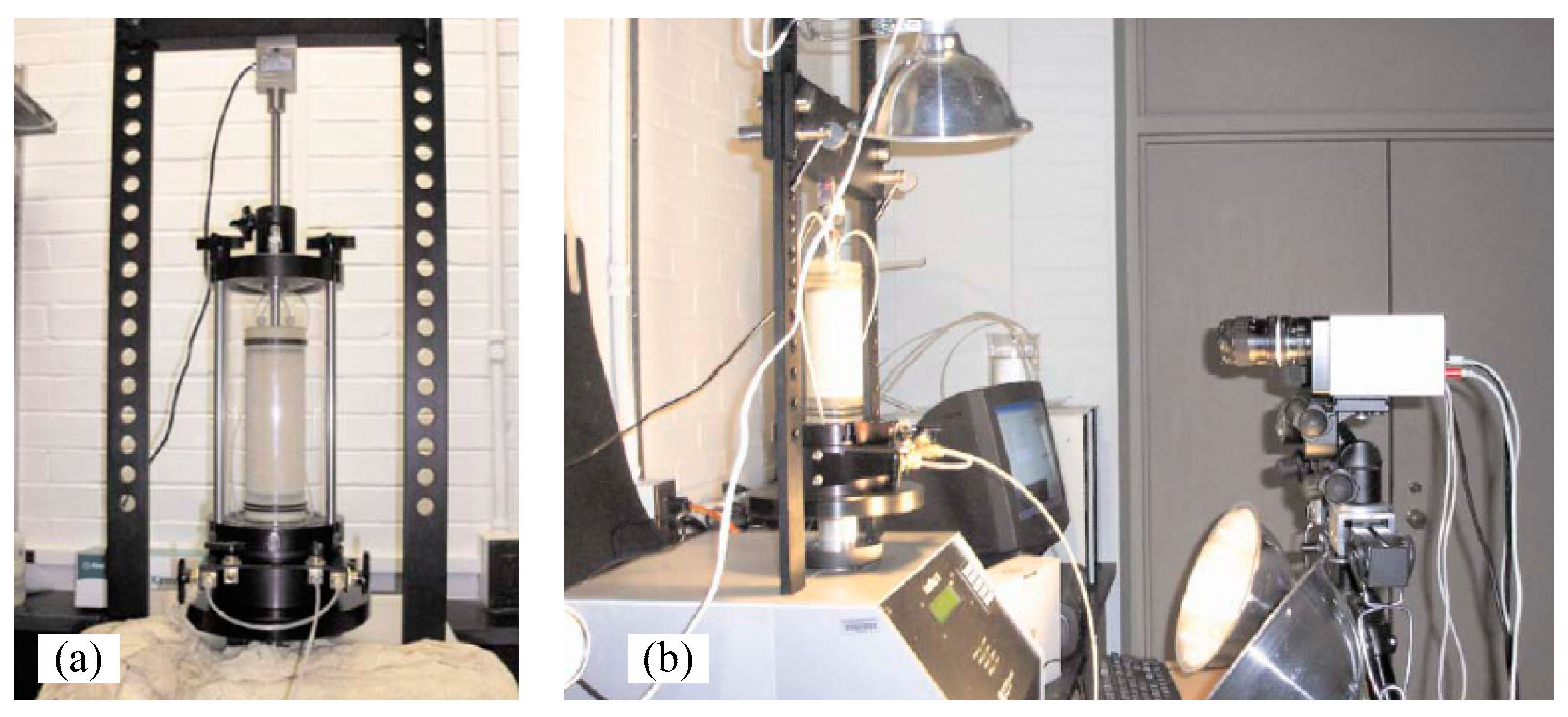
2.1. Triaxial Test

The triaxial test and 3D digital imaging systems used to measure both global and local deformations are shown in Figure 1. Further description of this system, its calibration, and the experimental methodology used to quantify both global and local deformations can be found in [1,2,3,4]. The triaxial experimental setting included a load cell controlled at a constant strain rate of 0.2%/min by a Geocomp triaxial automated system [33] and a transducer used to record the global loads and displacements during the experiments. To avoid optical distortion that may disturb interpretation of the digital images, an isotropic compression on the three specimens was set up using a vacuum pump instead of the plexiglass cell.

The imaging system consisted of two digital cameras installed in front of the sand specimen. The cameras produce stereo-digital images at every 0.05% axial strain. Digital images were acquired during increasing axial strain from 0% to approximately 12%, corresponding to boundary displacement fields from the undeformed configuration to peak and critical states. The overall coverage of the specimen’s boundary by the 3D-DIC produced displacement fields on approximately one-fourth of its cylindrical surface (85 degrees cone angle as measured from a horizontal cross-section of the specimen).

The characteristics of the three experimental tests used in this study are summarized in

Table 1. Summary of experimental tests used in this study [1].

Case	Test Name	Height (mm)	Diameter (mm)	Initial Density (kg/m3)	Relative Density (%)	Confinement (kPa)	Sample Preparation
Dense	120904c	159.67	71.11	1713.13	91.83	40	Vibratory compaction
Loose	121304b	158.17	70.86	1588.84	46.39	40	Dry pluviation
Half-densehalf-loose layered	120704c	157.67	70.88	1648.06 (avg.)	68.90 (avg.)	40	Vibratory compaction (two layers)
	Upper	78.17	70.68	1549.61	30.54	40
	Lower	79.50	71.27	1764.17	98.87	40

. The dense sand specimen (test 120904c) was constructed with three compacting layers to achieve a relative density of 91.83%, while the loose sand specimen (test 121304b) was prepared to reach a relative density of 46.39% by a dry pluviation method. Both test specimens were assumed to be homogeneous by design for this work. The half-dense half-loose layered sand specimen (test 120704c) consisted of two distinct compacting layers, which can be assumed as a heterogeneous configuration by design. The lower and upper segments were constructed to show a distinctive contrast with their relative densities of 98.87% and 30.54%, respectively, with the mid-height of the specimen as its boundary.

2.2. Digital Image Correlation (3D-DIC)

The digital images captured on the specimen’s boundary at each deformation stage during the experiments were utilized for quantifying the local displacement fields and volumetric changes [1]. Figure 2 illustrates an example of the deforming sequence of the dense sand specimen (test 120904c). These digital images were acquired at the 0.2%, 3.6%, 7%, and 12% axial strain levels, which represent the state of the specimen corresponding to the elastic, peak stress, softening, and critical state deformation phases, respectively.

The VIC-3D software [35] was introduced to solve the conversion process of the digital images at the specimen boundary into the vertical, horizontal, and out-of-plane incremental displacement fields. The discrete displacement fields for individual strain intervals were calculated in an incremental form to produce a full deformation sequence from 0% to 12% of axial strain. The computation process to estimate the cumulative displacement fields is described in detail in Medina-Cetina et al. [1].

Figure 3 and Figure 4 illustrate the states of deformation at 0.2% and 12.0% of axial strain corresponding to the elastic and critical states, respectively, for the three sand specimens of interest (i.e., dense, loose, and half-dense half-loose layered). Each one of these figures includes a reference picture (left) and its three components of the cumulative displacement fields (vertical, radial, and tangential components).

At the elastic state (Figure 3, 0.2% of axial strain), just after the specimens’ axial compression starts, it is observed a relatively uniform distribution of the vertical displacement fields along the vertical direction of the specimen, which are consistent with the displacement induced at the bottom of the specimen to load it; the radial displacement fields show a slight inward and outward displacement reflecting an initial adjustment of the specimen to the load imposed; the tangential component of the displacement fields show a slight rotation of the specimen, also consistent with the initial accommodation of the specimens to the initial loading.

At critical state (Figure 4, 12.0% of axial strain), the vertical displacement component for the dense and loose specimens show an initial uniform distribution, which becomes non-uniform at later stages of deformation, while the half-dense half-loose specimen shows a rigid type of displacement at the bottom compared with its upper section; the radial displacement components show a similar initial uniform behavior for the dense and loose specimens that become non-uniform at later stages of deformation, while the half-dense half-loose specimen shows limited radial displacement compared with its upper segment; finally, the tangential components show evidence of shear banding for the dense and loose specimens showing a non-uniform behavior, while the half-dense half-loose specimen shows a twist between the lower and upper segments, with the lower segment twisting to the right while the upper segment twisting to the left. The upper segment of the half-dense half-loose specimen shows a relatively significant deformation compared to its lower segment, which means that the specimen’s global deformation is mainly concentrated on the upper segment.

To compare the boundary response of an axisymmetric numerical model with the boundary observations produced by the 3D-DIC, the vertical and radial displacement field components are reduced from a 3D to a 1D representation, producing two vertical profiles. These are estimated as the averaged vertical and averaged radial displacements, respectively as described in Medina-Cetina et al. [1]. To illustrate the boundary vertical and radial displacements of the specimen using a 1D vertical profile representation, Figure 5 shows the compression deformation sequence for the dense sand specimen (120904c). From this figure, it is observed that the radial displacement fields mainly represent the bulging effect of the specimen, which shows higher displacement values around the mid-height of the sample. Notice that the vertical displacements at the bottom of the specimen corresponding to the global displacement that follows the strain rate during shearing. Similar profiles were estimated for the loose and the half-dense half-loose specimens.

3. Finite Element Modeling of Triaxial Tests

This section presents a proposed finite element modeling approach for simulating the triaxial compression tests described above and the soil parameter estimation process based on their corresponding experimental data.

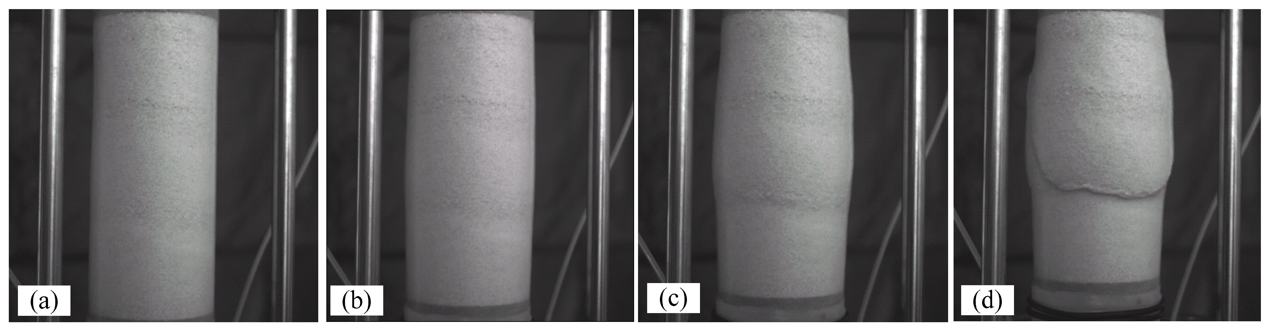
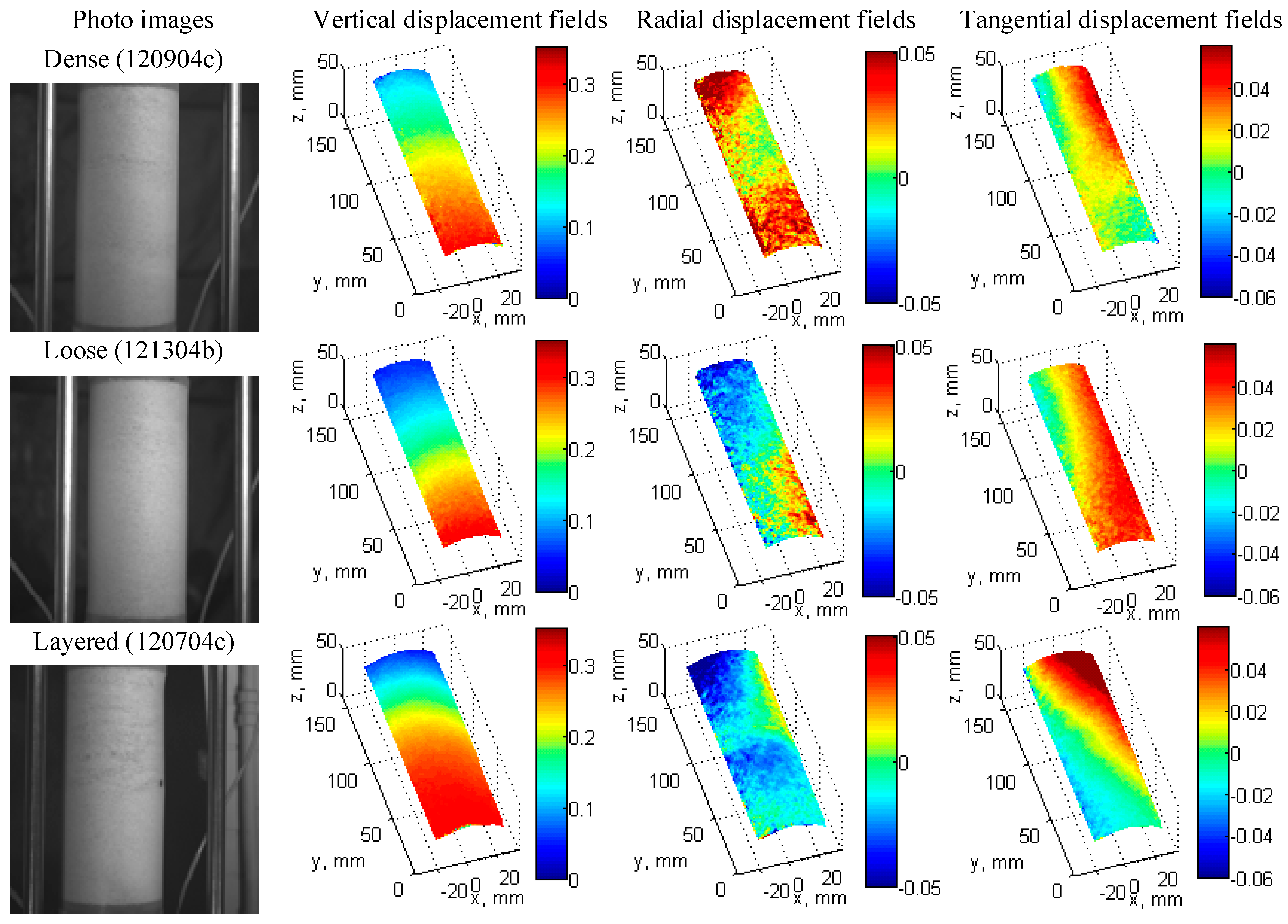
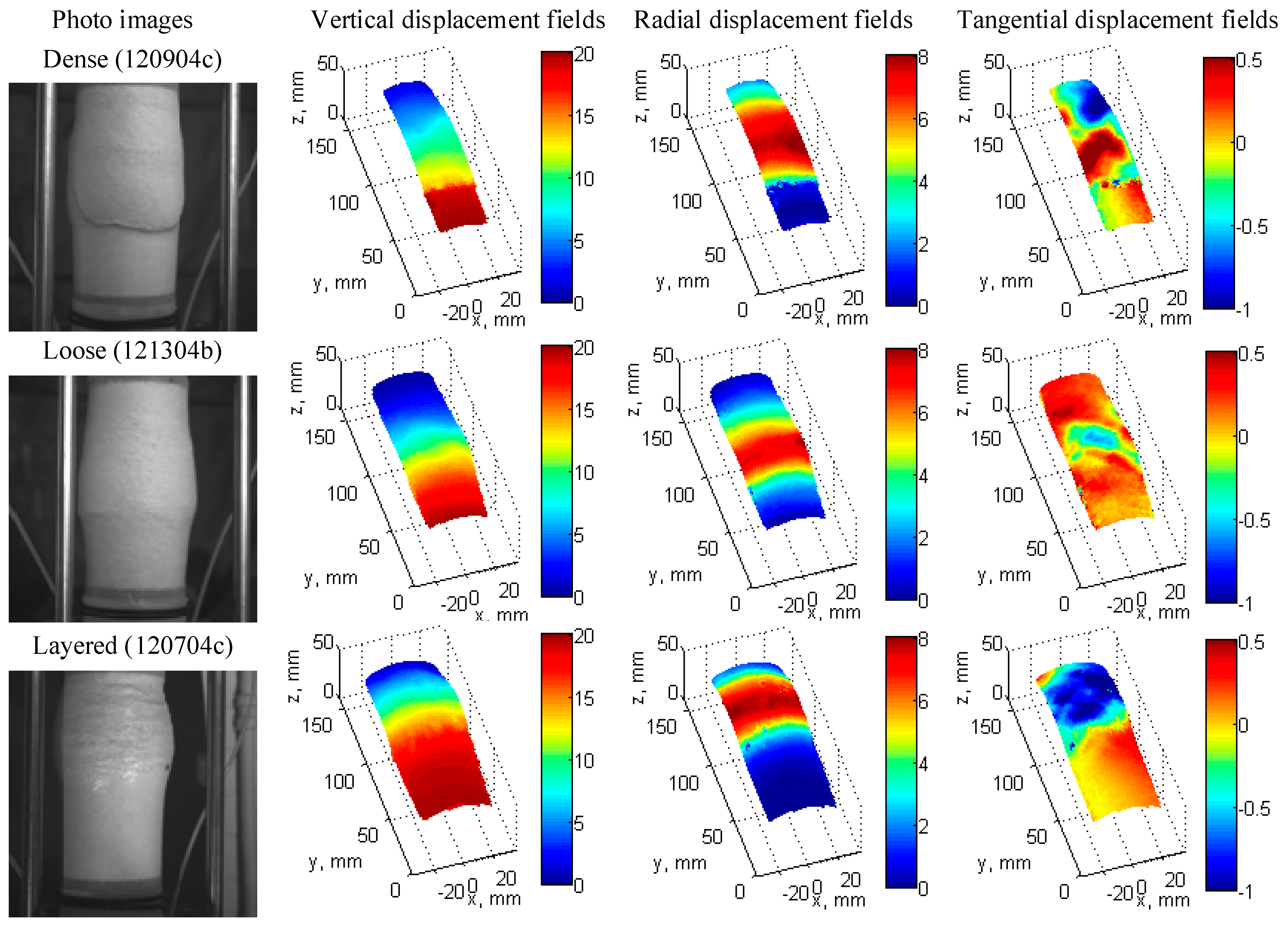
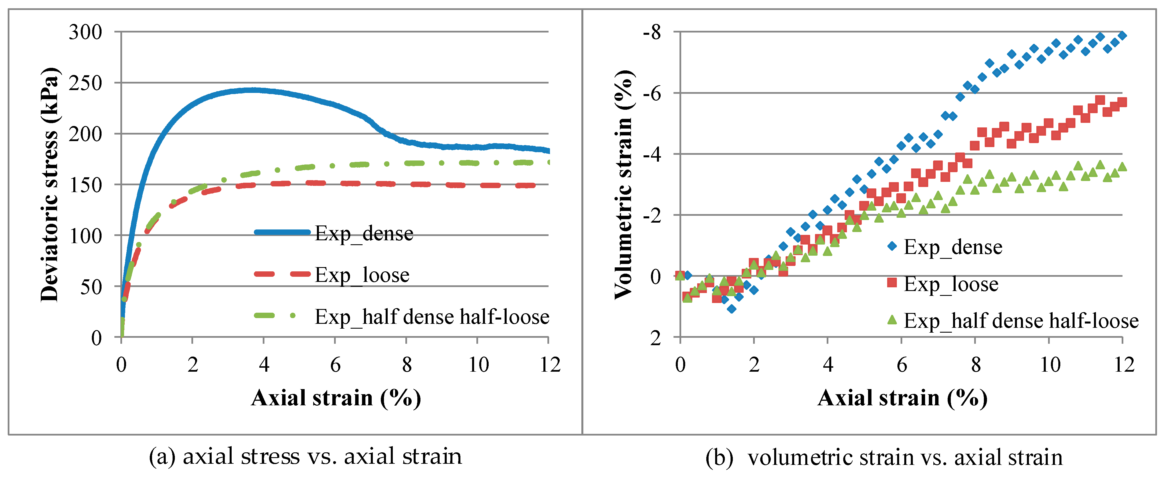
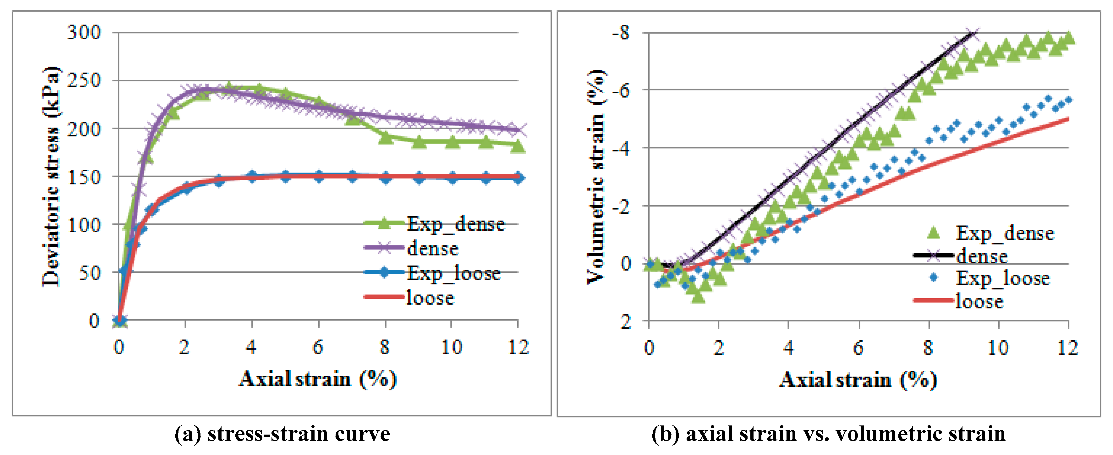
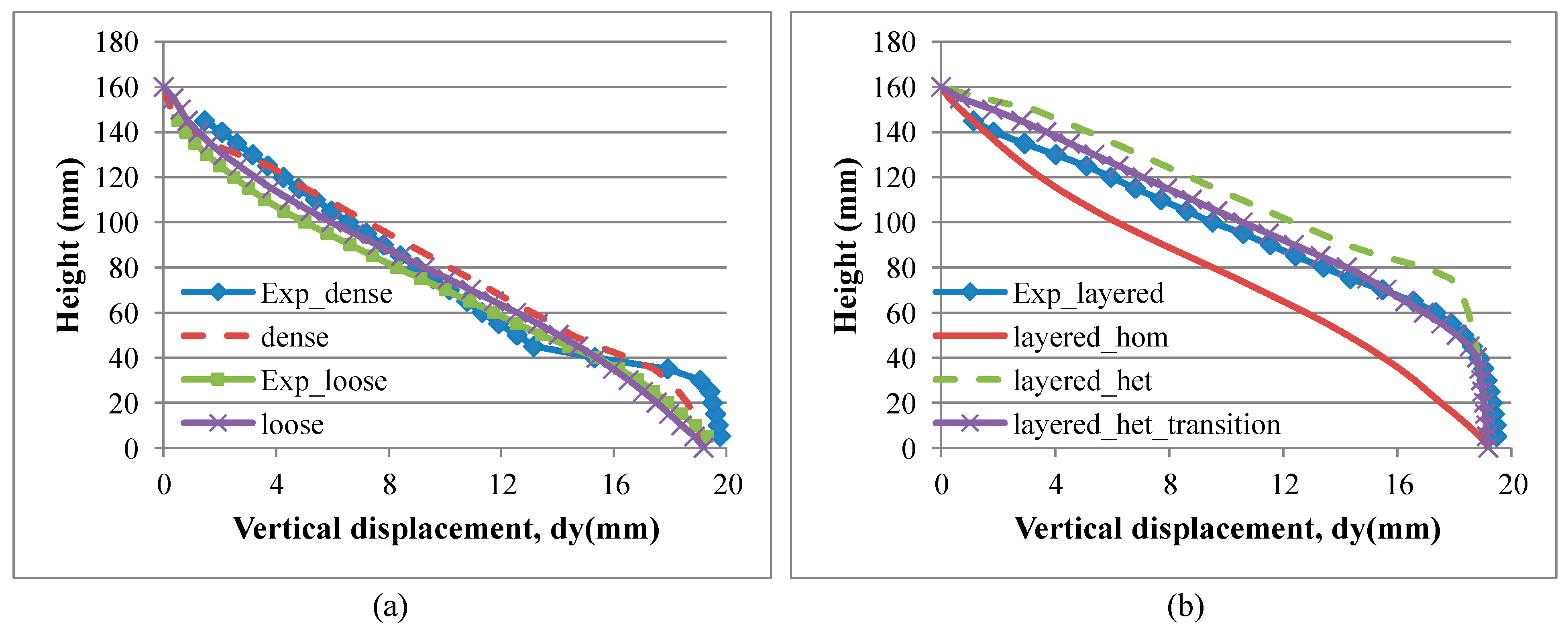
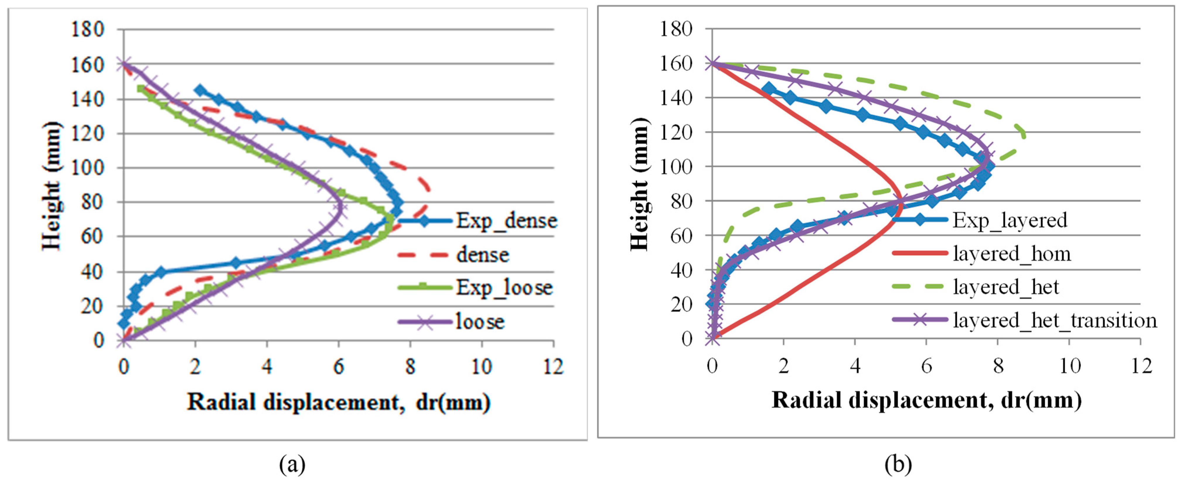
3.1. Experimental Behavior of Dense, Loose, and Half-Dense Half-Loose Specimens

The global stress-strain behavior was analyzed because the triaxial compression tests were examined for the dense, loose, and half-dense half-loose layered specimens (with different relative densities). A comparison of the behavior of the three specimens is shown in Figure 6, introducing the axial stress vs. axial strain and the volumetric strain vs. axial strain curves.

The axial stress vs. axial strain response of the dense and loose specimens shows a typical mechanical behavior with hardening and softening for the dense specimen and hardening only for the loose specimen (Figure 6a). The mechanical response of the half-dense half-loose specimen shows a typical behavior of a loose sand specimen, which means that its ‘global’ behavior is somehow controlled by the half-loose segment of the specimen and that the averaged material parameters of the two specimen’s layers would overestimate the actual specimen’s behavior.

Volumetric strains of all three specimens show a dilatant behavior (Figure 6b). Relative densities of loose and half-dense half-loose specimens oscillate between 46.39% and 68.90%, respectively. Note that the relative density of the half-dense half-loose specimen is a weighted average value that was computed from the total volume of the specimen relative to the height of each layer. Granular materials with 15% to 50% of relative density can be defined as loose, granular materials with 50% to 70% of relative density can be defined as medium dense, while granular materials with relative density higher than 70% can be defined as dense material [36]. However, some experimental data of sands with relative density between 42% and 47% show dilation in global volumetric strain behavior [37].

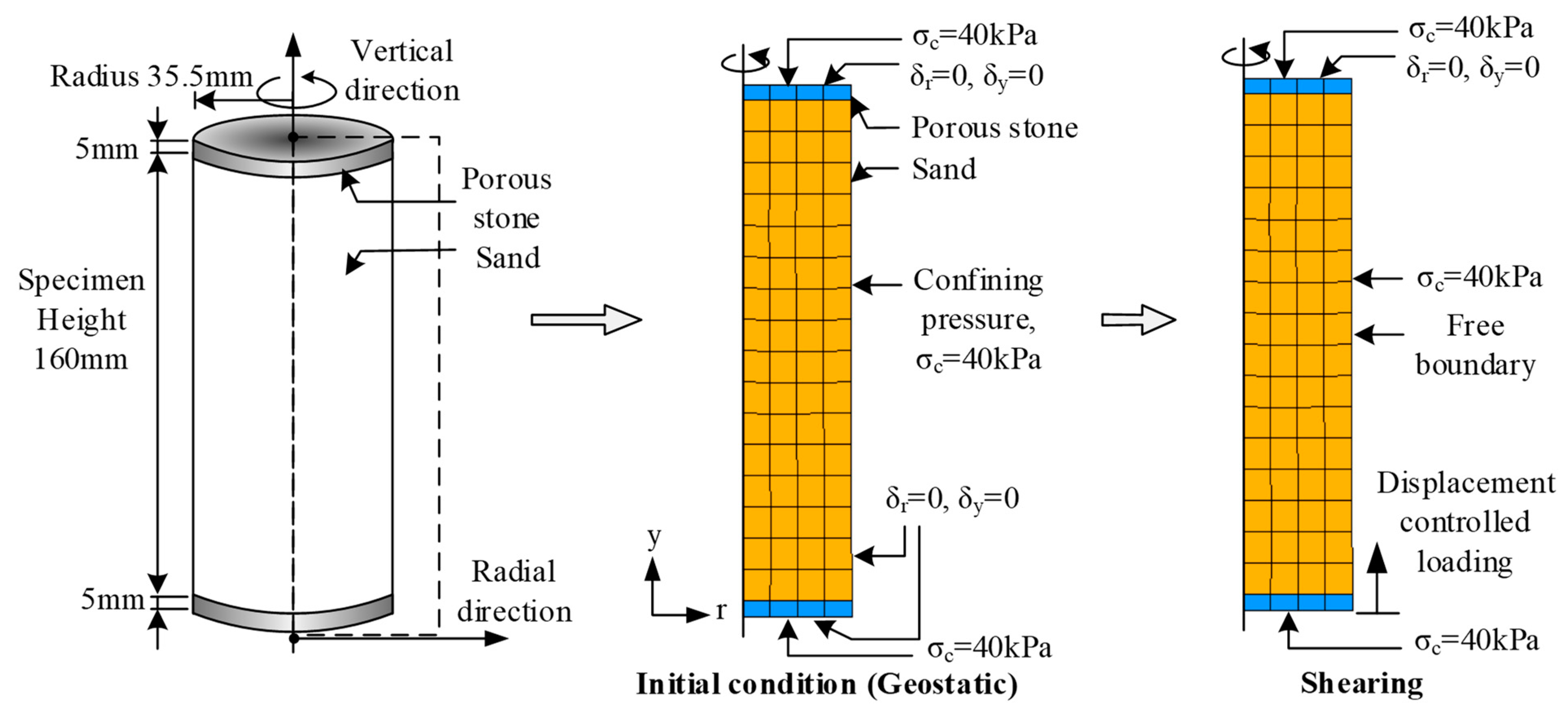
3.2. Finite Element Model

An axisymmetric finite element model was formulated to simulate the triaxial compression of the dense, loose, and half-dense half-loose specimens (Figure 7). The commercial finite element program ABAQUS [31] was used to simulate the specimen experimental response. An elasto-plastic constitutive model based on Mohr–Coulomb was considered. The constitutive model and parameter estimation chosen to best describe the experimental behavior of the specimens are discussed in a later section.

The initial stress condition was specified by adopting the ‘geostatic’ option available in ABAQUS to calculate the stress, which is in equilibrium with the external loading and boundary conditions. That means that the displacements occurring in the geostatic step should be near zero or negligible for the equilibrium condition, and at the same time, the effect of the vacuum consolidation was reproduced by applying a surface-distributed loading boundary condition of 40 kPa at the top, bottom, and lateral surfaces of the model.

The compression load observed during the automated triaxial tests was also reproduced in the FEM model (i.e., 0.2% of axial strain/min), which was introduced as a displacement-controlled loading at the bottom of the model. At the same time, lateral boundary displacements were allowed while the isotropic confining pressure was maintained during the compression loading of the specimen.

The initial boundary conditions of the sand specimens were defined by their observed initial geometry (before the start of the compression load) and included in the formulation of the model. Figure 8 shows the vertical profiles of each of the three specimens analyzed in this paper. This Figure shows the specimen’s radius oscillating between 35.2 mm and 36.6 mm among the three specimens (notice that there are two figures at different scales showing the same variation of the specimen’s radius).

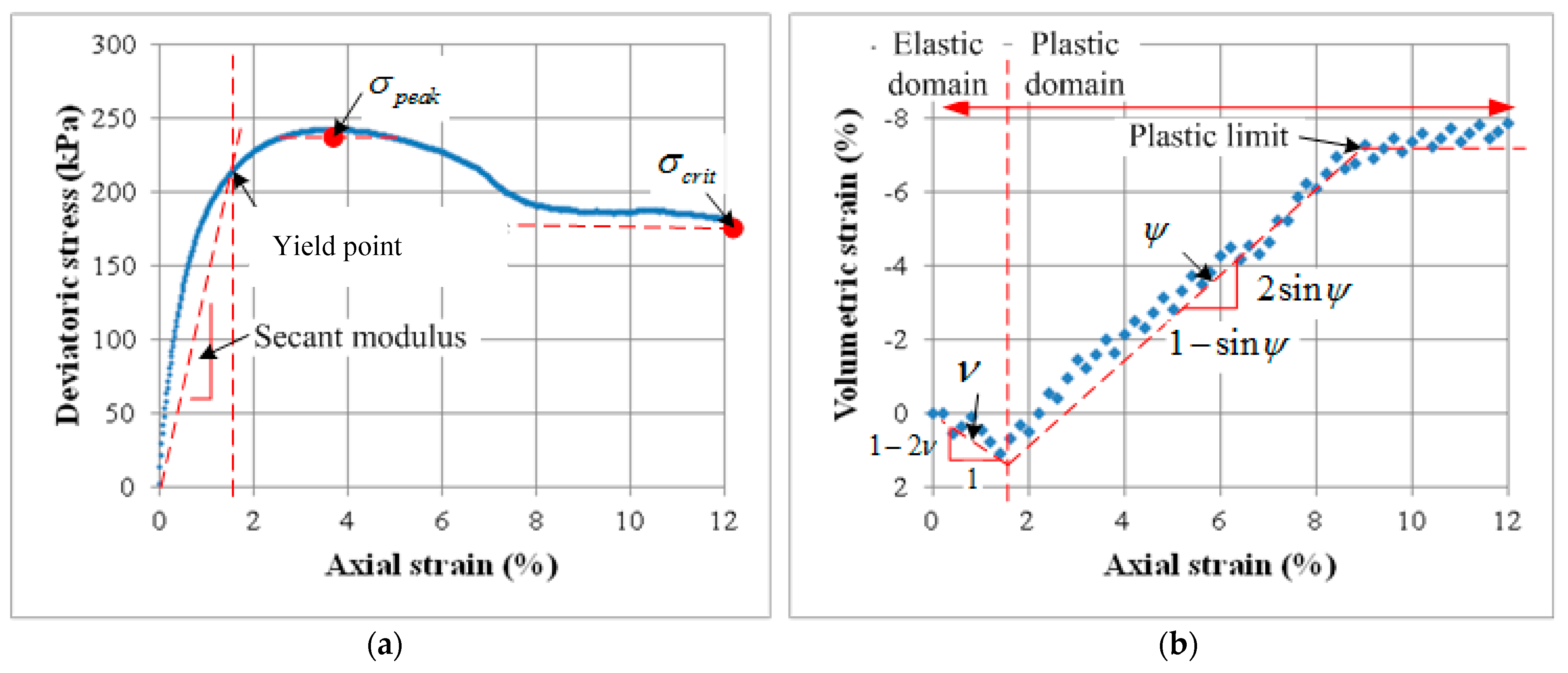
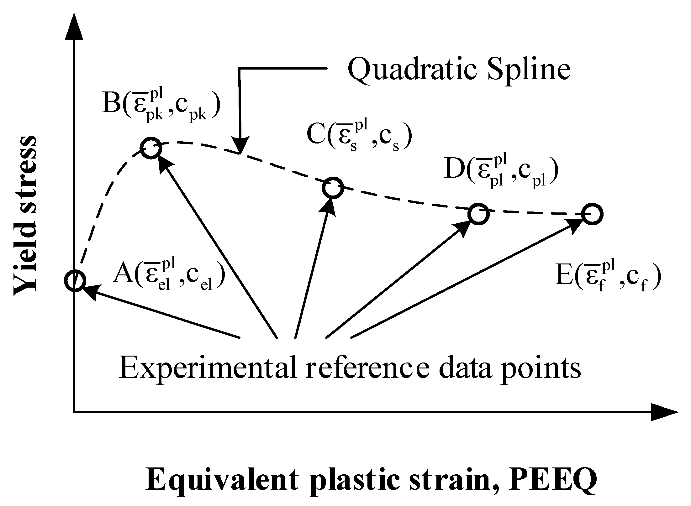
3.3. Proposed Elasto-Plastic Constitutive Model and Parameters

To simulate the hardening and softening behavior of the three sand specimens, an elasto-plastic constitutive model based on the Mohr–Coulomb model formulation available in ABAQUS was considered suitable to reproduce the given sand specimens. The classical Mohr–Coulomb plasticity model defines the yield surface as a function of cohesion and internal friction angle. It requires a relatively simple number of variables among plasticity constitutive models, and for this reason, it is widely used in computational analysis to solve geoengineering problems. The elastic phase was considered linear elastic as defined by Hooke’s law.

The interpretation of the triaxial results makes it possible to represent the dilative behavior of the sand by using an elasto-plastic model such as Mohr–Coulomb. The elastic and plastic parameters deduced from the experimental database were [1] as follows: Poisson’s ratio, Young’s modulus, dilation angle, and axial strains at the yield point and plastic limit, as shown in Figure 9. These parameters were determined from the triaxial test readings based on definitions by Gay et al. [38]. The internal friction angle was determined by drawing a best-fit straight-line tangent to Mohr’s circle diagram at the peak strength, assuming zero cohesion [1,39], as it is a standard procedure to elicit the friction angle from standard triaxial (global) observations.

The determination of hardening and softening parameters was inspired by a simple hardening rule consisting of segment zones, proposed by Potts and Zdravkovic [40]. This allowed for the variation of the accumulated plastic strains observed in the triaxial experiments. ABAQUS allows a introduction of a hardening and softening curve that consists of the equivalent plastic strain (PEEQ or ${\overline{\mathsf{\epsilon }}}^{\mathrm{pl}}$) and yield stress (cohesion for the Mohr–Coulomb model). The relation between the equivalent plastic strain and yield stress is defined as a smooth curve using a quadratic spline interpolation to the stress-strain experimental curves. As shown in Figure 10, this curve can be divided into five reference data points representing the elastic limit (A), peak state (B), softening state (C), the onset of the critical state (D), and the final critical state (E). Then, the values at these points suggest strain-hardening and softening parameters for each segment zone. Further details about the implementation of this methodology can be found in Song [39].

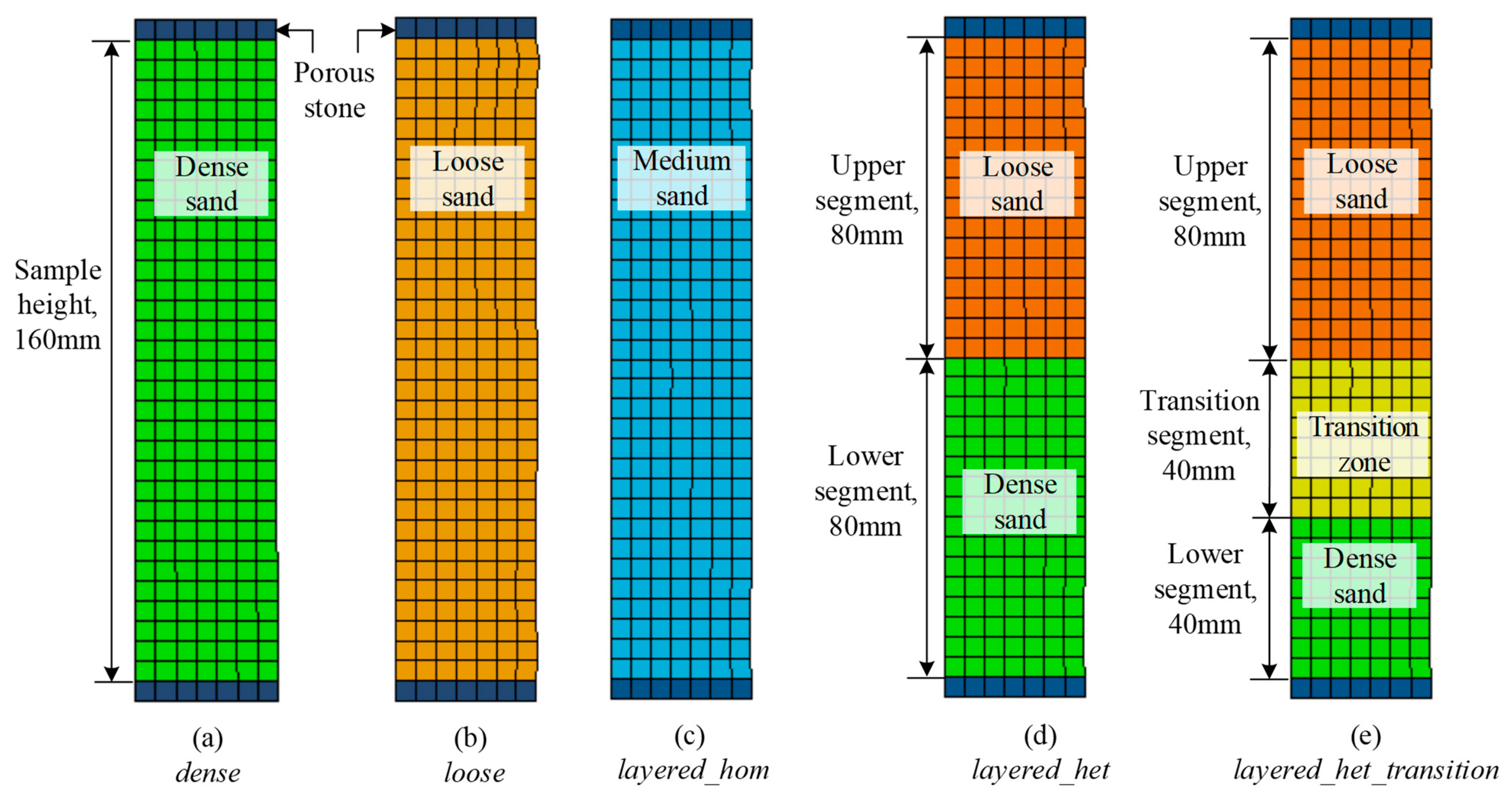
3.4. Analysis Cases of Homogeneous and Heterogeneous Specimens

Five models were drafted to reproduce the mechanical behavior of the three sand experiments considered in this paper (i.e., dense, loose, and half-loose half-dense). A first set of models assumed the following three given experiments as homogeneous specimens: The dense experiment (dense model, Figure 11a), the loose experiment (loose model, Figure 11b), and the half-loose half-dense specimen (layered_hom, Figure 11c). A second set of models assumed the half-loose half-dense experiment as a heterogeneous specimen (layered_het, Figure 11d; layered_het_transition, Figure 11e). Figure 11d is composed of two layers, each 80 mm high, to have the same configuration as the test specimen, while Figure 11e is composed of a simplified transition zone with a height of 40 mm between the upper and lower segments, inferred based on the vertical displacement analysis of the experimental results. All input parameters to run these models were based on the experimental results using observations of the specimens’ global behavior (Figure 6).

The summary of the experimental material properties for the dense, loose, and the half-dense half-loose specimens are presented in

Table 2. Summary of material properties for dense, loose, and layered specimens.

Case	Configuration	Unit Weight (kN/m3)	Young’s Modulus (kPa)	Poisson’s Ratio	Friction Angle (deg)	Dilation Angle (deg)
Dense	Dense	20	21,559	0.44	43.09	22.78
Loose	Loose	20	15,818	0.25	32.86	14.48
Layered_hom	Medium	20	18,164	0.20	32.12	11.97
Layered_het	Upper loose	20	15,818	0.25	32.86	14.48
	Lower dense	20	21,559	0.44	43.09	22.78
Layered_het_transition	Upper loose	20	15,818	0.25	32.86	14.48
	Transition zone	20	20,361	0.37	36.86	18.19
	Lower dense	20	21,559	0.44	43.09	22.78
Porous stone	-	20	1,000,000	0.20	-	-

. Notice that for the half-dense half-loose specimen (layered_het, Figure 11d), the lower dense segment is assigned properties corresponding to the dense specimen, and the upper loose segment is assigned properties of the loose material. The model that includes the transition zone (layered_het_transition, Figure 11e) follows a similar approach to assign the model properties to the dense and loose segments and to assign values to parameters of the ‘transition zone’, these were computed by averaging the specimens’ dense and loose stress-strain curves and then estimating the model parameters as if this was a new experimental stress-strain curve.

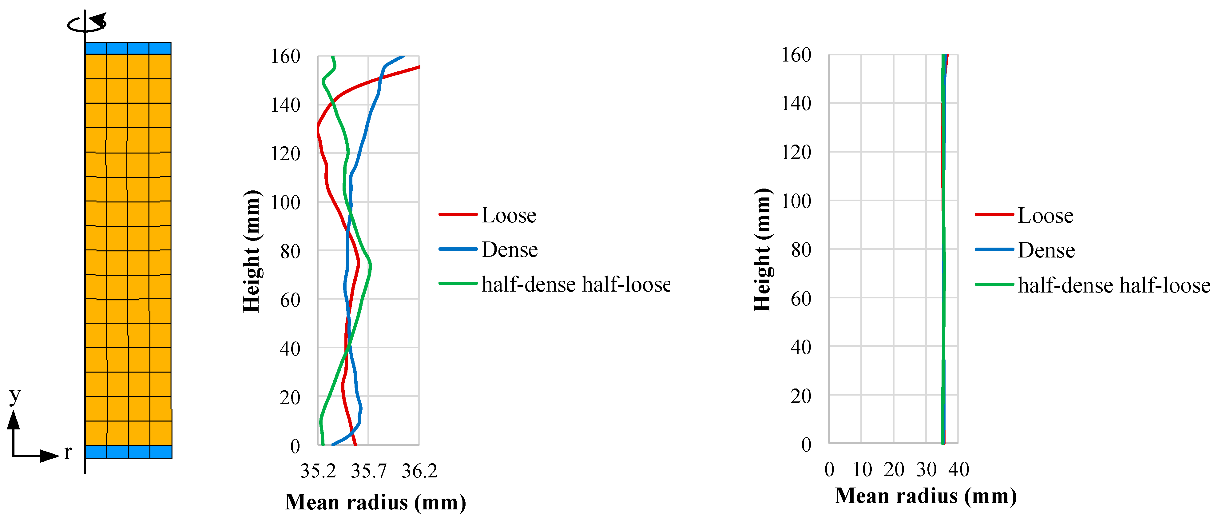
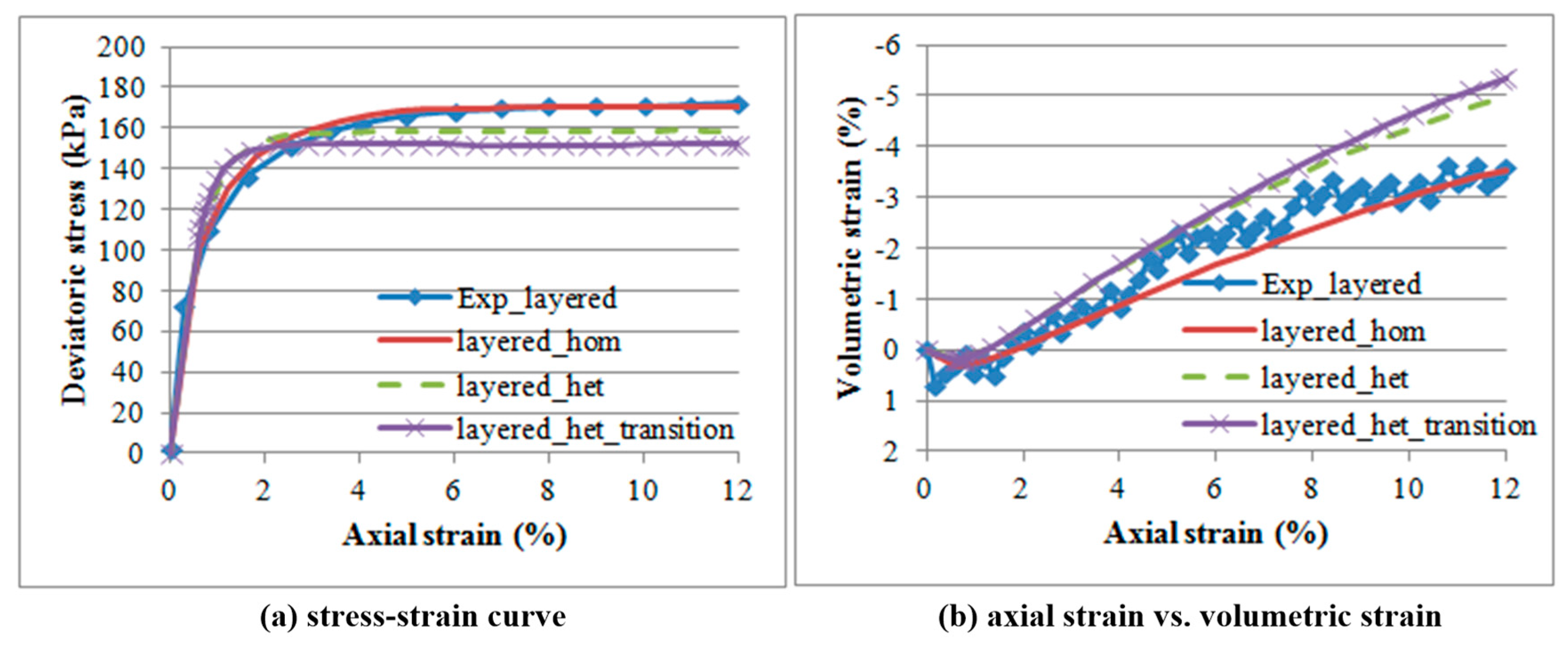
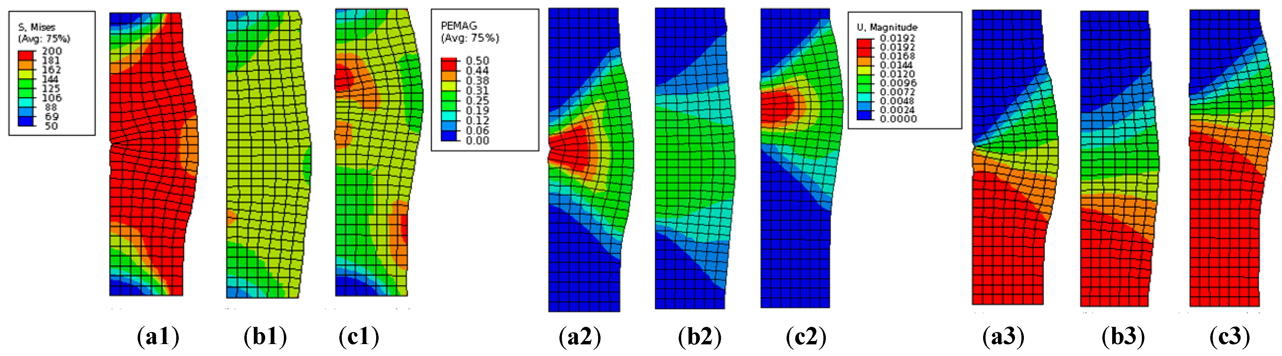
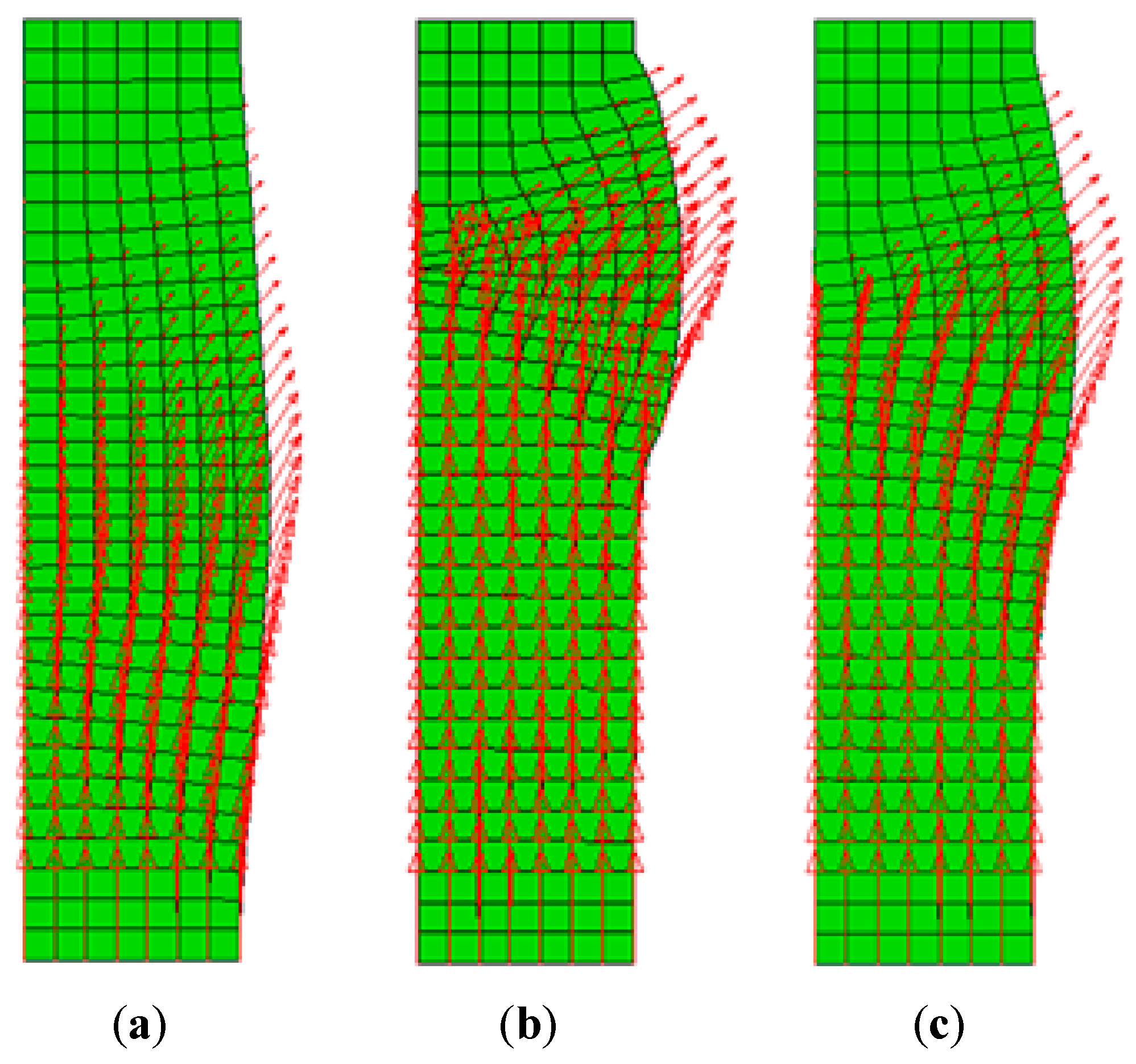
4. Results and Discussion

The three given triaxial compression experimental tests considered in this paper (dense, loose, and half-dense half-loose specimens) were compared with the finite element models presented in the previous section.

Figure 12 compares model predictions with the experimental results for the dense (Exp_dense curve) and the loose (Exp_loose curve) specimens, both assuming a homogeneous composition. Model predictions show a good agreement with the experimental tests in terms of their global stress-strain response. Figure 13 compares model predictions with the experimental results for the half-dense half-loose specimen (Exp_layered curve) for the three model configurations (layered_hom, layered_het, layered_het_transition). Model predictions show a good agreement with the experimental tests in terms of stress-strain behavior, with the ‘layered_hom’ model showing the best fit to the experimental response, while the two heterogeneous models show from 10 to 20 kPa deviation at the critical state.

Regarding the axial strain vs. volumetric strain, the best agreement is for the cases (loose curve, layered_hom) with the homogeneous material model and a bulging failure mode. In the case of dense (dense curve), in which a failure mode by apparent shear is observed, and the heterogeneous material (layered_het and layered_het_transition), a slight deviation is observed about after 8% of axial strain, which coincides with the starting of the critical state.

A comparative analysis showing local deformations between model predictions and experimental observations are presented in Figure 14 and Figure 15, following the same approach as described above when comparing axial strain vs. axial stress and axial strain vs. volumetric strain, respectively. This analysis is set at 12% of axial strain, which approximately corresponds to the critical state.

Here the possibility of simulating the local observations of displacement fields, which is easily overlooked in the triaxial point sensor readings but is captured in the experimental database used in this study, is demonstrated through the finite element model. In addition, it is provided that the local effect, where the failure mode is clearly identified in a form of such as a location of a shear band and the maximum deformation radius by bulging, can be improved by the calibration process of the finite element model.

Figure 14a shows predictions of vertical displacements along the boundary of the specimens for the dense and loose specimens, showing good agreement with the corresponding experimental observations (vertical profiles of averaged vertical displacements observed at the same height of the specimen are estimated via digital image analysis). Figure 14b shows predictions of vertical displacement along the boundary of the specimens for the half-dense half-loose model configurations, where it is observed that the heterogenous models (layered_het and layered_het_transition) show good agreement with the experimental observations, while the homogeneous model (layered_hom) shows a significant deviation from the experimental behavior. From the heterogeneous models, the best fit for the experimental observations is the layered model with the transition zone (layered_het_transition).

Figure 15a shows predictions of radial displacement along the boundary of the dense and loose specimens, showing an overall agreement with experimental observations but some local deviations (vertical profiles of averaged radial displacements observed at the same height of the specimen are estimated via digital image analysis), both showing a relative sub-estimation of the maximum radial displacements and the dense model with a relative sub-estimation of the radial displacement and the bottom of the specimen. Figure 15b shows that the layered homogeneous model (layered_hom) is not in agreement with the experimental observations, showing an expected symmetric behavior due to its single and homogeneous layer composition; the other two layered models (layered_het and layered_het_transition) show a much better agreement with experimental observations, with the model including the transition zone showing the best fit to the experimental observations, which is an indication that there is a stiffness reduction on the upper segment of the dense layer (bottom layer), which is consistent with experimental compaction methods during sample preparation.

Figure 16 presents stress (left, denoted by number 1 following the alphabet), plastic strain (middle, denoted by number 2 following the alphabet), and total displacement (right, denoted by number 3 following the alphabet) contours of three model cases, i.e., dense, loose and layered_het_transition at 12% of axial strain. The shear banding and failure patterns were already well-tracked by DIC, but there were limitations to be inferred from boundary displacement fields. These contour plots provide insight into the stress and plastic strain distributions within the model by showing its cross-section, which helps to better understand the failure mechanisms associated with each specimen.

Figure 17 presents total displacement vectors on a deformed mesh of the half-loose half-dense specimen (i.e., layered models) as follows: the homogeneous model (layered_hom, Figure 17a) deformed into a barrel shape similar to that observed with the loose specimen; the deformation features observed in the heterogeneous models (layered _het, Figure 17b; layered_het_transition, Figure 17c), confirmed that they occur mainly in the upper loose section, which is known as the weaker segment of the specimen.

5. Conclusions

This paper introduces a method for constructing a predictive model that reproduces both the global and the local non-homogeneous response of a triaxial compression test of different sand specimens. A series of stereo-photo images taken during a compression test generated 3D displacement fields on the sample boundary by the use of the digital image correlation (DIC) technique. This showed that DIC can be effectively used to track the evolution of the displacement fields. By leveraging the advantage of the boundary displacement fields obtained by DIC compared to the traditional global measurements (i.e., axial stress vs. axial strain and volumetric strain vs. axial strain), the material constitutive model was calibrated, showing its suitability to capture both global and local deformation effects.

A comparative analysis of model predictions and experimental observations was conducted on the following three distinct triaxial sand specimens: dense, loose, and half-dense and half-loose. The modeling approach was based on the use of an axisymmetric finite element model, using an adaptation of the ABAQUS Mohr–Coulomb material implementation. Based on the use of boundary information of the kinematics generated by a 3D digital image correlation analysis, it was possible to reproduce the elasto-plastic specimens’ behavior, including hardening and softening. All model predictions were based on parameters generated from the triaxial experiments. Two sets of models were formulated to reproduce the dense, loose, and half-dense and half-loose specimens. First, the dense and loose specimens (dense and loose models, respectively) and the half-dense half-loose specimen (layered_hom) assumed a homogeneous composition. Second, the half-dense half-loose specimen (layered_het, layered_het_transition) assumed a heterogeneous composition.

Results of both analyses showed that the best predictions for axial strain vs. stress and for axial strain vs. volumetric strain corresponded to the use of the homogeneous models, meaning that the traditional assumption made to capture the ‘global’ triaxial response based on the use of one loading cell, one displacement transducer, and one volumetric transducer, as configured on standard triaxial devices, is consistent with the selection of the proposed models’ material (i.e., modified ABAQUS Mohr–Coulomb implementation to account for softening and hardening). However, when comparing the model predictions with the experimental boundary displacements in the vertical and radial directions, there were observed significant deviations when assuming a homogeneous specimen. This called for the need to introduce the use of heterogeneous models that can account for a more realistic density variation, as illustrated by the sequence of the three models reproducing the half-loose half-dense specimen. Moreover, even in the use of the heterogeneous model, the result of introducing the transition zone between the loose and dense segments showed a better deformation response than the experimental configuration of the half-dense half-loose specimen. This suggests that it is necessary to consider the interaction between two layers with a large relative density difference.

The model parameters used in this work were generated directly from the experimental configuration of the specimens. This approach sets the basis as well for a more comprehensive calibration process, as discussed in the following paper, where model parameters are defined as spatially distributed variables within the sand specimen and where the experimental observations cover a significant segment of the specimens’ surface (as opposed to what is presented in this work, where the boundary observations are averaged along the vertical direction).

References

1. Medina-Cetina, Z.; Song, A.; Zhu, Y.; Pineda-Contreras, A.R.; Rechenmacher, A. Global and Local Deformation Effects of Dry Vacuum-Consolidated Triaxial Compression Tests on Sand Specimens: Making a Database Available for the Calibration and Development of Forward Models. Materials 2022, 15, 1528. [Google Scholar] [CrossRef] [PubMed]
2. Zhu, Y.; Medina-Cetina, Z.; Pineda-Contreras, A.R. Spatio-Temporal Statistical Characterization of Boundary Kinematic Phenomena of Triaxial Sand Specimens. Materials 2022, 15, 2189. [Google Scholar] [CrossRef] [PubMed]
3. Zhu, Y.; Medina-Cetina, Z. Assessment of Spatio-Temporal Kinematic Phenomena Observed along the Boundary of Triaxial Sand Specimens. Appl. Sci. 2022, 12, 8091. [Google Scholar] [CrossRef]
4. Zhu, Y.; Medina-Cetina, Z. Statistical Characterization of Boundary Kinematics Observed on a Series of Triaxial Sand Specimens. Appl. Sci. 2022, 12, 11413. [Google Scholar] [CrossRef]
5. Duncan, J.M. The role of advanced constitutive relations in practical applications. In Proceedings of the 13th International Conference Soil Mechanics and Foundation Engineering, New Delhi, India, 5–10 January 1994; Volume 5, pp. 31–48. [Google Scholar]
6. Potts, D.M. Numerical analysis: A virtual dream or practical reality? Géotechnique 2003, 53, 535–573. [Google Scholar] [CrossRef]
7. Brinkgreve, R.B.J. Selection of Soil Models and Parameters for Geotechnical Engineering Application: Soil Constitutive Models: Evaluation, Selection, and Calibration. Geotech. Spec. Publ. 2005, 128, 69–98. [Google Scholar] [CrossRef]
8. Lade, P.; Kim, M. Single hardening constitutive model for frictional materials III. Comparisons with experimental data. Comput. Geotech. 1988, 6, 31–47. [Google Scholar] [CrossRef]
9. Boldyrev, G.G.; Idrisov, I.K.; Valeev, D.N. Determination of parameters for soil models. Soil Mech. Found. Eng. 2006, 43, 101–108. [Google Scholar] [CrossRef]
10. Lade, P.V. Overview of constitutive models for soils. In Soil Constitutive Models: Evaluation, Selection, and Calibration; Yamamuro, J.A., Kaliakin, V.N., Eds.; ASCE Geotechnical Special Publication No. 128; ASCE: Reston, VA, USA, 2005; pp. 1–34. [Google Scholar] [CrossRef]
11. Sutton, M.; Wolters, W.; Peters, W.; Ranson, W.; McNeill, S. Determination of displacements using an improved digital correlation method. Image Vis. Comput. 1983, 1, 133–139. [Google Scholar] [CrossRef]
12. Sutton, M.A.; McNeill, S.R.; Helm, J.D.; Chao, Y.J. Advances in Two-Dimensional and Three-Dimensional Computer Vision. Photomech. Top. Appl. Phys. 2000, 77, 323–372. [Google Scholar] [CrossRef]
13. Sutton, M.; Yan, J.; Tiwari, V.; Schreier, H.; Orteu, J. The effect of out-of-plane motion on 2D and 3D digital image correlation measurements. Opt. Lasers Eng. 2008, 46, 746–757. [Google Scholar] [CrossRef] [Green Version]
14. Schreier, H.; Orteu, J.-J.; Sutton, M.A. Image Correlation for Shape, Motion and Deformation Measurements; Springer Science & Business Media: Boston, MA, USA, 2009. [Google Scholar] [CrossRef]
15. Hall, S.; Bornert, M.; Desrues, J.; Pannier, Y.; Lenoir, N.; Viggiani, G.; Bésuelle, P. Discrete and continuum analysis of localised deformation in sand using X-ray μCT and volumetric digital image correlation. Géotechnique 2010, 60, 315–322. [Google Scholar] [CrossRef]
16. Higo, Y.; Oka, F.; Sato, T.; Matsushima, Y.; Kimoto, S. Investigation of localized deformation in partially saturated sand under triaxial compression using microfocus X-ray CT with digital image correlation. Soils Found. 2013, 53, 181–198. [Google Scholar] [CrossRef] [Green Version]
17. Chaney, R.; Demars, K.; Macari, E.; Parker, J.; Costes, N. Measurement of Volume Changes in Triaxial Tests Using Digital Imaging Techniques. Geotech. Test. J. 1997, 20, 103. [Google Scholar] [CrossRef]
18. Suits, L.D.; Sheahan, T.; Rechenmacher, A.; Finno, R. Digital Image Correlation to Evaluate Shear Banding in Dilative Sands. Geotech. Test. J. 2004, 27, 10864. [Google Scholar] [CrossRef]
19. Rechenmacher, A.L.; Abedi, S.; Chupin, O.; Orlando, A.D. Characterization of mesoscale instabilities in localized granular shear using digital image correlation. Acta Geotech. 2011, 6, 205–217. [Google Scholar] [CrossRef] [Green Version]
20. Wang, P.; Sang, Y.; Shao, L.; Guo, X. Measurement of the deformation of sand in a plane strain compression experiment using incremental digital image correlation. Acta Geotech. 2018, 14, 547–557. [Google Scholar] [CrossRef]
21. Belheine, N.; Plassiard, J.-P.; Donzé, F.-V.; Darve, F.; Seridi, A. Numerical simulation of drained triaxial test using 3D discrete element modeling. Comput. Geotech. 2009, 36, 320–331. [Google Scholar] [CrossRef]
22. Cil, M.B.; Alshibli, K.A. 3D analysis of kinematic behavior of granular materials in triaxial testing using DEM with flexible membrane boundary. Acta Geotech. 2013, 9, 287–298. [Google Scholar] [CrossRef]
23. Lee, S.J.; Hashash, Y.M.; Nezami, E.G. Simulation of triaxial compression tests with polyhedral discrete elements. Comput. Geotech. 2012, 43, 92–100. [Google Scholar] [CrossRef]
24. Lu, Y.; Frost, D. Three-Dimensional DEM Modeling of Triaxial Compression of Sands. In Proceedings of the GeoShanghai International Conference 2010, Shanghai, China, 3–5 June 2010; pp. 220–226. [Google Scholar] [CrossRef]
25. Kawamoto, R.; Andò, E.; Viggiani, G.; Andrade, J.E. Level set discrete element method for three-dimensional computations with triaxial case study. J. Mech. Phys. Solids 2016, 91, 1–13. [Google Scholar] [CrossRef] [Green Version]
26. Kawamoto, R.; Andò, E.; Viggiani, G.; Andrade, J.E. All you need is shape: Predicting shear banding in sand with LS-DEM. J. Mech. Phys. Solids 2018, 111, 375–392. [Google Scholar] [CrossRef] [Green Version]
27. Kozicki, J.; Tejchman, J. Numerical simulations of triaxial test with sand using DEM. Arch. Hydro-Eng. Environ. Mech. 2009, 56, 149–172. [Google Scholar]
28. Huang, W.; Sun, D.; Sloan, S. Analysis of the failure mode and softening behaviour of sands in true triaxial tests. Int. J. Solids Struct. 2007, 44, 1423–1437. [Google Scholar] [CrossRef] [Green Version]
29. Mozaffari, M.; Liu, W.; Ghafghazi, M. Influence of specimen nonuniformity and end restraint conditions on drained triaxial compression test results in sand. Can. Geotech. J. 2022, 99, 1–13. [Google Scholar] [CrossRef]
30. Medina-Cetina, Z.; Rechenmacher, A. Influence of boundary conditions, specimen geometry and material heterogeneity on model calibration from triaxial tests. Int. J. Numer. Anal. Methods Géoméch. 2009, 34, 627–643. [Google Scholar] [CrossRef]
31. ABAQUS Inc. ABAQUS User’s Manual, version 6.14.; ABAQUS Inc.: Palo Alto, CA, USA, 2022. [Google Scholar]
32. Song, A.; Medina-Cetina, Z.; Rechenmacher, A.L. Local deformation analysis of a sand specimen using 3D digital image correlation for the calibration of a simple elasto-plastic model. In Proceedings of the GeoCongress 2012: State of the Art and Practice in Geotechnical Engineering, Oakland, CA, USA, 25–29 March 2012; pp. 2292–2301. [Google Scholar] [CrossRef]
33. Geocomp Corporation. Geocomp Triaxial Automated System; Geocomp Corporation: Acton, MA, USA, 2002. [Google Scholar]
34. Medina-Cetina, Z. Probabilistic Calibration of a Soil Model. Ph.D. Thesis, The John Hopkins University, Baltimore, MD, USA, 2006. [Google Scholar]
35. Correlated Solutions, Inc. VIC-3D; Correlated Solutions, Inc.: Irmo, SC, USA, 2010. [Google Scholar]
36. Das, B.M. Principles of Geotechnical Engineering, 5th ed.; Thomson Learning: Pacific Grove, CA, USA, 2001. [Google Scholar]
37. Finno, R.J.; Rechenmacher, A.L. Effects of Consolidation History on Critical State of Sand. J. Geotech. Geoenviron. Eng. 2003, 129, 350–360. [Google Scholar] [CrossRef]
38. Song, A. Deformation Analysis of Sand Specimens Using 3D Digital Image Correlation for the Calibration of an Elasto-Plastic Model. Ph.D. Thesis, Texas A & M University, College Station, TX, USA, 2012. [Google Scholar]
39. Gay, O.; Boutonnier, L.; Foray, P.; Flavigny, E. Laboratory characterization of Hostun RF sand at very low confining stresses. In Deformation Characteristics of Geomaterials; Di Benedetto, H., Doanh, T., Geoffroy, H., Sauzeat, C., Eds.; A. A. Balkema: Lisse, The Netherlands, 2003; pp. 423–430. [Google Scholar] [CrossRef]
40. Potts, D.M.; Zdravkovic, L. Finite Element Analysis in Geotechnical Engineering; Thomas Telford Publishing: London, UK, 1999; Volume 1-Theory. [Google Scholar]
Figure 1. Triaxial Geocomp and 3D imaging systems [34] (a) front view (b) side view with cameras.
Minerals 13 00498 g001
Figure 2. Photo images of deforming specimen 120904c at (a) 0.2% (b) 3.6% (c) 7% (d) 12% of axial strain levels [1].
Minerals 13 00498 g002
Figure 3. Photo images and cumulative displacement fields in mm at 0.2% of axial strain, representing the elastic state.
Minerals 13 00498 g003
Figure 4. Photo images and cumulative displacement fields in mm at 12.0% of axial strain, representing the critical state.
Minerals 13 00498 g004
Figure 5. Averaged displacements of the dense sand specimen (120409c): (a) vertical displacement (b) Radial displacement.
Minerals 13 00498 g005
Figure 6. Experimental behavior curves (a) axial stress vs. axial strain (b) volumetric strain vs. axial strain for the dense, loose, and half-dense half-loose specimens.
Minerals 13 00498 g006
Figure 7. Schematic diagram of the triaxial compression test, and of its corresponding finite element model.
Minerals 13 00498 g007
Figure 8. Vertical profiles of each of the three specimens analyzed (notice that the mean radius figures are the same observations but plotted at different scales).
Minerals 13 00498 g008
Figure 9. Global stress-strain behavior curves: (a) axial stress vs. axial strain, (b) volumetric strain vs. axial strain.
Minerals 13 00498 g009
Figure 10. Illustrative hardening and softening model based on the implementation of the ABAQUS Mohr–Coulomb model.
Minerals 13 00498 g010
Figure 11. Finite element models to reproduce different sand specimen configurations: (a) dense specimen (dense), (b) loose specimen (loose), (c) half-dense half-loose specimen modeled as a homogeneous material (layered_hom), (d) half-dense half-loose specimen modeled as a heterogeneous material (layered_het) (e) half-loose half-dense specimen modeled as a heterogenous material considering a transition zone between the loose and the dense specimen’s segments (layered_het_transition).
Minerals 13 00498 g011
Figure 12. Model predictions of in global behavior for dense or loose homogeneous specimen.
Minerals 13 00498 g012
Figure 13. Model predictions in global behavior for layered specimen.
Minerals 13 00498 g013
Figure 14. Vertical displacement predictions (a) loose and dense specimens (b) layered specimen.
Minerals 13 00498 g014
Figure 15. Radial displacement predictions (a) loose and dense specimens (b) layered specimen.
Minerals 13 00498 g015
Figure 16. Contours of model cases at the 12% of axial strain representing the critical state of models (a) dense (b) loose and (c) layered_het_transition for Stress (1), plastic strain (2), and total displacement (3).
Minerals 13 00498 g016
Figure 17. Displacement vector fields of layered models (a) layered_hom (b) layered_het (c) layered_het_transition.
Minerals 13 00498 g017