
Visual Interpretation of Machine Learning: Genetical Classification of Apatite from Various Ore Sources
by
 ,
,
Tong Zhou
1,2,
Yi-Wei Cai
1,
Mao-Guo An
1,2,*,
Fei Zhou
1,
Cheng-Long Zhi
2,
Xin-Chun Sun
3 and
Murat Tamer
4 1
State Key Laboratory of Geological Processes and Mineral Resources, School of Earth Science and Resources, China University of Geosciences, Beijing 100083, China
2
Shandong Provincial Lunan Geology and Exploration Institute, Shandong Provincial Bureau of Geology and Mineral Resources No.2 Geological Brigade, Jining 272100, China
3
Geological Survey of Gansu Province, Lanzhou 730000, China
4
State Key Laboratory of Earthquake Dynamics, Institute of Geology, China Earthquake Administration, Beijing 100029, China
*
Author to whom correspondence should be addressed.
Minerals 2023, 13(4), 491; https://doi.org/10.3390/min13040491
Submission received: 19 February 2023
/
Revised: 29 March 2023
/
Accepted: 29 March 2023
/
Published: 30 March 2023
(This article belongs to the Special Issue Understanding Hydrothermal Ore Deposits: Insights from In-situ Analyses)
Abstract
:Machine learning provides solutions to a diverse range of problems in high-dimensional datasets in geosciences. However, machine learning is generally criticized for being an enigmatic black box as it focusses on results but ignores the processes. To address this issue, we used supervised decision boundary maps (SDBM) to visually illustrate and interpret the machine learning process. We constructed a SDBM to classify the ore genetics from 1551 trace element data of apatite in various types of deposits. Attribute-based visual explanation of multidimensional projections (A-MPs) was introduced to SDBM to further demonstrate the correlation between features and machine learning process. Our results show that SDBM explores the interpretability of machine learning process and the A-MPs approach reveals the role of trace elements in machine learning classification. Combining SDBM and A-MPs methods, we propose intuitive and accurate discrimination diagrams and the most indicative elements for ore genetic types. Our work provides novel insights for the visualization application of geo-machine learning, which is expected to be a powerful tool for high-dimensional geochemical data analysis and mineral deposit exploration.
1. Introduction
Machine learning has become an increasingly important interdisciplinary tool in several fields of science, including geoscience [1,2]. Particularly, supervised classification is one of the tasks that are most frequently applied in geoscience [3,4]. These studies usually use training set to frame models with suitable algorithms after data collection and to evaluate the model performance using the testing set to generate the final classifier with sufficient accuracy in a rapid fashion [5,6,7,8,9,10]. However, machine learning approaches are often referred as a black box, without providing a transparent working process between the data input and output [11]. Because of the absence of interpretability behind the decision functions of most machine learning algorithms, scholars have challenges in understanding, customizing, and trusting these methods [12], which have caused skepticism regarding the reason for the predictions. Obtaining results with high accuracy and strong interpretability is still a problem in the application of machine learning in earth science. Although some approaches have tried to explain machine learning models by using feature importance, decision map, or SHAP (SHAPley Additive exPlanations) tool to select the indicative features of classification, machine learning data production process are still vague [13,14,15,16,17].
Supervised decision boundary maps (SDBM) is an advanced method for producing classifier decision boundary maps [18]. Attribute-based visual explanation of multidimensional projections (A-MPs) is a new visual approach for exploring the potential relationship between classification and data labels [19]. Both of these methods provide the possibility to explain the machine learning process. In this study, we introduce a novel visualization technique that combines SDBM and A-MPs to investigate the genesis classification of apatite.
Apatite is a ubiquitous accessory mineral in igneous, metamorphic, and clastic sedimentary rocks [20,21,22,23]. The composition of apatite varies when the tectonic environment, host-rock composition, or texture changes. Thus, apatite is considered an ideal indicator mineral for tracing the origin and evolution of geological systems and plays a key role in indicating petrogenesis and genesis of ore deposits [24,25,26,27,28,29]. Based on data analysis or machine learning, previous studies have constructed a series of binary discrimination diagrams to distinguish apatite provenance and ore genetic types [30,31,32,33]. An individual apatite trace element analysis can yield abundances of tens of trace elements, while discrimination diagrams typically only use information from two or three variables [34,35]. Because of the complex chemistry of apatite and the inherent difficulty of two-dimensional diagrams, traditional methods, such as binary or ternary discrimination diagrams, are limited in distinguishing the genetic types of apatite [5,36,37,38,39]. Previous studies have applied machine learning methods for solving apatite classification problems and achieved accurate results [31,40]. However, the explanation of the machine learning process is still indistinct.
This study aims to shed new light on trace element features in the projection and machine learning classification and process by building A-MPs on SDBM that encapsulates different ore genetic types. The new approach proposed in this study provides a novel and more intuitive interpretation machine learning method through which users can more conveniently obtain the predicted results and understand the prediction process.
2. Apatite Trace Element Dataset
We collected 1551 mineralized apatite LA-ICP-MS analyses from an open-access apatite trace element dataset that covers the published data from previous studies (https://doi.org/10.5281/zenodo.7648664, accessed on 17 February 2023). The dataset covers five common ore deposit types located worldwide, including porphyry, skarn, orogenic Au, iron-oxide copper gold (IOCG), and iron-oxide apatite (IOA or Kiruna type) deposit. Table 1 summarizes the collated apatite data. Among the dataset, the 14 most commonly analyzed trace elements, La, Ce, Pr, Nd, Sm, Eu, Gd, Dy, Yb, Lu, Sr, Y, Th, and U, were selected as features to provide a consistent and optimized dataset for the subsequent work.
3. Methods
3.1. Data Pre-Processing
The original dataset included zero and null values caused by values below the detection limit (bdl) or values that were not reported. Therefore, null values were excluded in the dataset. Normal distribution of the dataset is a prerequisite for most machine learning methods [51]. We transformed the dataset by applying a log-ratio transformation () to obtain the Gaussian distribution [14]. Zero values can also be handled by this transformation.
The stratified sampling method is a common sampling method that divides the dataset into several layers (five genetic types in this study), followed by random sampling from each layer, while maintaining the exact proportions of each class. The selected dataset is randomly divided into a training dataset (80%) and a testing dataset (20%), using the stratified sampling method [52].
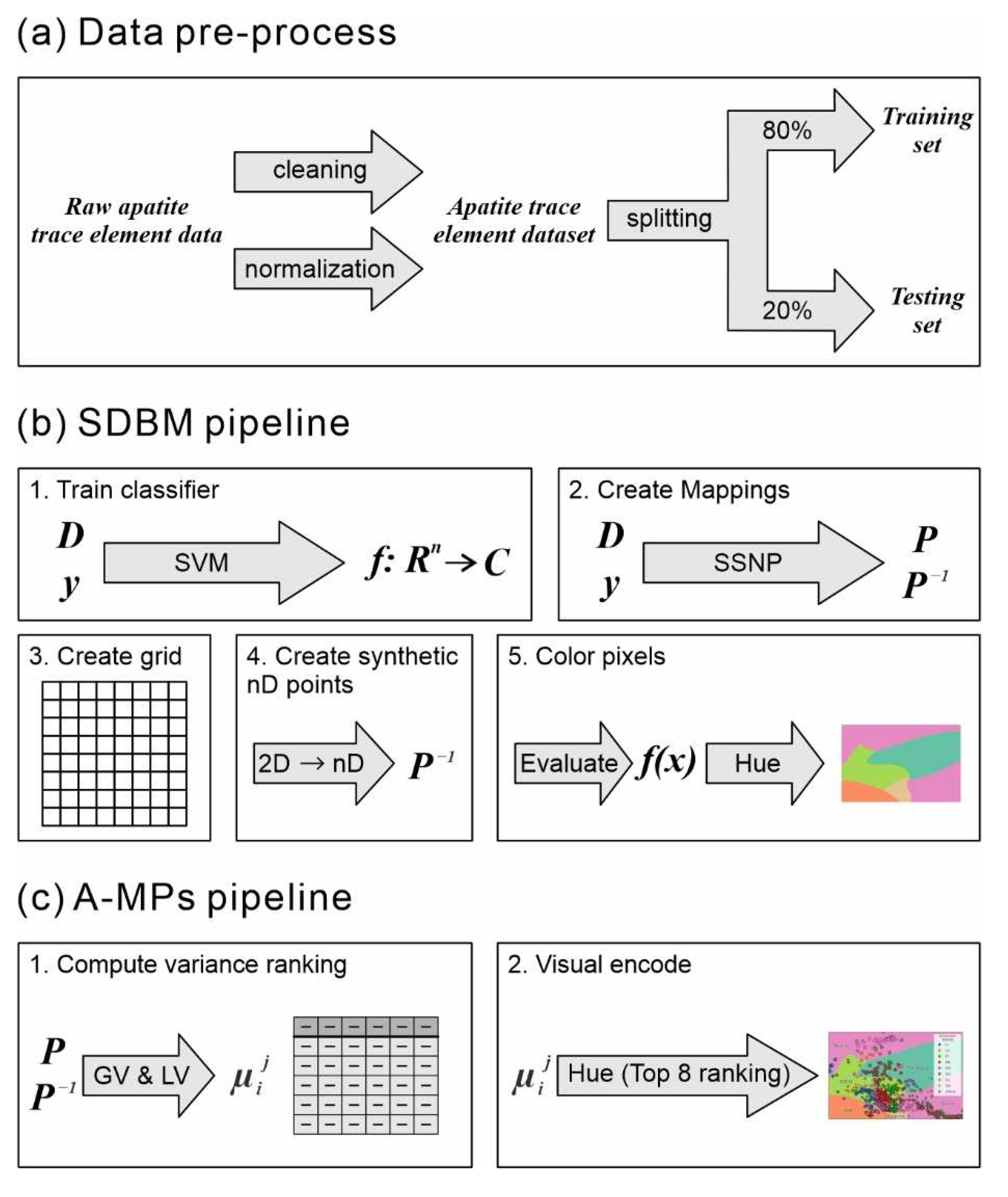
There were 534 trace element data collected from the skarn deposit, while only 78 were collected from the IOCG deposit in the apatite trace element dataset. We applied the synthetic minority oversampling technique (SMOTE) to minimize the possible effects and eliminate imbalanced data size resulting from variations in sample size in the skarn and IOCG deposit [53,54]. This did not overestimate the results, as only the training set was oversampled, using SMOTE to eliminate the effect of the imbalanced dataset. The workflow is shown in Figure 1a.
3.2. SDBM Visualization
Visualizing decision boundaries of modern machine learning classifiers can notably help in classifier design, testing, and fine-tuning [55,56]. Most visualizing methods are essentially dimensionality reduction (DR) methods: visualizing the boundaries and/or zones by projecting a high-dimensional dataset (D) to a two-dimensional scatterplot (P(D)) using projection methods (P) [12]. Based on the trained classifiers (f), similar samples (x) were grouped into the same cluster in the scatterplot. If the point P(x) is the same color, they can be considered as the same group, and vice versa. However, these 2D scatterplots have a limitation, in that it is not clear what the blank space represents.
Recently, a novel attempt called decision boundary maps (DBM) was developed to address this limitation [12,57]. The DBM method projects D to scatterplot P(D) and then inversely projects all pixels P(x) in the 2D bounding box of P(D) to create synthetic high-dimensional data points P−1(x). The points P−1(x) are classified by classifier f, and then their corresponding pixels P(x) are colored by the assigned class labels f(P−1(X)). DBM extends classical multidimensional projections by filling in the gaps between the projected points from a labeled dataset used to train a classifier [18].
More recently, a deep learning DR method called self-supervised network projection (SSNP) was proposed. SSNP is a rapid and uncomplicated method that reduces dimensions by replacing the true label with pseudo-labels assigned by some clustering algorithms [58] using the capabilities of clustering and reverse projecting. Using SSNP, DBM provides improved SDBM. Compared with DBM, SDBM produces results that are easier to interpret and use, while still having enough versatility.
As an extension of machine learning classification algorithms, SDBM provides an advanced visualization technique that depicts the high-dimensional decision space in a 2D visualized space. In this study, we used the support vector machine (SVM) [59] to train the classifier based on the apatite trace element dataset and then built SDBM to generate the decision boundary and/or zone. The workflow is shown in Figure 1b.
3.3. Attribute-Based Visual Explanation of Multidimensional Projections
We applied attribute-based visual explanation of multidimensional projections (A-MPs) to correlate the features (apatite trace elements in our study) and decision boundaries/zones [19].
There are N n-dimensional elements in the dataset D, where N is the number of the sample and n is the dimension of the dataset. The projected element is . For each 2D projected point , we first defined its 2D neighborhood as all projected points closer to than a given radius . So, an nD neighborhood of point is defined as . Then, we computed the global variance of all dimensions over all points in D (n = 14 in our study), and the local variance over for each point i. Next, for indicating the relative importance of dimensions, we computed the ratio between the local variance and global variance and normalize this ratio. Finally, we generated the rank of dimension j for point. The function is as follows:
Lower values of rank indicate a higher interpretability of dimension and homogeneity [19]. For example, if is the lowest, dimension Sr is best for explaining a local neighborhood . These points in the 2D scatterplot cluster together because the values of Sr show a high similarity in the local neighborhood .
We selected top-ranked C-dimension (C = 8 in this study) for most points and colored all the points through the classification color map. Dimensions (elements) that are top-rank for many points are mapped to distinct colors. Low number of points are not colored. These dimensions are summarized into “others”. The workflow is shown in Figure 1c.
3.4. Evaluation Metrics
Macro F1 score and accuracy are used to quantitatively evaluate the classifier and SDBM in this study. The calculation processes of the evaluation metrics are shown in Table 2 and Equations (1)–(4).
4. Results
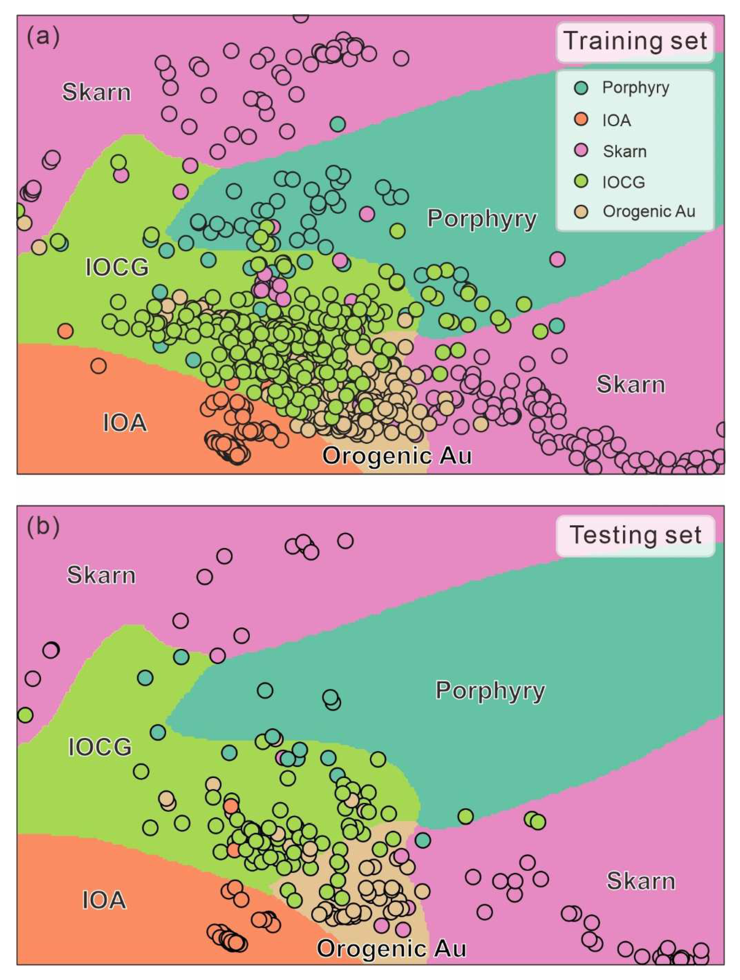
We established the optimal classifier and SDBM for the genesis classification task constructed on our dataset. The classifier could effectively distinguish the genesis of apatite with a cross-validation accuracy of 94% and test accuracy of 89% (Table 3). The IOA deposit yielded the highest F1 score and all of the analyses were predicted correctly. The accuracy of the IOCG deposit was the lowest (F1-score = 69%). SDBM was built via the SVM classifier. The overall accuracy of SDBM was ~86%, which was slightly lower than the classifier. Five genetic types of apatite were distinguished well visually and most of the analyses matched their corresponding zones. An exception was the apatite in IOCG and orogenic Au deposit, for which there was slightly overlapping (Figure 2a). A similar phenomenon was seen in the testing set (Figure 2b).
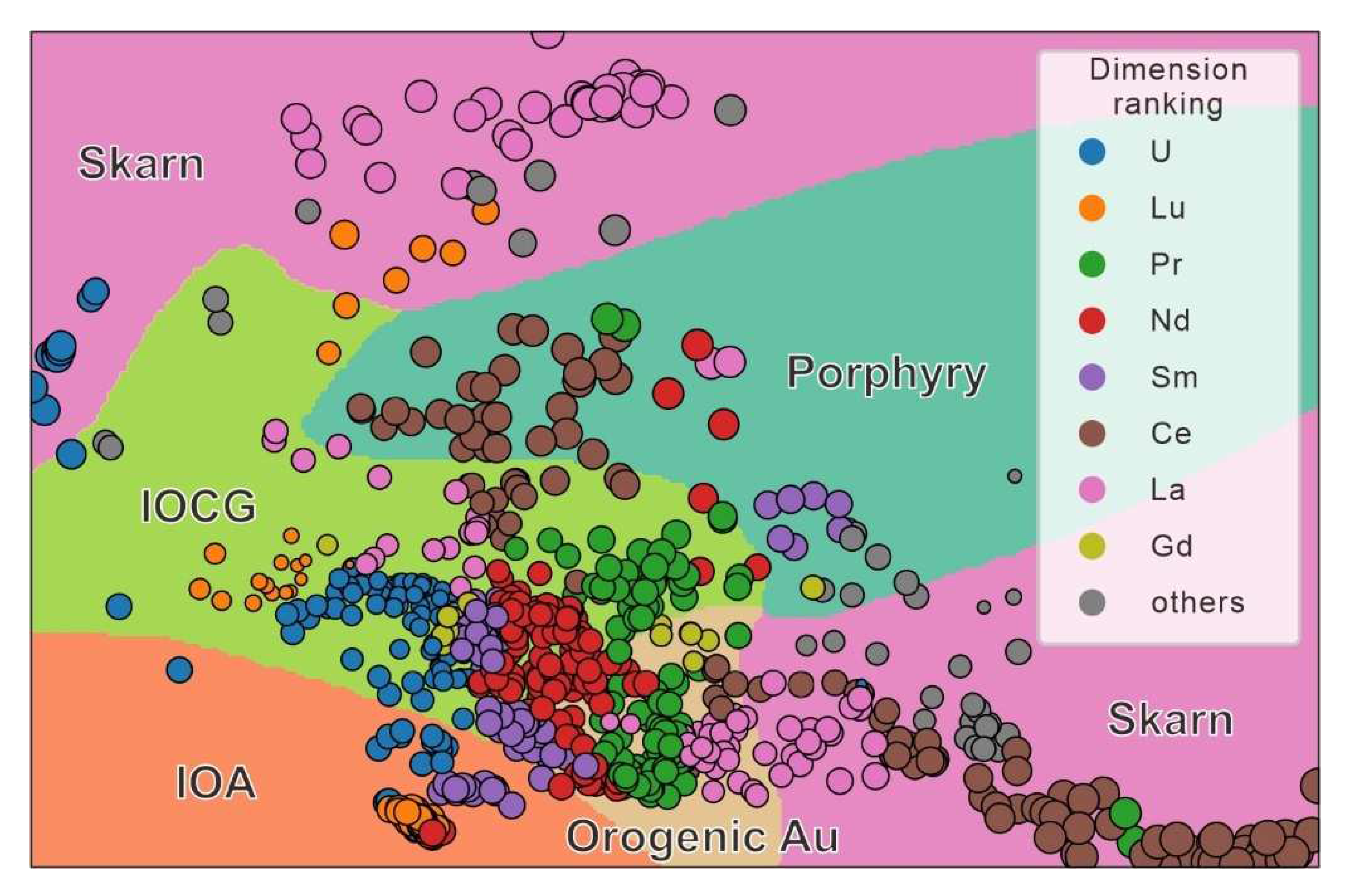
Based on the A-MPs approach, we computed the ranks of all of the dimension points and generated a visual interpretation of the SDBM diagram. All samples were colored according to the dimension (element) that contributed the most (Figure 3). The top seven dimensions that affected the clustering performance were U, Lu, Pr, Nd, Sm, Ce, and La. Most analyses clustered well on different dimensions. Eu contributed the most to the good clustering of the porphyry deposit samples after projection, and the concentration of Eu of the apatite sample in the porphyry deposit showed a high similarity. For the IOA deposit samples that performed well in the SDBM diagram, they were not controlled by one element actually, but Lu, Sm, and U simultaneously contributed the most to distinguishing IOA deposit. Samples from IOCG and orogenic Au deposit were controlled by Pr, Nd, and Sm simultaneously, which were not well distinguished.
5. Discussion
5.1. Visualization in High-Dimensional Space
Machine learning approaches are often referred to as a black box, in which the process between the input and output is invisible and unexplained [11]. SDBM offers the possibility of understanding how machine learning models work as well as an enhancement of traditional machine learning models. The shape of the decision zone and the distance of the cluster indicate the difficulty of the classification, e.g., the smooth decision boundaries represent easier classification, especially for IOA and skarn deposit [56]. Although apatite samples from skarn deposit fall into two decision zones, they have little overlap with other classes, and these two parts are clustered well separately. The performance of distinguishing apatite from the IOCG and orogenic Au deposit is relatively poor, with a large amount of apatite samples overlapping. It is the same as the result of the classifier, where the F1-score of the IOCG deposit is the lowest (Table 3).
The proximities of the samples to the closest decision boundaries represent the confidence of classification, while they are directly proportional to uncertainties. Apatite samples from the porphyry deposit are plotted near the boundary between the IOCG and porphyry deposit. Therefore, the confidence of the predicted porphyry label was relatively low, although it was well clustered (Figure 2a). Figure 2b shows that most apatite samples from the porphyry deposit in the testing set fell near the boundary. The low confidence may be mainly attributed to the complexity of porphyry mineralization processes. Because of porphyry, mineralization spanned a broad temperature range from 250 to 1000 °C; therefore, apatite crystallize in different stages of porphyry deposit may have quite different trace element signatures [60,61,62]. Apatite from the IOCG deposit is also plotted near the boundary between the IOCG and orogenic Au deposit, which also explains its low accuracy.
Despite accurate results, SDBM (DR methods) has been proven to also have some limitations. Decision zones were drawn on a specific projection plane, not on an individual dimension, and the coordinates did not represent specific features (trace elements). SDBM diagrams were not plotted in traditional two- or three-variable scatterplots. Despite this, SDBM still provided a novel way to gain insight into how machine learning works. The degree of cluster and the distance between clusters explained the predictive score of the machine learning model. Decision zones matched equally to known properties of training samples zones for the classifier [63]. A small-size “island” of one color embedded in large zones of different colors suggested misclassifications or training problems [55].
5.2. Explanation of Multidimensional Projections
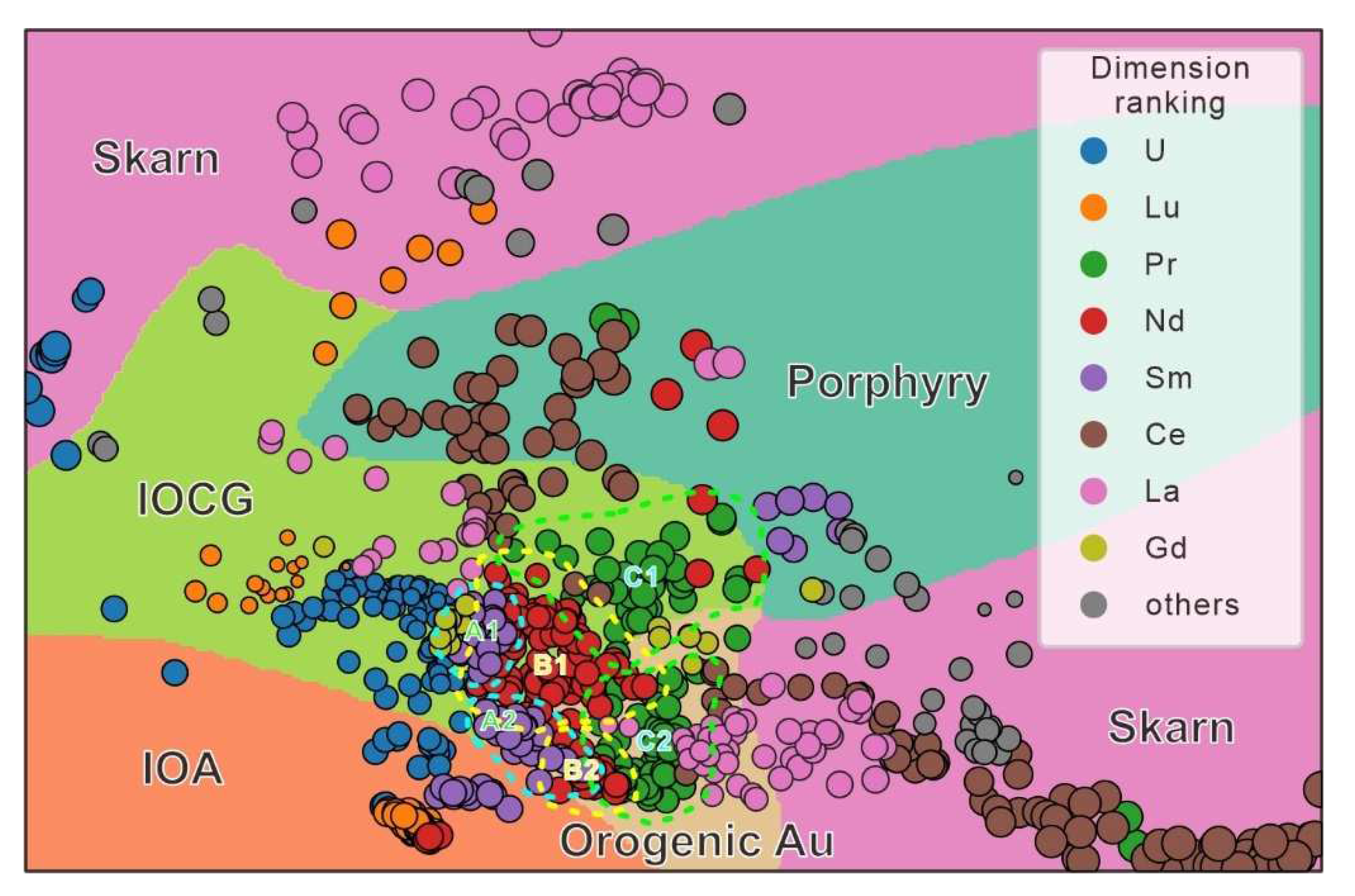
SDBM visualized the machine learning process in the high-dimensional space, and solved the “black box” problem to a certain extent. However, it still needs further studies to address the roles of the features considering the training process and the shapes of the data clusters. Based on the A-MPs approach, we described the most decisive dimensions in multidimensional projection and explained the machine learning classification [19]. SDBM showed that apatite samples in the skarn deposit fell into two decision zones (Figure 2a). Correspondingly, A-MPs also showed these two parts of the skarn deposit. Samples in the skarn deposit clustered together at the upper decision zone were mainly controlled by La, whereas samples plotted together at the lower right decision zone were mainly controlled by Ce. Furthermore, some samples from the skarn deposit were plotted at the lower right decision zone, which were controlled by La. However, these samples were located near the decision boundary and were lower than the pixel limits (Figure 4). Ce and La contributed the most to identifying the apatite from the skarn deposit.
An overlap between samples in the IOCG and orogenic Au deposit was recognized (Figure 4). The SVM classifier showed that the test score of the IOCG deposit was the lowest. The A-MPs approach showed the reason for the poor performance. The samples in the A-MPs approach were not divided into IOCG and orogenic Au clusters similar to SDBM, but the classifications of both IOCG and orogenic Au deposit were mainly controlled by Pr, Nd, and Sm. In the dimensions Pr, Nd, and Sm, samples from IOCG and orogenic Au deposit were clustered into six clusters (IOCG: A1, B1, and C1; orogenic Au: A2, B2, and C2; Figure 4). The clusters in the IOCG zone were in close proximity to clusters in orogenic Au zones, which is the reason for the overlap between the IOCG and orogenic Au deposit in the SDBM diagram. In addition, the main clusters (B1 and C1) in the IOCG zone were located near the decision boundary, while the main clusters (B2 and C2) in the orogenic Au zone were located in the middle of this decision zone. It also explains why these samples were overlapped, but the testing score of IOCG was only 69% and the testing score of orogenic Au was 89% (Table 3). Samples in the IOCG deposit were simultaneously controlled by six elements (U, Lu, Pr, Nd, Sm, and La; Figure 4), suggesting training problems. This is possible, because there may have been some issues with the apatite trace element data collected from the IOCG deposit due to the limitations of how laboratories record and publish the data.
The A-MPs approach effectively explained the role of the features (trace elements) in the machine learning process and the projection’s layout. The dimensions (elements) that were decisive for the multidimensional projections were labeled with different colors, which demonstrated the correlation between the apatite trace element data and the genetic types. Combined with the SDBM method, the A-MPs approach visualized the results of the machine learning model and solved the overlap in the IOCG and orogenic deposit.
5.3. Other Interpretation Approaches
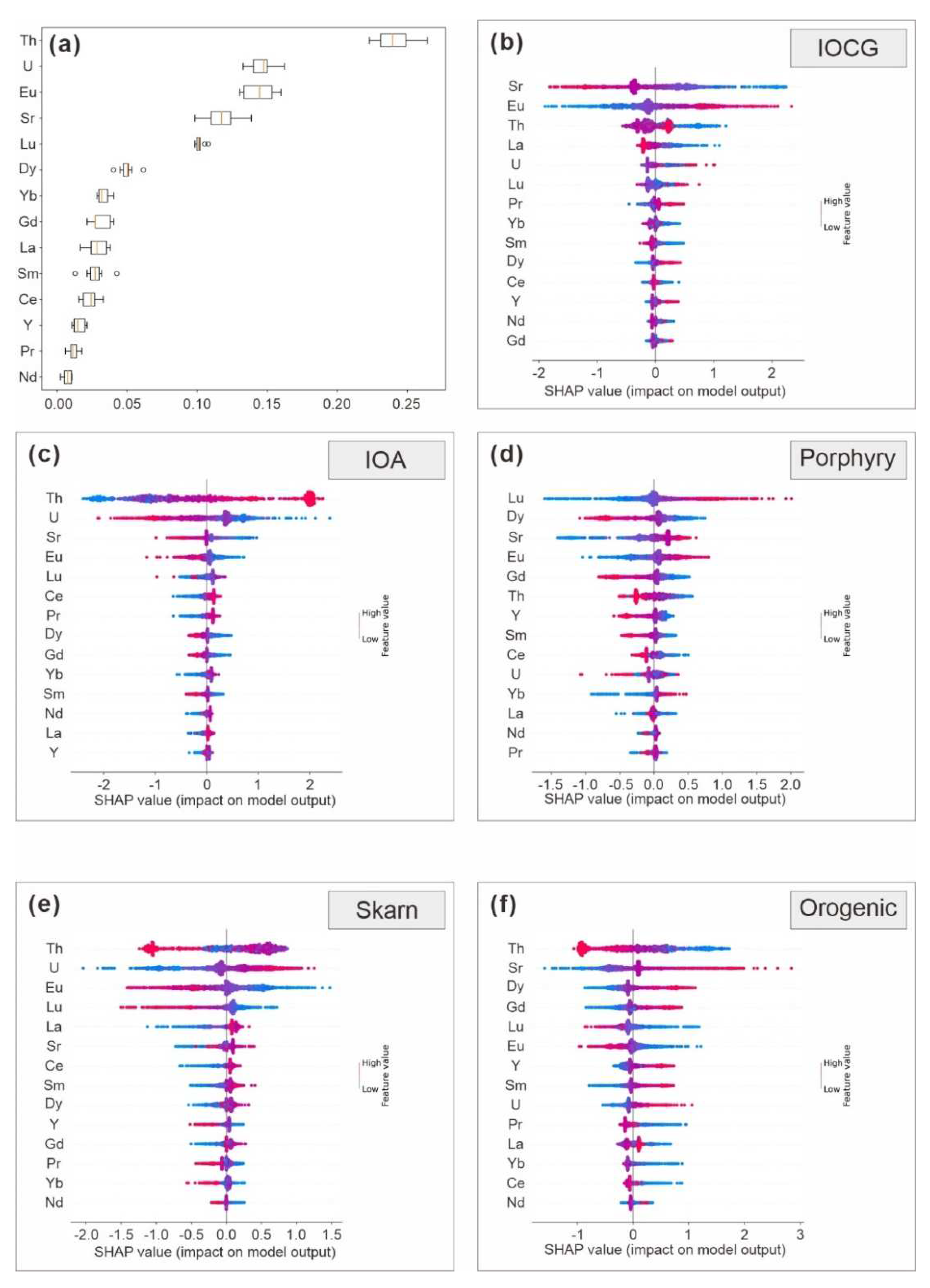
Feature importance is a model inspection technique. After a single feature in the test dataset was shuffled, the test data were reclassified. If the test score dropped, it indicated that the model depended on this feature to a great extent. Depending on how much the model performance declined, the features were listed in order from highest to lowest to find out the most effective feature for the classification [15]. Figure 5a shows that Th, U, Eu, Sr, and Lu were the most effective elements for distinguishing the ore genetic type. However, it is not clear how these five elements affected the classification and whether they had a positive or negative impact on the classification.
SHAP (SHAPley Additive exPlanations) is a game theoretic method and can explain the outputs of the machine learning models [64]. Based on the machine learning model, an interpretable model was generated. For each test sample, interpretable model generated a predicted value and assigned a numerical value (SHAP value) to each feature of the samples. Subsequently, the SHAP values were visualized and sorted in the summary plot to improve the transparency and interpretation of the machine learning models [16,65]. In different ore sources, the indicative elements were different and the concentration of elements also had an impact on the classification (Figure 5b–f). The ability to correlate element concentration with its contribution to classification was a significant advantage of SHAP [66]. Nevertheless, although SHAP displays the contribution of each sample for the classification in different classes well, it was still unclear how multiple features simultaneously controlled the classification results. For example, via Figure 5b, we found both low U and high Th were helpful to identify the IOA deposit. However, it is unknown which genetic type apatite with both low Th and U should be classified into. In addition, SDBM is an advanced multidimensional projection method, while SHAP is a game theoretic method. These two methods do not work well together.
In summary, neither feature importance nor SHAP provided a transparent working process. SDBM generated an intuitive discriminate diagram and revealed the classification process. According to the proximities of the samples to the closest decision boundaries and the shape of the decision zones, it explains why samples were distinguished to the specific class. On the basis of SDBM, A-MPs displayed control of the features over classification, including how features controlled the identification, and what roles the features played in the classification. Even in the IOCG region controlled by multiple elements, A-MPs exhibited the different characteristics played by different elements. However, SDBM also has the limitation that the correlation between the element concentration and classification interpretation could not be observed intuitively. Furthermore, the indicative features obtained by different calculation methods were not identical (A-MPs: U, Lu, and Pr; SHAP: Th, U, and Sr). The combination of SDBM with A-MPs and SHAP may have the potential to provide a more effective interpretation visualization approach.
5.4. Future Work
There were phenomena remaining in the SDBM and A-MPs diagrams. Samples from the skarn zones showed a certain trend from the lower right to upper left, and a low number of skarn samples were also located inside the IOCG field (Figure 2a). The IOA samples fell well within their assigned region (Figure 1a), while these points were divided into three clusters by U, Sm, and Lu (Figure 3). For the further research, SDBM in combination with A-MPs has the potential to explore the underlying correlation between the trace elements and the ore genetic type.
6. Conclusions
In this study, using combined SDBM and A-MPs approaches, we provide a novel machine learning visualization method with a high accuracy and strong interpretability. SDBM offers the possibility to understand how machine learning models work and intuitively and accurately distinguish apatite genetic types. A-MPs describes the dimensions that contribute the most to the post-projection clustering and demonstrates strong correlations between high-dimensional trace-element geochemical data of apatite and ore genetic types. Under the control of La and Ce, the skarn deposit is separated into two parts from the others (mainly controlled by La and mainly controlled by Ce). IOCG and orogenic Au deposit are simultaneously controlled by Pr, Nd, and Sm; thus, there are some overlap features. Our method provides a novel insight for the visualization application of geo-machine learning and is expected to be a powerful tool for high-dimensional geochemical data analysis.
Author Contributions
Conceptualization, M.-G.A.; writing, T.Z.; review and editing, M.T. and Y.-W.C.; formal analysis, F.Z., C.-L.Z. and X.-C.S. All authors have read and agreed to the published version of the manuscript.
Funding
This work was financially supported by the National Natural Science Foundation of China (42261134535 and 42072087), the Shandong Provincial Engineering Laboratory of Application and Development of Big Data for Deep Gold Exploration (SDK202211 and SDK202214), the Beijing Nova Program (Z201100006820097), and the 111 Project (BP0719021).
Data Availability Statement
Data are available upon request from the Zenodo website (https://doi.org/10.5281/zenodo.7648664).
Conflicts of Interest
The authors declare no conflict of interest.
References
- Dramsch, J.S. 70 years of machine learning in geoscience in review. Adv. Geophys. 2020, 61, 1–55. [Google Scholar]
- Bergen, K.J.; Johnson, P.A.; de Hoop, M.V.; Beroza, G.C. Machine learning for data-driven discovery in solid Earth geoscience. Science 2019, 363, eaau0323. [Google Scholar] [CrossRef]
- Kotsiantis, S.B.; Zaharakis, I.D.; Pintelas, P.E. Machine learning: A review of classification and combining techniques. Artif. Intell. Rev. 2006, 26, 159–190. [Google Scholar] [CrossRef]
- Nachtergaele, S.; De Grave, J. AI-Track-tive: Open-source software for automated recognition and counting of surface semi-tracks using computer vision (artificial intelligence). Geochronology 2021, 3, 383–394. [Google Scholar] [CrossRef]
- Wang, Y.; Qiu, K.F.; Müller, A.; Hou, Z.L.; Zhu, Z.H.; Yu, H.C. Machine learning prediction of quartz forming-environments. J. Geophys. Res. Solid Earth 2021, 126, e2021JB021925. [Google Scholar] [CrossRef]
- Chen, H.; Su, C.; Tang, Y.Q.; Li, A.Z.; Wu, S.S.; Xia, Q.K.; ZhangZhou, J. Machine learning for identification of primary water concentrations in mantle pyroxene. Geophys. Res. Lett. 2021, 48, e2021GL095191. [Google Scholar] [CrossRef]
- Gion, A.M.; Piccoli, P.M.; Candela, P.A. Characterization of biotite and amphibole compositions in granites. Contrib. Mineral. Petrol. 2022, 177, 43. [Google Scholar] [CrossRef]
- Zhong, R.; Deng, Y.; Li, W.; Danyushevsky, L.V.; Cracknell, M.J.; Belousov, I.; Chen, Y.; Li, L. Revealing the multi-stage ore-forming history of a mineral deposit using pyrite geochemistry and machine learning-based data interpretation. Ore Geol. Rev. 2021, 133, 104079. [Google Scholar] [CrossRef]
- Ziyi, Z.; Fei, Z.; Yu, W.; Tong, Z.; Zhaoliang, H.; Kunfeng, Q. Machine learning-based approach for zircon classification and genesis determination. Earth Sci. Front. 2022, 29, 464. [Google Scholar]
- Wu, Y.; Jia, M.; Xiang, C.; Fang, Y. Latent trajectories of frailty and risk prediction models among geriatric community dwellers: An interpretable machine learning perspective. BMC Geriatr. 2022, 22, 900. [Google Scholar] [CrossRef]
- Rodrigues, F.C.; Espadoto, M.; Hirata, R., Jr.; Telea, A.C. Constructing and visualizing high-quality classifier decision boundary maps. Information 2019, 10, 280. [Google Scholar] [CrossRef] [Green Version]
- Zou, C.; Zhao, L.; Xu, M.; Chen, Y.; Geng, J. Porosity prediction with uncertainty quantification from multiple seismic attributes using random forest. J. Geophys. Res. Solid Earth 2021, 126, e2021JB021826. [Google Scholar] [CrossRef]
- Roscher, R.; Bohn, B.; Duarte, M.; Garcke, J. Explain It to Me—Facing Remote Sensing Challenges in the Bio-and Geosciences With Explainable Machine Learning. ISPRS Ann. Photogramm. Remote Sens. Spat. Inf. Sci. 2020, 3, 817–824. [Google Scholar] [CrossRef]
- Nathwani, C.L.; Wilkinson, J.J.; Fry, G.; Armstrong, R.N.; Smith, D.J.; Ihlenfeld, C. Machine learning for geochemical exploration: Classifying metallogenic fertility in arc magmas and insights into porphyry copper deposit formation. Miner. Depos. 2022, 57, 1143–1166. [Google Scholar] [CrossRef]
- Al-Najjar, H.A.; Pradhan, B.; Beydoun, G.; Sarkar, R.; Park, H.-J.; Alamri, A. A novel method using explainable artificial intelligence (XAI)-based Shapley Additive Explanations for spatial landslide prediction using Time-Series SAR dataset. Gondwana Res. 2022, in press. [Google Scholar] [CrossRef]
- Chelgani, S.C. Estimation of gross calorific value based on coal analysis using an explainable artificial intelligence. Mach. Learn. Appl. 2021, 6, 100116. [Google Scholar] [CrossRef]
- Oliveira, A.A.; Espadoto, M.; Hirata, R., Jr.; Telea, A.C. SDBM: Supervised Decision Boundary Maps for Machine Learning Classifiers. In Proceedings of the VISIGRAPP (3: IVAPP), Online Streaming, 6–8 February 2022; pp. 77–87. [Google Scholar]
- Da Silva, R.R.; Rauber, P.E.; Martins, R.M.; Minghim, R.; Telea, A.C. Attribute-based Visual Explanation of Multidimensional Projections. In Proceedings of the EuroVA@ EuroVis, Sardinia, Italy, 25–26 May 2015; pp. 31–35. [Google Scholar]
- Sha, L.-K.; Chappell, B.W. Apatite chemical composition, determined by electron microprobe and laser-ablation inductively coupled plasma mass spectrometry, as a probe into granite petrogenesis. Geochim. Cosmochim. Acta 1999, 63, 3861–3881. [Google Scholar] [CrossRef]
- Zhou, T.; Qiu, K.; Wang, Y.; Yu, H.; Hou, Z. Apatite Eu/Y-Ce discrimination diagram: A big data based approach for provenance classification. Acta Petrol. Sin. 2022, 38, 291–299. [Google Scholar]
- Yu, H.-C.; Qiu, K.-F.; Hetherington, C.J.; Chew, D.; Huang, Y.-Q.; He, D.-Y.; Geng, J.-Z.; Xian, H.-Y. Apatite as an alternative petrochronometer to trace the evolution of magmatic systems containing metamict zircon. Contrib. Mineral. Petrol. 2021, 176, 68. [Google Scholar] [CrossRef]
- Qiu, K.-F.; Yu, H.-C.; Deng, J.; McIntire, D.; Gou, Z.-Y.; Geng, J.-Z.; Chang, Z.-S.; Zhu, R.; Li, K.-N.; Goldfarb, R. The giant Zaozigou Au-Sb deposit in West Qinling, China: Magmatic-or metamorphic-hydrothermal origin? Miner. Depos. 2020, 55, 345–362. [Google Scholar] [CrossRef]
- Chu, M.-F.; Wang, K.-L.; Griffin, W.L.; Chung, S.-L.; O’Reilly, S.Y.; Pearson, N.J.; Iizuka, Y. Apatite composition: Tracing petrogenetic processes in Transhimalayan granitoids. J. Petrol. 2009, 50, 1829–1855. [Google Scholar] [CrossRef]
- Yu, H.-C.; Qiu, K.-F.; Chew, D.; Yu, C.; Ding, Z.-J.; Zhou, T.; Li, S.; Sun, K.-F. Buried Triassic rocks and vertical distribution of ores in the giant Jiaodong gold province (China) revealed by apatite xenocrysts in hydrothermal quartz veins. Ore Geol. Rev. 2022, 140, 104612. [Google Scholar] [CrossRef]
- Chew, D.M.; Sylvester, P.J.; Tubrett, M.N. U–Pb and Th–Pb dating of apatite by LA-ICPMS. Chem. Geol. 2011, 280, 200–216. [Google Scholar] [CrossRef]
- Webster, J.D.; Piccoli, P.M. Magmatic apatite: A powerful, yet deceptive, mineral. Elements 2015, 11, 177–182. [Google Scholar] [CrossRef]
- Hughes, J.M.; Rakovan, J.F. Structurally robust, chemically diverse: Apatite and apatite supergroup minerals. Elements 2015, 11, 165–170. [Google Scholar] [CrossRef]
- Zhou, R.-J.; Wen, G.; Li, J.-W.; Jiang, S.-Y.; Hu, H.; Deng, X.-D.; Zhao, X.-F.; Yan, D.-R.; Wei, K.-T.; Cai, H.-A. Apatite chemistry as a petrogenetic–metallogenic indicator for skarn ore-related granitoids: An example from the Daye Fe–Cu–(Au–Mo–W) district, Eastern China. Contrib. Mineral. Petrol. 2022, 177, 23. [Google Scholar] [CrossRef]
- Mao, M.; Rukhlov, A.S.; Rowins, S.M.; Spence, J.; Coogan, L.A. Apatite trace element compositions: A robust new tool for mineral exploration. Econ. Geol. 2016, 111, 1187–1222. [Google Scholar] [CrossRef] [Green Version]
- O’Sullivan, G.; Chew, D.; Kenny, G.; Henrichs, I.; Mulligan, D. The trace element composition of apatite and its application to detrital provenance studies. Earth Sci. Rev. 2020, 201, 103044. [Google Scholar] [CrossRef]
- Belousova, E.; Griffin, W.; O’Reilly, S.Y.; Fisher, N. Apatite as an indicator mineral for mineral exploration: Trace-element compositions and their relationship to host rock type. J. Geochem. Explor. 2002, 76, 45–69. [Google Scholar] [CrossRef]
- Deng, J.; Yang, L.-Q.; Groves, D.I.; Zhang, L.; Qiu, K.-F.; Wang, Q.-F. An integrated mineral system model for the gold deposits of the giant Jiaodong province, eastern China. Earth Sci. Rev. 2020, 208, 103274. [Google Scholar] [CrossRef]
- Qiu, K.-F.; Yu, H.-C.; Hetherington, C.; Huang, Y.-Q.; Yang, T.; Deng, J. Tourmaline composition and boron isotope signature as a tracer of magmatic-hydrothermal processes. Am. Mineral. J. Earth Planet. Mater. 2021, 106, 1033–1044. [Google Scholar] [CrossRef]
- Wu, M.; Samson, I.; Qiu, K.; Zhang, D. Concentration mechanisms of REE-Nb-Zr-Be mineralization in the Baerzhe deposit, NE China: Insights from textural and chemical features of amphibole and rare-metal minerals. Econ. Geol. 2021, 116, 651–679. [Google Scholar] [CrossRef]
- Li, C.; Arndt, N.T.; Tang, Q.; Ripley, E.M. Trace element indiscrimination diagrams. Lithos 2015, 232, 76–83. [Google Scholar] [CrossRef]
- Pearce, J.A. A user’s guide to basalt discrimination diagrams. In Trace Element Geochemistry of Volcanic Rocks: Applications for Massive Sulphide Exploration. Geological Association of Canada, Short Course Notes; Geological Association of Canada: St. John’s, NL, Canada, 1996; Volume 12, p. 113. [Google Scholar]
- Snow, C.A. A reevaluation of tectonic discrimination diagrams and a new probabilistic approach using large geochemical databases: Moving beyond binary and ternary plots. J. Geophys. Res. Solid Earth 2006, 111. [Google Scholar] [CrossRef] [Green Version]
- Andersson, S.S.; Wagner, T.; Jonsson, E.; Fusswinkel, T.; Whitehouse, M.J. Apatite as a tracer of the source, chemistry and evolution of ore-forming fluids: The case of the Olserum-Djupedal REE-phosphate mineralisation, SE Sweden. Geochim. Cosmochim. Acta 2019, 255, 163–187. [Google Scholar] [CrossRef]
- Li, R.; Xu, Z.; Su, C.; Yang, R. Automatic identification of semi-tracks on apatite and mica using a deep learning method. Comput. Geosci. 2022, 162, 105081. [Google Scholar] [CrossRef]
- Cao, M.; Li, G.; Qin, K.; Seitmuratova, E.Y.; Liu, Y. Major and trace element characteristics of apatites in granitoids from Central Kazakhstan: Implications for petrogenesis and mineralization. Resour. Geol. 2012, 62, 63–83. [Google Scholar] [CrossRef]
- Pan, L.-C.; Hu, R.-Z.; Wang, X.-S.; Bi, X.-W.; Zhu, J.-J.; Li, C. Apatite trace element and halogen compositions as petrogenetic-metallogenic indicators: Examples from four granite plutons in the Sanjiang region, SW China. Lithos 2016, 254, 118–130. [Google Scholar] [CrossRef]
- Xing, K.; Shu, Q.; Lentz, D.R. Constraints on the formation of the giant Daheishan porphyry Mo deposit (NE China) from whole-rock and accessory mineral geochemistry. J. Petrol. 2021, 62, egab018. [Google Scholar] [CrossRef]
- Adlakha, E.; Hanley, J.; Falck, H.; Boucher, B. The origin of mineralizing hydrothermal fluids recorded in apatite chemistry at the Cantung W–Cu skarn deposit, NWT, Canada. Eur. J. Mineral. 2018, 30, 1095–1113. [Google Scholar] [CrossRef]
- Yang, J.-H.; Kang, L.-F.; Peng, J.-T.; Zhong, H.; Gao, J.-F.; Liu, L. In-situ elemental and isotopic compositions of apatite and zircon from the Shuikoushan and Xihuashan granitic plutons: Implication for Jurassic granitoid-related Cu-Pb-Zn and W mineralization in the Nanling Range, South China. Ore Geol. Rev. 2018, 93, 382–403. [Google Scholar] [CrossRef]
- Jia, F.; Zhang, C.; Liu, H.; Meng, X.; Kong, Z. In situ major and trace element compositions of apatite from the Yangla skarn Cu deposit, southwest China: Implications for petrogenesis and mineralization. Ore Geol. Rev. 2020, 127, 103360. [Google Scholar] [CrossRef]
- Zhang, F.; Li, W.; White, N.C.; Zhang, L.; Qiao, X.; Yao, Z. Geochemical and isotopic study of metasomatic apatite: Implications for gold mineralization in Xindigou, northern China. Ore Geol. Rev. 2020, 127, 103853. [Google Scholar] [CrossRef]
- Hazarika, P.; Mishra, B.; Pruseth, K.L. Scheelite, apatite, calcite and tourmaline compositions from the late Archean Hutti orogenic gold deposit: Implications for analogous two stage ore fluids. Ore Geol. Rev. 2016, 72, 989–1003. [Google Scholar] [CrossRef]
- Krneta, S.; Cook, N.J.; Ciobanu, C.L.; Ehrig, K.; Kontonikas-Charos, A. The Wirrda Well and Acropolis prospects, Gawler Craton, South Australia: Insights into evolving fluid conditions through apatite chemistry. J. Geochem. Explor. 2017, 181, 276–291. [Google Scholar] [CrossRef]
- Mukherjee, R.; Venkatesh, A. Chemistry of magnetite-apatite from albitite and carbonate-hosted Bhukia Gold Deposit, Rajasthan, western India—An IOCG-IOA analogue from Paleoproterozoic Aravalli Supergroup: Evidence from petrographic, LA-ICP-MS and EPMA studies. Ore Geol. Rev. 2017, 91, 509–529. [Google Scholar] [CrossRef]
- Rebala, G.; Ravi, A.; Churiwala, S. Machine learning definition and basics. In Introduction to Machine Learning; Springer: Cham, Switzerland, 2019; pp. 1–17. [Google Scholar]
- Parsons, V.L. Stratified sampling. In Wiley StatsRef: Statistics Reference Online; Wiley: Hoboken, NJ, USA, 2014; pp. 1–11. [Google Scholar]
- Chawla, N.V.; Bowyer, K.W.; Hall, L.O.; Kegelmeyer, W.P. SMOTE: Synthetic minority over-sampling technique. J. Artif. Intell. Res. 2002, 16, 321–357. [Google Scholar] [CrossRef]
- He, H.; Garcia, E.A. Learning from imbalanced data. IEEE Trans. Knowl. Data Eng. 2009, 21, 1263–1284. [Google Scholar]
- Espadoto, M.; Rodrigues, F.C.M.; Telea, A.C. Visual Analytics of Multidimensional Projections for Constructing Classifier Decision Boundary Maps. In Proceedings of the VISIGRAPP (3: IVAPP), Prague, Czech Republic, 25–27 February 2019; pp. 28–38. [Google Scholar]
- Rodrigues, F.C. Visual Analytics for Machine Learning. Ph.D. Thesis, University of Groningen, Groningen, The Netherlands, 2020. [Google Scholar]
- Rodrigues, F.C.M.; Hirata, R.; Telea, A.C. Image-based visualization of classifier decision boundaries. In Proceedings of the 2018 31st SIBGRAPI Conference on Graphics, Patterns and Images (SIBGRAPI), Paraná, Brazil, 29 October–1 November 2018; pp. 353–360. [Google Scholar]
- Espadoto, M.; Hirata, N.S.T.; Telea, A.C. Self-Supervised Dimensionality Reduction with Neural Networks and Pseudo-Labeling. In IVAPP; Hurter, C., Purchase, H., Braz, J., Bouatouch, K., Eds.; SciTePress: Setúbal, Portugal, 2021; pp. 27–37. [Google Scholar]
- Cortes, C.; Vapnik, V. Support-vector networks. Mach. Learn. 1995, 20, 273–297. [Google Scholar] [CrossRef]
- Bouzari, F.; Hart, C.; Barker, S.; Bissig, T. Exploration for concealed deposits using porphyry indicator minerals (PIMs): Application of apatite texture and chemistry [abs.]. 25th Int. Appl. Geochem. Sympos. 2011, 92, 89–90. [Google Scholar]
- Sillitoe, R.H. Porphyry copper systems. Econ. Geol. 2010, 105, 3–41. [Google Scholar] [CrossRef] [Green Version]
- Qiu, K.-F.; Taylor, R.D.; Song, Y.-H.; Yu, H.-C.; Song, K.-R.; Li, N. Geologic and geochemical insights into the formation of the Taiyangshan porphyry copper–molybdenum deposit, Western Qinling Orogenic Belt, China. Gondwana Res. 2016, 35, 40–58. [Google Scholar] [CrossRef]
- Espadoto, M.; Rodrigues, F.; Hirata, N.S.T.; Telea, A.C. Deep learning inverse multidimensional projections. In Proceedings of the 10th International EuroVis Workshop on Visual Analytics, Porto, Portugal, 3 June 2019. [Google Scholar] [CrossRef]
- Lundberg, S.M.; Lee, S.-I. A unified approach to interpreting model predictions. Adv. Neural Inf. Process. Syst. 2017, 30, 4768–4777. [Google Scholar]
- Zhou, T.; Qiu, K.-F.; Wang, Y. From Trace Elements to Petrogenesis: A Machine Learning Approach to Determine Ore Deposit Type from Trace Elements Analysis of Apatite. In Proceedings of the Copernicus Meetings, Vienna, Austria, 23–28 April 2023. [Google Scholar]
- Qiu, K.-F.; Zhou, T.; Chew, D.; Hou, Z.L.; Müller, A.; Yu, H.-C.; Lee, R.G.; Chen, H.; Deng, J. Apatite trace element composition as an indicator of ore deposit types: A machine learning approach. Am. Mineral. 2023. accepted. [Google Scholar]
- Parsa, A.B.; Movahedi, A.; Taghipour, H.; Derrible, S.; Mohammadian, A.K. Toward safer highways, application of XGBoost and SHAP for real-time accident detection and feature analysis. Accid. Anal. Prev. 2020, 136, 105405. [Google Scholar] [CrossRef]
Figure 1.
Data process workflow. (a) Data pre-process. (b) SDBM pipeline (after [18]). y is labels of the dataset as the genetic types of apatite. f(x) is evaluation metrics of accuracy and f1 score. The generated colored diagram is SDBM (The clear SDBM is shown in Figure 2. The remaining parameters are described in the text. (c) A-MPs pipeline. The generated colored diagram is visual encoding of A-MPs (The clear plot is shown in Figure 3).

Figure 2.
Supervised decision boundary map generated by the training set and the trained SVM. (a) SDBM with training set. (b) SDBM with testing set. IOCG—iron oxide copper gold deposit; IOA—iron oxide apatite deposit.
Figure 2.
Supervised decision boundary map generated by the training set and the trained SVM. (a) SDBM with training set. (b) SDBM with testing set. IOCG—iron oxide copper gold deposit; IOA—iron oxide apatite deposit.

Figure 3.
Attribute-based visual explanation of multidimensional projections. Elements that are top-rank for numerous points are mapped to distinct colors. Other—Eu, Dy, Yb, Sr, Y, and Th.
Figure 3.
Attribute-based visual explanation of multidimensional projections. Elements that are top-rank for numerous points are mapped to distinct colors. Other—Eu, Dy, Yb, Sr, Y, and Th.

Figure 4.
A-MPs diagram. A1, B1, and C1 are clusters of apatite samples in the IOCG deposit, and A2, B2, and C2 were clusters of apatite samples in the orogenic Au deposit.
Figure 4.
A-MPs diagram. A1, B1, and C1 are clusters of apatite samples in the IOCG deposit, and A2, B2, and C2 were clusters of apatite samples in the orogenic Au deposit.

Figure 5.
Feature importance scores and SHAP values generated by SVM. (a) Feature importance scores. (b–f) SHAP summary plots of apatite from various ore sources. A small circle (dot) represents an individual analysis and the color represents the concentration of the respective element (red = high, blue = low).


Table 1.
Apatite trace element dataset used in this study.
| Deposit Type | Number of Apatite Samples | Source Deposit | Reference |
|---|---|---|---|
| Porphyry | 422 | Boss Mountain, Brenda, Cassiar Moly, Daheishan, Dobbin, Endako, Gibraltar, Highland Valley, Highmont, Kemess South, Lornex, Mount Polley, Shiko, and Willa | [30,41,42,43] |
| Skarn | 534 | Cantung, Gold Canyon, Little Billie, Minyari, Molly, O’Callagham’s, Racine, Shuikoushan, and Yangla | [30,41,44,45,46] |
| Orogenic Au | 250 | Congress (Lou), Dentonia, Hutti, Kirkland Lake, Laodou, Seabee, and Xindigou | [30,47,48] |
| IOCG | 78 | Acropolis prospect, Bhukia, Wernecke, ad Wirrda Well prospect | [30,49,50] |
| IOA | 267 | Aoshan, Durango, and Great Bear | [30] |
Table 2.
Model prediction.
| Predicted Label | Positive | Negative | |
|---|---|---|---|
| True Label | |||
| Positive | True Positive (TP) | False Negative (FN) | |
| Negative | False Positive (FP) | True Negative (TN) | |
Table 3.
Classification results.
| Precision | Recall | F1-Score | Support | |
|---|---|---|---|---|
| IOCG | 0.67 | 0.71 | 0.69 | 14 |
| IOA | 1.00 | 1,00 | 1.00 | 40 |
| Orogenic | 0.89 | 0.89 | 0.89 | 44 |
| Porphyry | 0.91 | 0.89 | 0.90 | 70 |
| Skarn | 0.82 | 0.84 | 0.83 | 44 |
| Accuracy | 0.89 | 212 | ||
| Macro avg | 0.86 | 0.87 | 0.86 | 212 |
| Weighted avg | 0.89 | 0.89 | 0.89 | 212 |
Disclaimer/Publisher’s Note: The statements, opinions and data contained in all publications are solely those of the individual author(s) and contributor(s) and not of MDPI and/or the editor(s). MDPI and/or the editor(s) disclaim responsibility for any injury to people or property resulting from any ideas, methods, instructions or products referred to in the content. |
© 2023 by the authors. Licensee MDPI, Basel, Switzerland. This article is an open access article distributed under the terms and conditions of the Creative Commons Attribution (CC BY) license (https://creativecommons.org/licenses/by/4.0/).
Share and Cite
MDPI and ACS Style
Zhou, T.; Cai, Y.-W.; An, M.-G.; Zhou, F.; Zhi, C.-L.; Sun, X.-C.; Tamer, M. Visual Interpretation of Machine Learning: Genetical Classification of Apatite from Various Ore Sources. Minerals 2023, 13, 491. https://doi.org/10.3390/min13040491
AMA Style
Zhou T, Cai Y-W, An M-G, Zhou F, Zhi C-L, Sun X-C, Tamer M. Visual Interpretation of Machine Learning: Genetical Classification of Apatite from Various Ore Sources. Minerals. 2023; 13(4):491. https://doi.org/10.3390/min13040491
Chicago/Turabian StyleZhou, Tong, Yi-Wei Cai, Mao-Guo An, Fei Zhou, Cheng-Long Zhi, Xin-Chun Sun, and Murat Tamer. 2023. "Visual Interpretation of Machine Learning: Genetical Classification of Apatite from Various Ore Sources" Minerals 13, no. 4: 491. https://doi.org/10.3390/min13040491
Note that from the first issue of 2016, this journal uses article numbers instead of page numbers. See further details here.