Application of Non-Destructive Test Results to Estimate Rock Mechanical Characteristics—A Case Study

Abstract

Accurately determining rock elastic modulus (EM) and uniaxial compressive strength (UCS) using laboratory methods requires considerable time and cost. Hence, the development of models for estimating the mechanical properties of rock is a very attractive alternative. The current research was conducted to predict the UCS and EM of sandstone rocks using quartz%, feldspar%, fragments%, compressional wave velocity (PW), the Schmidt hardness number (SN), porosity, density, and water absorption via simple regression, multivariate regression (MVR), K-nearest neighbor (KNN), support vector regression (SVR) with a radial basis function, the adaptive neuro-fuzzy inference system (ANFIS) using the Gaussian membership (GM) function, and the back-propagation neural network (BPNN) based on various training algorithms. The samples were categorized as litharenite and feldspathic litharenite. By increasing the feldspar% and quartz% and decreasing the fragments%, the static properties increased. The results of the statistical analysis showed that the SN and porosity have the greatest effect on the UCS and EM, respectively. Among the Levenberg–Marquardt (LM), Bayesian regularization, and Scaled Conjugate Gradient training algorithms using the BPNN method, the LM achieved the best results in forecasting the UCS and EM. The ideal obtained BPNN, using a trial-and-error process, contains four neurons in a hidden layer with eight inputs. All five models attained acceptable accuracy (correlation coefficient greater than 70%) for estimating the static properties. By comparing the methods, the ANFIS showed higher precision than the other methods. The UCS and EM of the samples can be determined with very high accuracy (R² > 99%).

1. Introduction

The elastic modulus (EM) is a measure of a material’s stiffness, indicating how much a material will deform under stress. This property is critical for understanding how materials will behave under loads and for designing structures that can withstand stress without breaking. Uniaxial compressive strength (UCS) is a measure of a material’s ability to withstand compressive forces along a single axis. This property is essential for designing structures that can support weight or resist compression forces, such as foundations, columns, and walls. Uniaxial compressive strength is also used to evaluate rock formations for mining, drilling, and excavation operations. The UCS and EM of rocks have widespread applications in rock mass classifications, numerical modeling, and slope stability analysis. Due to problems such as obtaining appropriate samples without joints and cracks and the expensive and time-consuming UCS test, researchers tried to estimate these properties using experimental relationships and models [1,2,3].

Several relationships were suggested for estimating the UCS and EM using compressional wave velocity (PW), porosity, density, water absorption, and moisture of the sedimentary rocks [1,4,5]. Some of the experimental relationships for sedimentary rocks, particularly sandstones, are presented in

Table 1. Suggested equations for forecasting UCS and EM of sedimentary rocks.

Equation	References	Lithology	Equation No.
UCS = 0.00021 × SN33.55	Yilmaz and Goktan [28]	Different rocks	(1)
UCS = 0.00004 SN4.164	Daoud et al. [29]	Limestone and sandstone	(2)
UCS = 287.7$\rho$ − 615.90	Mishra and Basu [30]	Sandstone rocks	(3)
UCS = 0.05 PW − 126.40	Mishra and Basu [30]	Sandstone rocks	(4)
$\mathrm{U}\mathrm{C}\mathrm{S}=12.59\mathrm{I}{\mathrm{s}}_{\left(50\right)}-5.19$	Mishra and Basu [30]	Sandstone rocks	(5)
UCS = 22.18 PW − 30.32	Selçuk and Yabalak [31]	Various rocks, including sandstones	(6)
UCS = 17.783 PW1.099 (MPa)	Armaghani et al. [32]	Sandstone rocks	(7)
UCS = 0.041 PW − 15.40	Abdi and Khanlari [33]	Sandstone rocks	(8)
EM = 0.005 PW + 0.621	Abdi and Khanlari [33]	Sandstone rocks	(9)
UCS = 1.41 + 17.98exp(−19.01n)	Eremin [34]	Sandstone rocks	(10)
EM = 11.237 PW − 6.894	Bejarbaneh et al. [35]	Sandstone rocks	(11)
EM = 2.06 PW2.78	Moradian and Behnia [36]	Various rocks, including sandstone	(12)
UCS = 2.304 PW2.43	Kılıç and Teyman [37]	Various rocks, including sandstone	(13)
UCS = 56.71 PW − 192.93	Cobanoglu and Celik [38]	Sandstone and limestone	(14)
UCS = 2.56EXP(0.063SN)	Hebib et al. [39]	Sedimentary rocks	(15)
UCS = 0.007 × SN3.443	Bolla and Paronuzzi [40]	Sedimentary rocks	(16)

(Equations (1)–(16)). Due to the diversity in lithological composition, sandstones show different behaviors [5,6]. Lawal et al. [7] predicted the static properties of sedimentary rocks using intelligent methods. Armaghani et al. [8] used some index tests to predict rock mechanical properties via a BPNN. Various scholars have indicated that the SVR and BPNN perform highly in modeling rock characteristics [8,9,10,11]. Siddig et al. [12] forecasted sedimentary rock properties via the ANN and SVR methods. Zoveidavianpoor et al. [13] used the ANFIS and multilayer perceptron (MLP) methods for forecasting the PW of rocks. Mahmoodzadeh et al. [11] used KNN, SVR, and other intelligent methods to estimate the UCS of the different rocks. Chang et al. [14] reviewed the research of other researchers and presented eleven experimental relationships between the UCS of the sandstones and their physical properties. Heidari et al. [15] investigated the correlation of petrography with the UCS and EM of Jurassic sandstone rocks and presented some relationships. Wang et al. [16] applied various nonlinear models, including the SVR, BPNN, and random forest, to predict the UCS of weakly cemented Jurassic rocks. They found that the SVR had the best performance in predicting UCS values. Shahani et al. [17] used soft computing methods, including the ANFIS and genetic programming, to estimate the UCS and elastic modulus of soft sedimentary rocks. They found that the ANFIS produced more accurate results than genetic programming. Cemiloglu et al. [18] employed the SVR to predict the UCS of Maragheh limestone. They found that the SVR model had higher accuracy when compared to the multiple linear regression model. Abdelhedi et al. [19] used machine learning techniques, including the BPNN and decision trees, to predict the UCS of carbonate rocks. They found that the artificial neural network model had the best performance in predicting UCS values. Asare et al. [20] developed a hybrid intelligent prediction model, which combined an autoencoder neural network and a multivariate adaptive regression spline to predict the UCS of rocks. They reported that the proposed model outperformed other traditional models, such as the SVM and BPNN models. Wang et al. [21] developed two hybrid algorithms, which combined the BPNN with the SVR and the decision tree to predict the elastic modulus of intact rocks. They found that the proposed models were more accurate than the individual models. Zhao et al. [22] utilized deep learning techniques to predict the strength of rock by adopting measurements while drilling data. They reported that the deep learning model produced accurate and reliable predictions of rock strength. Rahman and Sarkar [23] developed empirical correlations between the UCS and the density of rocks based on lithology. They applied statistical and machine learning techniques to evaluate the performance of the developed correlations. They found that the developed empirical correlations accurately predicted the UCS of rocks. Weng and Li [24] investigated the relationships between the mechanical properties and porosity of sandstone. The results of the research by Naresh et al. [25] on Himalaya sandstones in the Nepal area showed that the percentage of porosity and petrographic properties have a high impact on the mechanical properties. Ghobadi et al. [26] studied the sandstone characteristics of the Aghajari formation and presented high-precision relationships to estimate the EM and UCS. Qi et al. [27] studied the geotechnical properties of the sandstones in the Ordos region in China.

The current research aimed to estimate the UCS and EM of sandstones based on quartz%, feldspar%, fragments%, PW, water absorption%, SN, porosity, and density using statistical analysis, MVR, SVR, and the BPNN, KNN, and ANFIS methods. Hence, microscopic studies and ultrasonic, UCS, and physical tests were conducted on specimens.

2. Materials and Methods

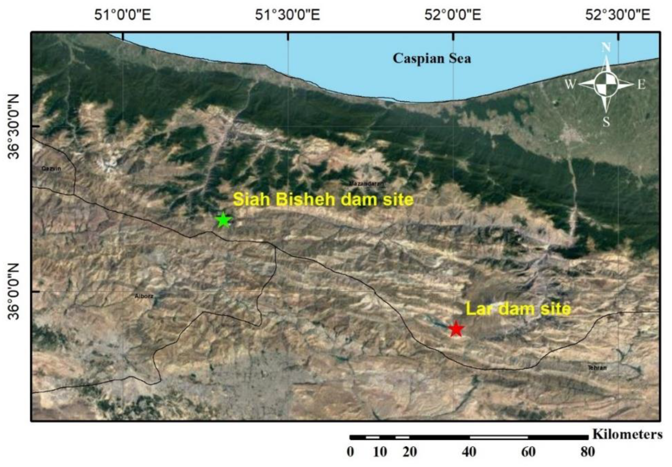
2.1. Case Study

Samples were taken from the Lar and Siah Bisheh dam sites. Lar dam is situated 75 km northeast of Tehran. The Siah Bisheh dam site is a hydroelectric power plant on the Alborz mountain range, located 125 km north of Tehran (Figure 1). The studied sandstones form the foundation of large projects in the west of Plour and Tiz Kooh, the Kandovan tunnel, and many projects in the north of Tehran.

2.2. Materials

Samples were transferred to the Environmental Data-Processors Laboratory, Tehran, Iran, for conducting experiments. Healthy cores were chosen to avoid the effect of discontinuities on the test results. Based on the ISRM standard, the diameter of the specimens is the NX size (54 mm) [41]. Additionally, the height-to-diameter ratio of the specimens is near 2.5 [41].

2.3. Methods

In this research, the Schmidt hardness number (SN), UCS, ultrasonic density, porosity, water absorption, and also thin-section tests were performed on 64 samples. According to the presented peaks in the X-ray diffraction (XRD) diagram, the types and amounts of the mineral were determined. The ultrasonic experiment was performed to measure the velocity of the compressional wave [42]. Wave velocity was measured using the wavelength of the wave and the distance between the wave receiver and transmitter. The frequency used in these tests is 0.5 MHz. The wave speed of the intact rock depends on the grain size, density, porosity, degree of saturation, type and orientation of minerals, and temperature [43,44].

An N-type hammer (Tiss Company, Tehran, Iran) was used to perform the Schmidt hammer test. In this test, the mode of operation is such that by a spring under tension, a certain force is applied to the part of the hammer that is placed in the vicinity of the sample. The amount of reflected energy from the joint between the rock and the hammer is measured by the return value of the hammer. This test is used to determine the hardness of the rocks in the field or laboratory. Using the Schmidt hardness number, the compressive strength of the rock can be estimated [31]. This test was performed in the laboratory on 64 cores. Finally, the average of 10 numbers in a range was determined for each sample. The Schmidt hammer is vertically used in all the studied samples in this research.

The density, porosity (%), and water absorption by weight (%) of the specimens were measured [41]. In order to determine the porosity of the studied specimens, the saturation-buoyancy method was used. The UCS test was performed according to the ASTM standard [45] and with a 0.80 MPa/S loading rate on the specimens. The amount of deformation was recorded using the relevant gauges in the UCS test. The curves of stress and strain were then drawn to determine the UCS and EM. The EM was determined based on the conception of the secant modulus.

2.4. Data Normalization

Before modeling by using intelligent methods, all data were normalized between −1 and 1 using Equation (17) to prevent data size effects on the trained BPNN.

$${\mathrm{X}}_{\mathrm{i}}=2\left(\frac{{\mathrm{X}-\mathrm{X}}_{\min }}{{\mathrm{X}}_{\max }{-\mathrm{X}}_{\min }}\right)-1$$

(17)

where X, X_min, and X_max are measured values, minimum data, and maximum data, respectively. The estimated UCS and EM precision were appraised using R² and RMSE.

2.5. The SVR Approach

The SVR approach matched a curve with epsilon ($\epsilon$) width on the model to obtain the lowest error [46]. Functions, including f(x) = W.x + B, were used for predicting in this method, where x and B are the bias values, and W is the weight vector. The appropriate error function was used by SVR to eliminate errors within a certain range of the real values. As a result, by minimizing the weight vector, the model test error is minimized. Hence, deviation from epsilon, which is determined by Equation (18), must be overlooked. By including Equation (18) in Equation (19), the ${\xi }_i^{+}$ and ${\xi }_i^{-}$ deficiency parameters are considered. According to the principle of structural error minimization, the error values are finally optimized via Equation (19) [11,47].

$${\left|\xi \right|}_{\epsilon }=\left[\begin{array}{l}0\hspace{1em}\hspace{1em}\hspace{1em}\hspace{1em}\hspace{1em}\hspace{1em}\hspace{1em}\hspace{1em}if\left|\xi \right|\le \epsilon \\ \left|\xi \right|-\epsilon \hspace{1em}\hspace{1em}otherwise\end{array}\right]$$

(18)

$$\begin{gathered} \mathrm{Minimize}: \frac{1}{2}{\Vert W\Vert }^2+\mathrm{C}{\displaystyle {\sum }_{i=1}^N({\xi }_i^{+}}+{\xi }_i^{-}) \\ {\epsilon }_{\mathrm{Constrains}}: \left[\begin{array}{l}\mathrm{W}.{\mathrm{x}}_{\mathrm{i}}+\mathrm{B}-{\mathrm{y}}_{\mathrm{i}}\le \mathsf{\epsilon }+{\mathsf{\xi }}_{\mathrm{i}}^{+}\hspace{1em}\hspace{1em}\hspace{1em}\hspace{1em}\mathrm{i}=1,2,\dots ,\mathrm{N}\\ {\mathrm{y}}_{\mathrm{i}}-(\mathrm{W}.{\mathrm{x}}_{\mathrm{i}}+\mathrm{B})\le \mathsf{\epsilon }+{\mathsf{\xi }}_{\mathrm{i}}^{-}\hspace{1em}\hspace{1em}\hspace{1em}\mathrm{i}=1,2,\dots ,\mathrm{N}\\ {\mathsf{\xi }}_{\mathrm{i}}^{+}\ge 0,{\mathsf{\xi }}_{\mathrm{i}}^{-}\ge 0\hspace{1em}\hspace{1em}\hspace{1em}\hspace{1em}\hspace{1em}\hspace{1em}\mathrm{i}=1,2,\dots ,\mathrm{N}\end{array}\right] \end{gathered}$$

(19)

where $\frac{1}{2} {\Vert W\Vert }^2$ is the regulatory equation section, N is the sample number, C is the complexity balance coefficient, and ε is the acceptable error. Among the polynomial, linear, quadratic, and radial kernel functions used in the SVR method, the radial has shown the best efficiency for forecasting rock mechanic problems [1,48].

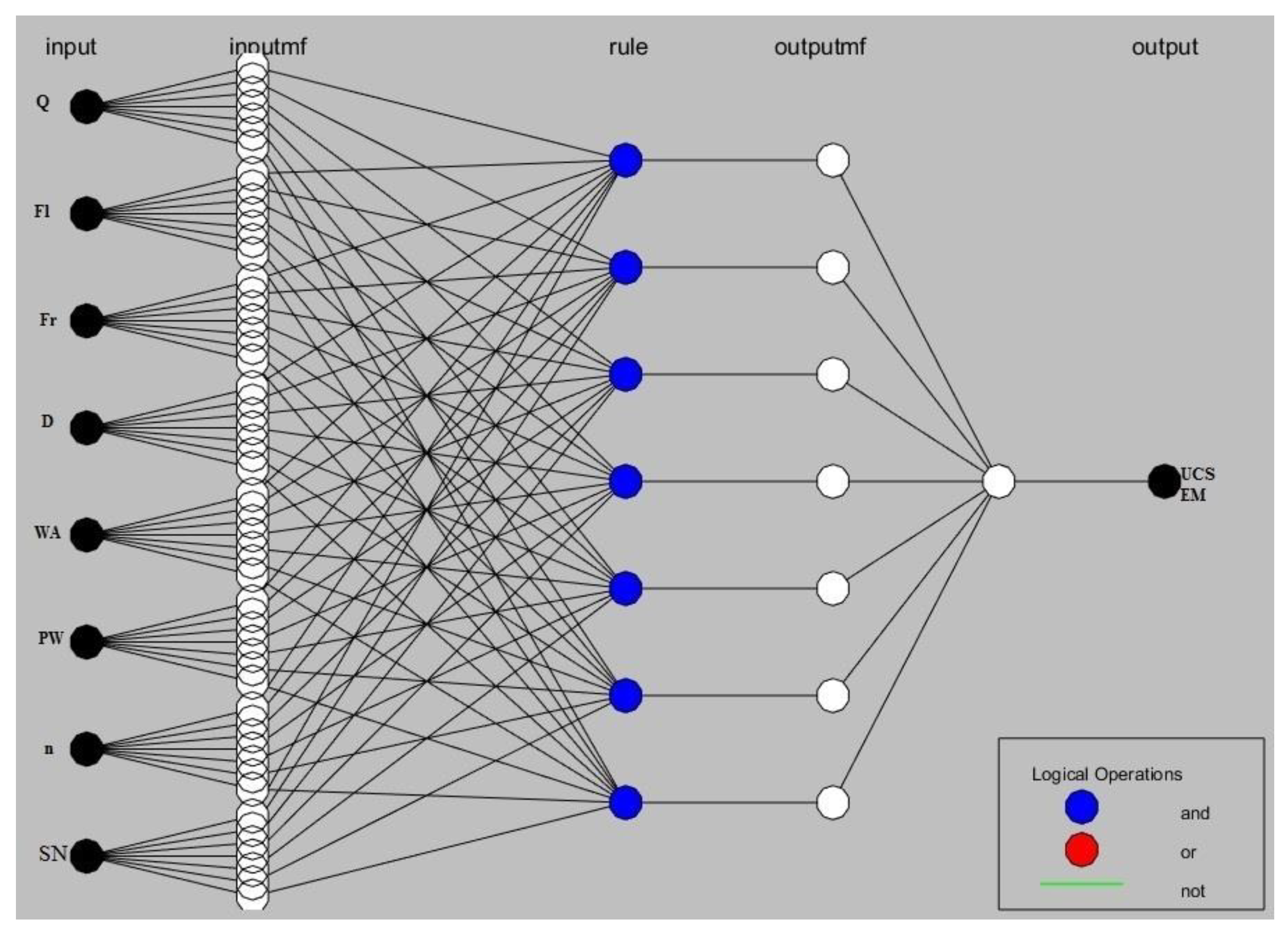
2.6. The ANFIS Method

In classical logic, each member’s membership function (MF) is 0 if it is not in the set and 1 if it is in the set [49]. Conversely, each member of the fuzzy set can have an MF value between 1 and 0, which is expressed in the form of Equation (20) according to the mathematical rules:

$$A=\left\{x,;{\mu }_A(\mathrm{x})\right\}\left|x\in \mathrm{x}\right|$$

(20)

The MF degree indicates the level value of dependence of the member on the fuzzy set. Several fuzzy inference systems (FIS) have been presented. Two types of FIS, such as the Sugeno and Mamdani algorithms, are commonly used. The difference between the two methods is due to the fuzzy rules used. The FIS is displayed as a basic rule system made up of a set of linguistic rules that can show any system with high accuracy and act like a general-purpose forecaster. The rule systems based on fuzzy logic theory use linguistic parameters, including results and rules. Rules are represented as inference or non-equality. Fuzzy-based rule systems are if and then base signified via the if rule and then the result. To demonstrate the capabilities of both neural networks and fuzzy systems, neuro-fuzzy systems (NFS) can be introduced. One of the NFS that allows fuzzy systems to learn rules with a BP (back-propagation) algorithm is the ANFIS [17]. The final FIS output is a simplification of the given average bias of each output rule. Using Sugeno FIS, here is a grouping of x and y inputs. For example, the output f is expressed by two fuzzy rules [17]:

$$\begin{array}{l}{\mathrm{Rule} 1: \mathrm{If} \mathrm{X} \mathrm{is} \mathrm{A}}_1{ \mathrm{and} \mathrm{Y} \mathrm{is} \mathrm{B}}_1{ \mathrm{then} \mathrm{F}}_1{=\mathrm{P}}_1{\mathrm{X}+\mathrm{Q}}_1{\mathrm{Y}+\mathrm{R}}_1\\ {\mathrm{Rule} 2: \mathrm{If} \mathrm{X} \mathrm{is} \mathrm{A}}_2{ \mathrm{and} \mathrm{Y} \mathrm{is} \mathrm{B}}_2{ \mathrm{then} \mathrm{F}}_2{=\mathrm{P}}_2{\mathrm{X}+\mathrm{Q}}_2{\mathrm{Y}+\mathrm{R}}_2\end{array}$$

(21)

In the ANFIS method, the variables were divided into two categories: testing and training, with 25% and 75% of the whole data, respectively. In order to train the ANFIS model, the combined method (a combination of recursive error propagation with the least squares) was used.

2.7. KNN Approach

The KNN is a learning algorithm that has been studied in the pattern recognition method for several decades [11]. Studies suggest that the KNN and support vector machine (SVM) perform better than other methods, such as a linear approximation of the smallest squares, naïve Bayes, and neural networks [11]. In the KNN method, it is assumed that there is training data for categorization, that the KNN algorithm has become similar among the pre-categorized training data based on a criterion, and that the KNN classes are used to predict the experimental data category by scoring the data of each selected category. If more than one neighbor belongs to the same category, their total score is used as the weight of that class, and the class with the maximum score is allocated to the test data. If it exceeds a threshold value, more than one class can be allocated to the test data. One problem with this method is the determination of the K value, and to determine it, sequences of tests with various K values must be performed to obtain the best value of K. Another disadvantage of KNN is the computational time complexity required to navigate all educational data [11]. The theory of the KNN method is summarized below.

• Select the optimal K value;
• Obtain the distances based on input specifications;
• Form the K class according to the closest distance (maximum similarity) and then calculate the distance of the new record from all educational records;
• Choose the nearest neighbor;
• Use the K category label of the nearest neighbor to predict the new record category.

2.8. Evaluating Criteria

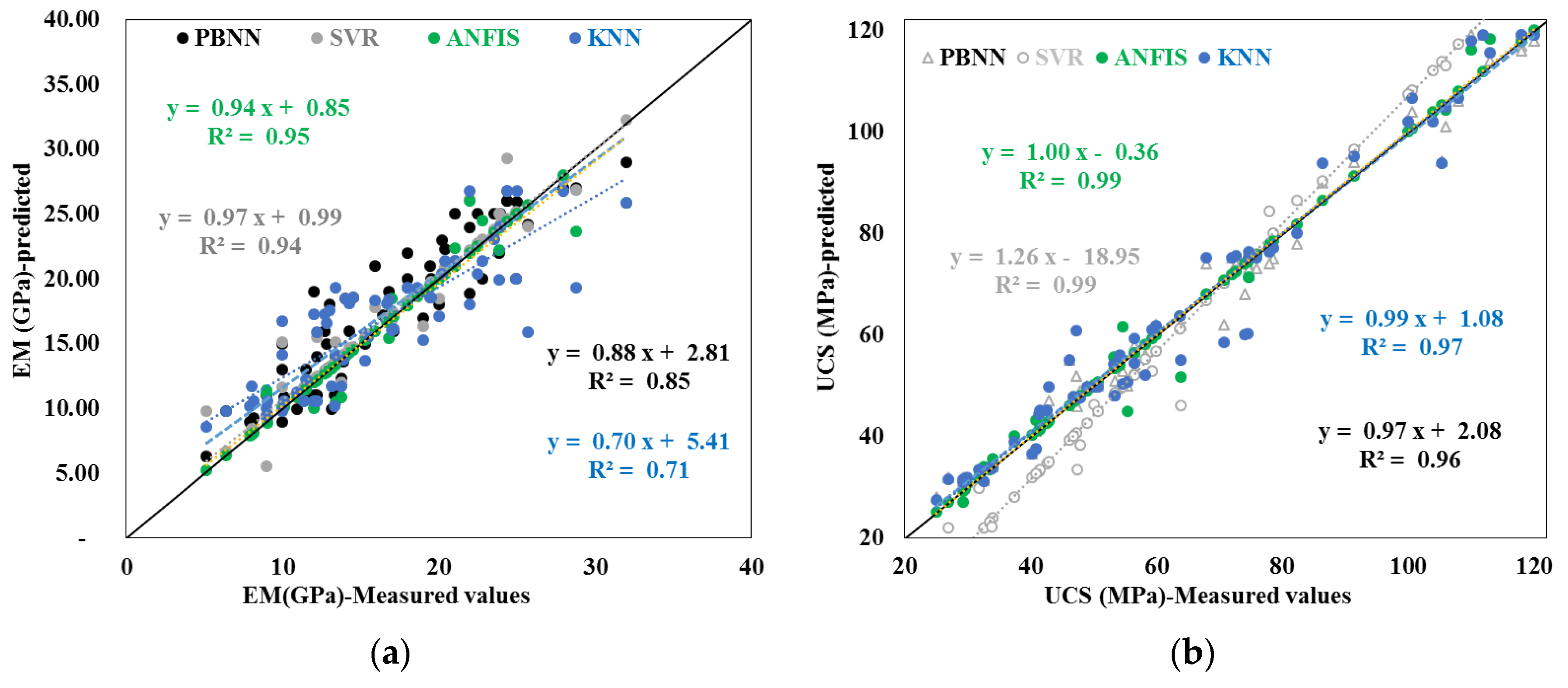
The determination coefficient (R²), mean absolute percentage error (MAPE), the variance accounted for (VAF), and root mean square error (RMSE) are used for appraising the performance of the empirical relationships [50,51,52]. The proposed relationship performs better: when R² is one, VAF is 100 and MAPE and RMSE are close to zero.

$$\mathrm{RMSE}=\sqrt{\frac{1}{N}{\displaystyle \sum _{i=1}^N{(y-y^{\prime })}^2}}$$

(22)

$$\mathrm{VAF}\%=\left[1-\frac{\mathrm{Variance} (\mathrm{y} - {\mathrm{y}}^{\prime })}{\mathrm{Variance} \left(\mathrm{y}\right)}\right] \times 100$$

(23)

$$\mathrm{MAPE}\%=\frac{1}{\mathrm{N}}{\displaystyle \sum _{i=1}^N\left|\frac{(\mathrm{y}-{\mathrm{y}}^{\prime })}{y}\right|}\times 100$$

(24)

where n is the total data, y is the actual value of the UCS or EM, $y^{·}$ is the predicted UCS or EM using the model, and $\overline{y}$ is the average of the real values.

3. Results

3.1. Laboratory Results

The texture of the samples was detrital or granular, and they were immature to sub-mature. The specimens were categorized as litharenite and feldspathic litharenite in the nature of folk classification [53]. Meta quartz was the most plentiful mineral in the samples, in sizes of medium to slightly fine sand with poor sorting and rounding. Chert, phosphate fragments, phosphate-lime, and very fine crystalline pieces form rock fragments, and muscovite, plagioclase, orthosis, and iron oxide were also presented in the samples. The types of cement were carbonate and iron oxide, and the matrix was silty. The secondary minerals include turbid minerals, such as iron oxides. Silt forms the sample matrix, and carbonate and iron oxides are the cement of the specimens.

According to the Anon [54] classification, the specimens with a mean of PW = 4.20 km/s were classified in the high wave velocity category (

Table 2. Measured properties on the samples.

	Q (%)	Fl (%)	Fr (%)	D (g/cm3)	UCS (MPa)	EM (GPa)	WA (%)	PW (km/s)	n (%)	SN (MPa)
Mean	11.15	38.04	48.66	2.58	63.87	16.41	4.05	4.20	6.56	37
Standard Error	0.24	0.36	0.65	0.02	3.41	0.76	0.33	0.06	0.56	0.79
Standard Deviation	1.95	2.85	5.18	0.13	27.31	6.10	2.66	0.50	4.47	6.35
Variance	3.79	8.12	26.82	0.02	745.60	37.22	7.09	0.25	20.01	40.32
Kurtosis	(0.43)	(0.09)	(0.24)	0.33	(0.74)	(0.58)	(1.05)	(0.38)	(1.25)	(0.74)
Skewness	0.14	0.31	(0.12)	(0.85)	0.59	0.38	0.35	(0.14)	0.06	0.59
Minimum	7.00	31.32	37.38	2.20	25.10	5.13	0.08	3.00	0.10	28
Maximum	15.24	44.80	59.60	2.79	120.00	32.00	9.50	5.10	14.25	50
Samples number	64.00	64.00	64.00	64.00	64.00	64.00	64.00	64.00	64.00	64.00

). According to the Schmidt hardness number test, the average hardness of the studied samples equals 37. The mean porosity of the samples is 6.56%. Additionally, the specimens were classified in a fairly low porosity class [54]. The density of the samples was 2.58 g/cm³ (Table 2). Hence, the studied samples were categorized into high-density classes [54]. The average UCS of the samples was 63.87 MPa. Therefore, based on Deere and Miller’s classification [55], the assessed samples were categorized as a weak class in terms of strength.

The results showed that the percentage of problematic minerals, such as clays, in the samples was negligible. High-surface clay minerals absorb water and reduce strength [56,57,58]. Some samples, which contained a large amount of silty matrix, had lower strength. Additionally, samples with carbonate cement showed less resistance than the samples with iron oxide cement. The results also show that the static properties of the sandstones are directly proportional to the percentage of SiO₂ and inversely proportional to the amount of Al₂O₃. The effect of petrological characteristics on the static features of rocks has been investigated by different researchers, and similar outcomes were stated. In general, the strength of sandstones depends on various factors, including physical, mineralogical, and textural properties, and their mineralogical importance is of great importance due to their involvement in the formation of secondary structures [26,59,60].

Harder minerals, such as quartz and feldspar, can make the rock more resistant to abrasion and deformation [61,62]. Clay minerals can have a significant effect on the mechanical properties of rocks [63]. The presence of clay minerals can affect a number of important rock properties, including strength, deformation, permeability, and shear behavior [64]. One of the main ways in which clay minerals affect rock mechanical properties is by influencing the degree of cementation and porosity of the rock [65,66]. Clay minerals can act as a binding agent, helping to hold sediment grains together and increase the strength of the rock [67,68]. However, if too much clay is present, it can reduce the porosity of the rock and make it less permeable [69,70].

The effects of the physical and mineralogical properties of the samples on static properties (UCS and EM) using simple and multivariate regression methods have been further investigated in detail.

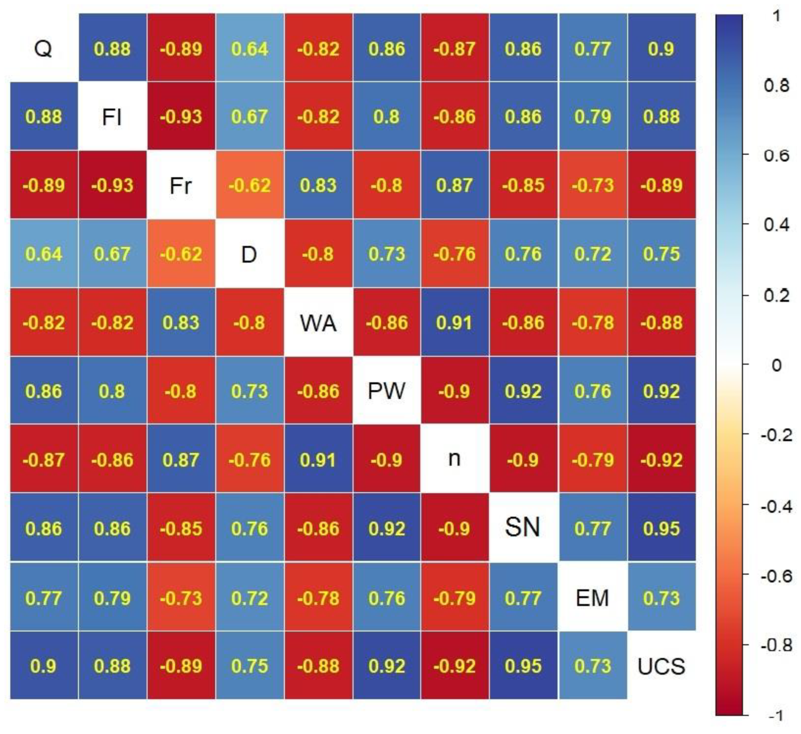
3.2. Correlation Heatmaps and Simple Regression Analysis

The correlation matrix of the variables is presented in Figure 2. The results show that the quartz and feldspar percentages have a positive effect on the static properties. In contrast, the percentage of fragments has a negative impact on the UCS and EM. It is observed that the Schmidt hardness number and porosity have the greatest effect on the UCS and EM, respectively. Abdi and Khanlari [33] stated that wave velocity has the greatest effect on the UCS. Porosity% is a suitable variable to estimate the strength of rocks [9]. In this study, porosity can also be usable for forecasting the UCS and EM. A high correlation of density, PW [10], and porosity [37] with the UCS has been reported.

Various criteria were used to evaluate the relationships (

Table 3. Simple regression results.

Regression Equation	%R2	DW	RMSE	VAF%	Equation No.
UCS = −0.02 + 19.06 SN	89.75	1.50	6.25	88.95	(25)
UCS = 100.88 − 5.642 n	85.43	1.57	6.95	84.69	(26)
UCS = −148.8 + 50.69 PW	84.80	1.5	8.89	84.01	(27)
UCS = 100.20 − 8.976 WA	76.62	1.52	10.56	75.02	(28)
UCS = −330.9 + 152.9 D	55.80	1.5	18.96	54.69	(29)
UCS = 291.8 − 4.685 Fr	78.97	1.89	9.2	78.32	(30)
UCS = −255.6 + 8.397 Fl	76.78	1.90	10.11	75.39	(31)
UCS = −76.50 + 12.592 Q	80.54	2.10	8.12	80.12	(32)
EM = −10.59 + 2.422 Q	59.71	1.51	16.03	58.62	(33)
EM = 58.30 − 0.861 Fr	62.33	1.29	14.39	62.30	(34)
EM = −47.90 + 1.691 Fl	53.38	1.34	26.35	52.6	(35)
EM = 4.75 + 2.202 SN	59.96	1.5	15.90	58.95	(36)
EM = 23.518 − 1.083 n	63.02	1.35	13.02	62.85	(37)
EM = −22.99 + 9.39 PW	58.31	1.60	17.62	57.39	(38)
EM = 23.643 − 1.786 WA	60.75	1.51	14.36	59.86	(39)
EM = −68.5 + 32.91 D	51.77	1.52	28.36	50.29	(40)

) and are identified by Equations (25)–(40). When the coefficient of determination and VAF are 100%, and the error is 0%, the presented relationship has the maximum efficiency. In order to check the independence of errors of the developed equations, the Durbin–Watson (DW) values were assessed. The value of this index must be between 1.5 and 2.5 [71]. In this study, this statistic shows that there is no problem with using the proposed relationships (Table 3).

3.3. UCS and EM Estimation Using Multiple Linear Regression Method

The multiple linear regression analysis approaches have been extensively used to estimate the geo-mechanical characteristics [35,72]. This method was performed by a simultaneous method. In simultaneous regression, input variables are entered into the equation at the same time, and each predictor variable is evaluated like the other independent variables entered. The estimation of the static properties of sandstones is in the form of Equations (41)–(54) (

Table 4. Developed regression equations to estimate static properties.

Class of Inputs	Equation	R2%	DW	Equation No.
Petrography, physical and mechanical	UCS = 25.7 + 1.58 Q − 0.44 Fl − 1.18 Fr + 11.90 D + 0.41 WA + 10.19 PW − 0.92n + 8.9 SN	93.18	1.59	(41)
	EM = −75.6 + 0.81 Q + 1.07 Fl + 0.41 Fr + 9.16 D−0.29 WA + 0.57 PW − 0.22 n − 7.11 SN	72.21	1.34	(42)
Petrography and physical	UCS = 7.0 + 3.76 Q + 0.24 Fl − 1.04 Fr + 27.9 D − 0.22 WA − 2.28 n	90.44	1.65	(43)
	EM = −73.9 + 9.07 D − 0.31 WA − 0.24 n + 0.84 Q + 1.06 Fl + 0.42 Fr	72.19	1.63	(44)
Petrography and mechanical	UCS = 29.3 + 13.31 PW + 5.61 SN + 1.62 Q − 0.202 Fl − 1.261 Fr	93.77	1.58	(45)
	EM = −71.3 + 2.65 PW + 0.397 SN + 0.745 Q + 1.257 Fl + 0.37 Fr	68.65	1.52	(46)
Mechanical and physical	EM = −11.0 + 1.17 PW + 0.408 SN + 9.41 D − 0.318 WA − 0.41 n	67.51	1.50	(47)
	UCS = 5.9 + 9.73 PW + 6.37 SN − 1.5 D − 0.216 WA − 1.833 n	92.79	1.63	(48)
Petrography	EM = −72.4 + 1.382 Q + 1.469 Fl + 0.359 Fr	65.93	1.65	(49)
	UCS = −5.7 + 6.59 Q + 1.85 Fl − 1.522 Fr	84.65	2.2	(50)
Physical	UCS = 59.4 + 15.4 D − 1.39 WA − 4.535 n	86.20	1.52	(51)
	EM = −5.4 + 10.65 D − 0.414 WA − 0.617 n	66.72	1.54	(52)
Mechanical	UCS = −53.3 + 17.37 PW + 8.35 SN	91.24	1.56	(53)
	EM = −7.74 + 4.07PW + 1.334 SN	61.06	1.53	(54)

). In this study, the effect of various classes, including petrography (quartz%, feldspar%, and fragments %), physical (water absorption (WA), porosity (n), and density (D)), and mechanical (PW and SN) properties as inputs on the UCS and EM were assessed. It is observed that the effect of the inputs on the UCS is more than the EM. Additionally, the mechanical class has the lowest effect on the EM compared with other classes.

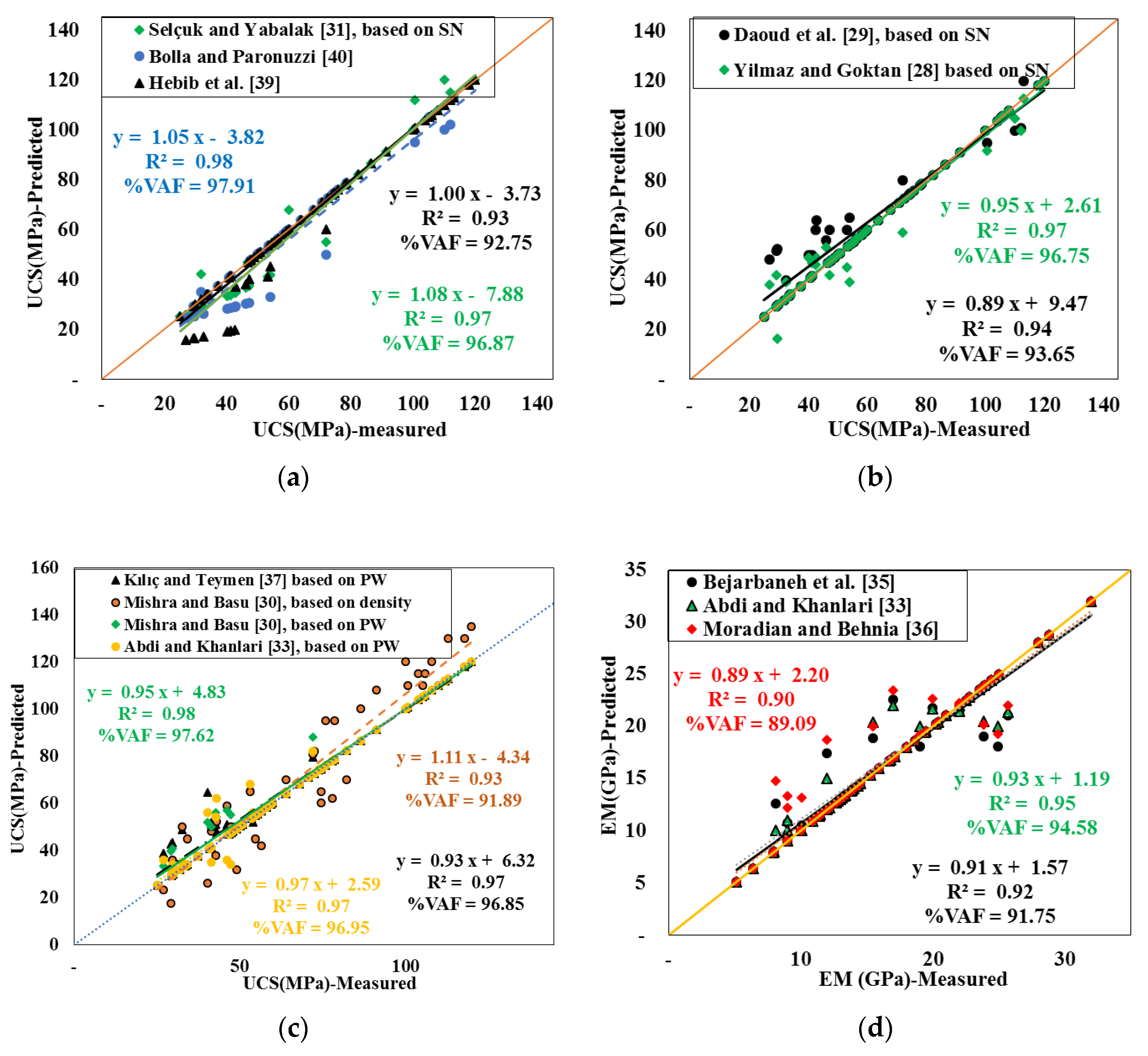
3.4. Comparison with Previous Studies

Many relationships between the physical and mechanical characteristics of sandstone rocks with non-destructive properties were proposed by other scholars (Table 1); however, it is not clear how valid their results are for Iranian formations. Therefore, here, the efficiency of the existing relationships using VAF and R² based on the measured data of the PW, density, Schmidt hardness number, porosity, and mechanical characteristics of the samples of the dam sites were evaluated, and the most accurate relationship was identified. To do this, the UCS and EM were calculated using previous empirical relationships. Then, the relationships between the predicted UCS and EM and measured UCS and EM were assessed. Assessing the relationships of Abdi and Khanlari [30], Kılıç and Teymen [33], and Mishra and Basu [27] to estimate the UCS of the studied sandstones shows that these relationships are used to estimate the UCS with acceptable accuracy (Figure 3). Additionally, the measured UCS and EM values were compared with the results of Selcuk and Yabalak [28], Bolla and Paronuzzi [36], Hebib et al. [35], Daoud et al. [26], and Yilmaz and Goktan’s [25] relationships (Figure 3). Based on the mentioned relations, the best correlation between these values is related to the linear relationship (Figure 3). The relationship between Bolla and Paronuzzi [36] is more accurate than other relationships. This experimental relationship shows a high correlation between the SN and UCS. Abdi and Khanlari [30], Bejarbaneh et al. [13], and Moradi and Behnia [32] proposed several empirical relationships for estimating the EM. Figure 3 shows that the relationships between measured and predicted EM have a high correlation. Based on VAF% and the coefficient of determination, Abdi and Khanlari’s [30] relationship has the highest accuracy compared to the other relationships because of the lithological similarity of the samples in both studies. The sandstones of the present study and Abdi and Khanlari [30] were classified as feldspathic litharenite and litharenite types.

3.5. The SVR Results

The SVR modeling was performed by coding in MATLAB (Version 2021) software. The percentage of test and train data for constructing the SVR model and optimum values of the kernel of radial basis function parameters, such as ε, γ, and C, for predicting the static properties are presented in

Table 5. Parameters of the developed SVR model to estimate UCS and EM.

	UCS	EM
Train data	75% of whole data	75% of whole data
Test data	25% of whole data	25% of whole data
Epsilon	0.0022	0.0016
C	35	26
Gamma	0.90	0.40

. In this research, the radial basis kernel function has been used for the training and testing of data by the SVR method. Other researchers have reported the high performance of this function in estimating the mechanical properties of the rocks [16,17,20,48].

The error values and laboratory value correlations with estimated mechanical properties by the SVR technique for various datasets are revealed in Figure 4 and Figure 5.

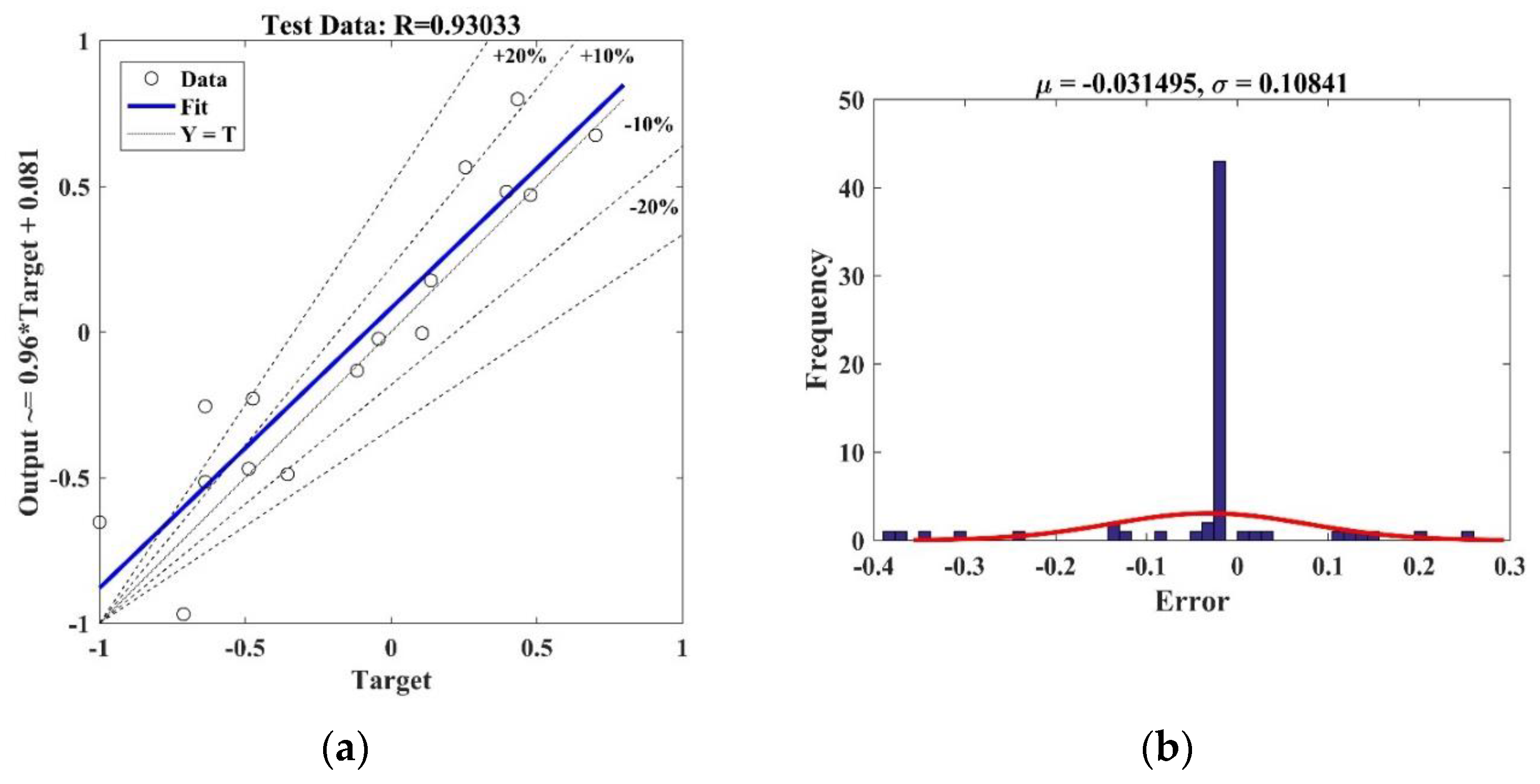
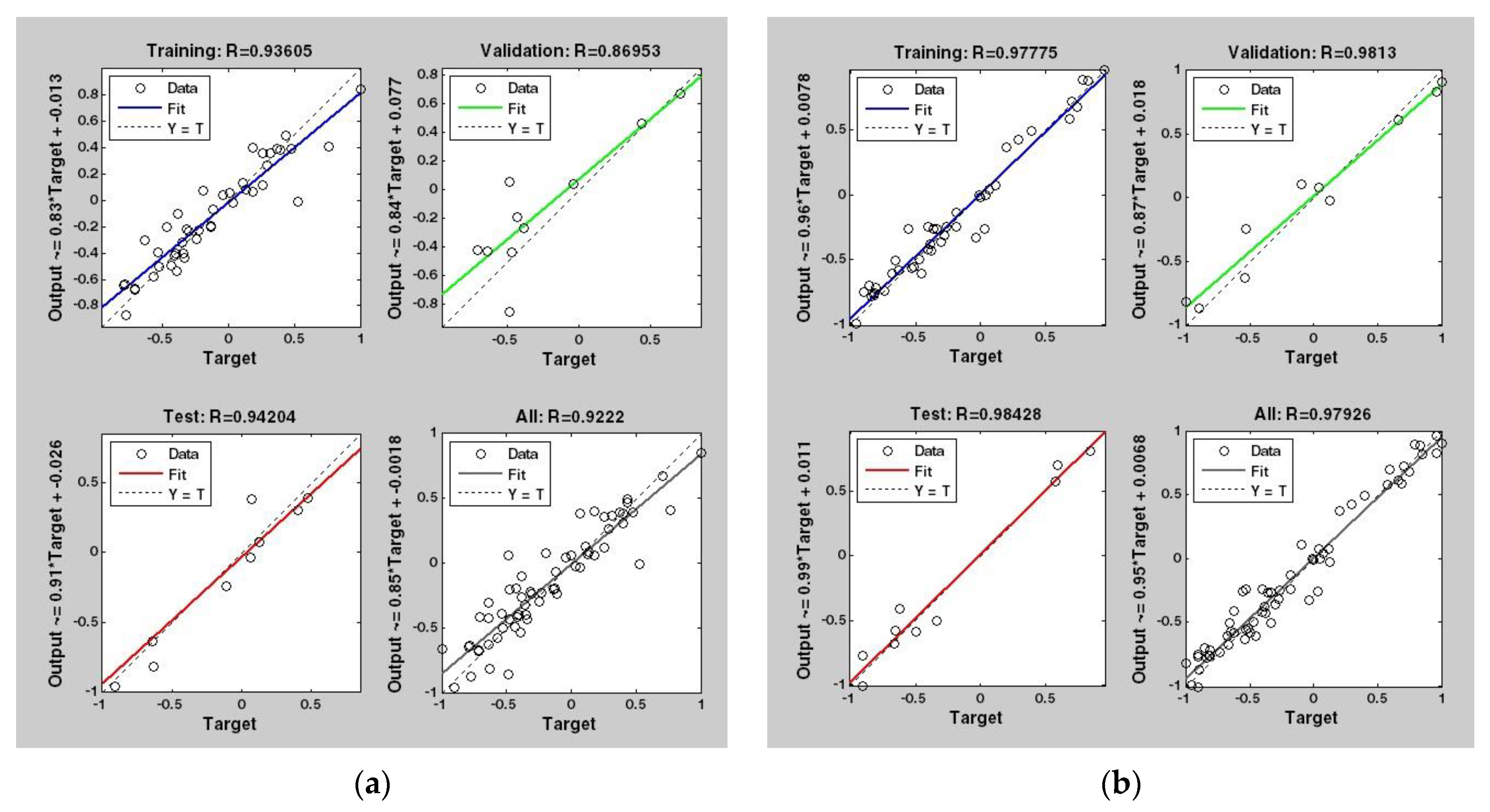
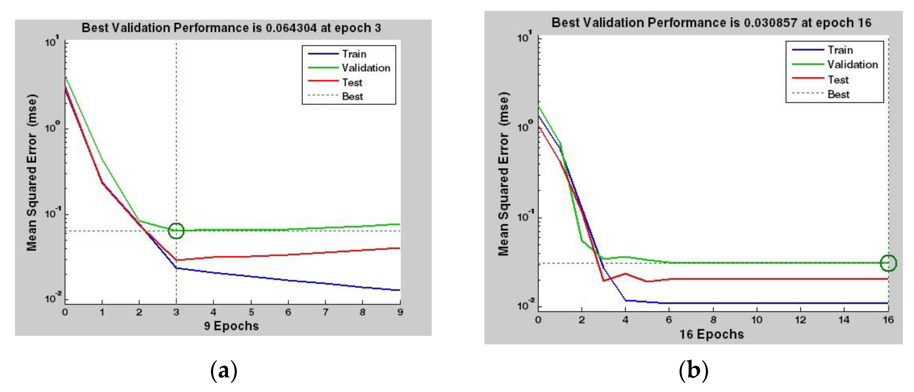
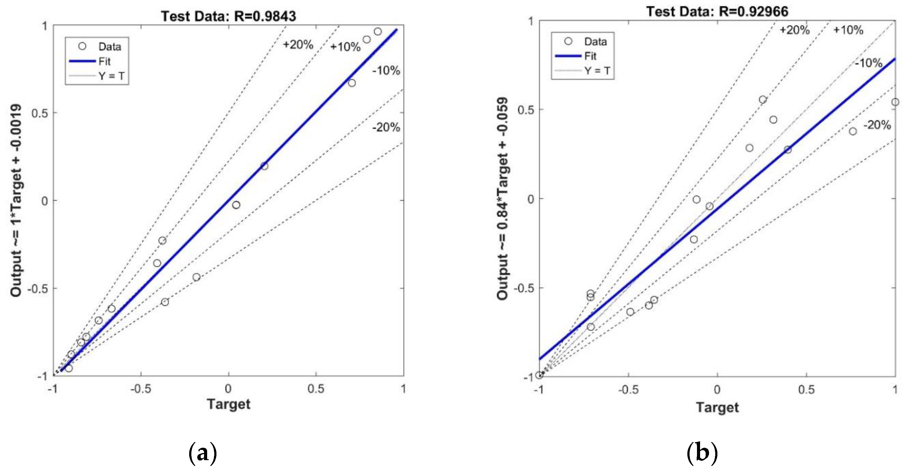
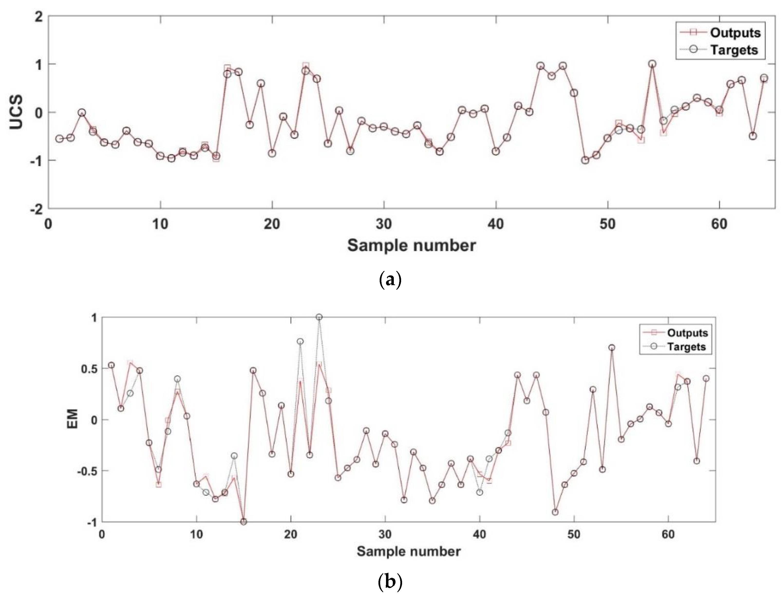
3.6. Estimation of UCS and EM Using BPNN

Using the BPNN, a multilayer feed-forward neural network is presented. In this type of network, the direction of information flow moves from the input layers to the output layers [8,73,74]. Using the Neural Net Fitting Toolbox to check the performance of various training algorithms, such as the LM (Levenberg–Marquardt), BR (Bayesian regularization), and SCG (Scaled Conjugate Gradient) to estimate the dependent variables, several combinations with a different number of neurons (for different training algorithms), using a trial and error process, were applied to a hidden layer. The LM algorithm showed the best results for forecasting the UCS and EM. The ideal obtained BPNN contains four neurons in a hidden layer with eight inputs, such as quartz%, feldspar%, fragments%, the Schmidt hardness number, density, water absorption%, porosity%, and PW as well as two outputs, including the UCS and EM (

Table 6. BPNN results using LM, BR, and SCG training functions.

Optimum BPNN	Activation Functions	Training Functions	R% (for Test Data)		RMSE (for Test Data)
			UCS	EM	UCS	EM
8*4*2	{tansig, Purlin}	LM	98.43	94.20	0.17	0.24
8*4*2	{tansig, Purlin}	SCG	97.25	93.19	0.18	0.26
8*5*2	{tansig, Purlin}	BR	97.01	93.00	0.19	0.28

and Figure 6 and Figure 7). All data in the present study were divided into three groups:

• The train set, with 70% of the total data for training the network;
• The test group, with 15% of the total data to test the network;
• The validation set, with 15% of the total data for preventing overfitting.

The results showed that the fourth neuron is the most suitable for forecasting the UCS and EM. By comparing the BPNN results with multiple linear models, the BPNN is more precise than MRA for forecasting the UCS and EM. Similar outcomes were suggested by previous researchers [8,10].

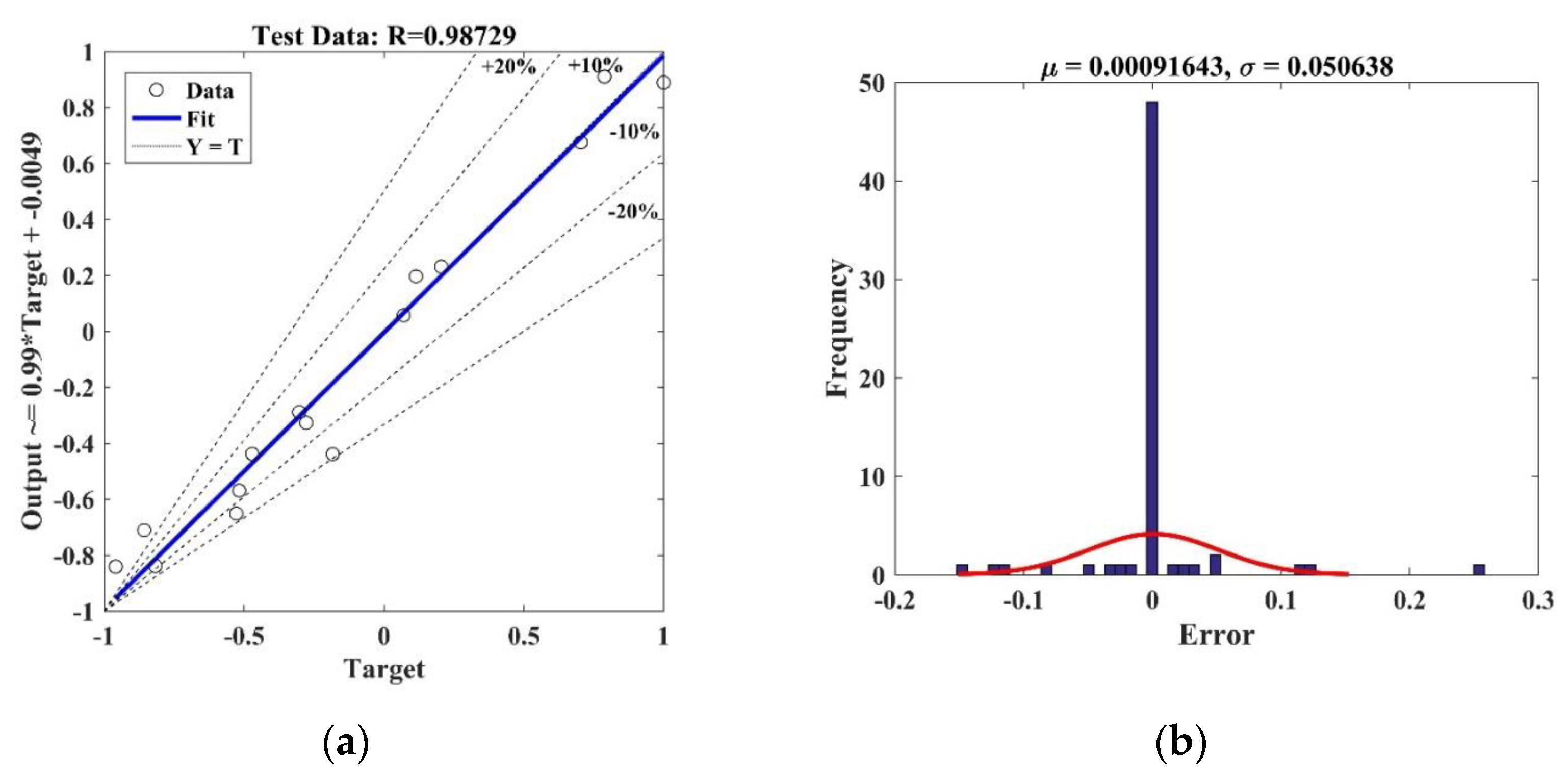
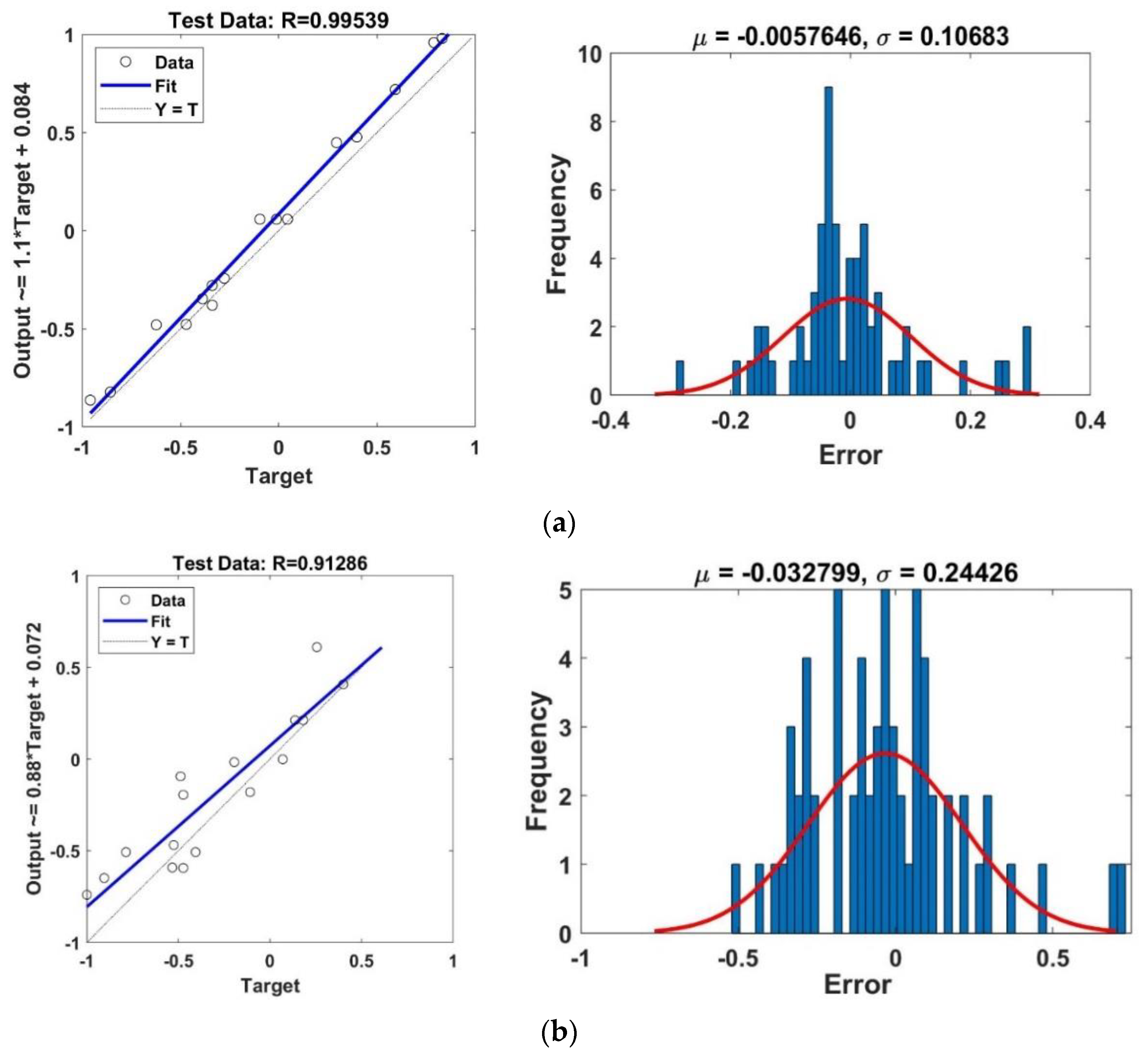
3.7. Results of ANFIS Approach

In accordance with the other assessed intelligent methods, the input data for modeling using the ANFIS include the Schmidt hardness number (SN), compressional wave velocity (PW), water absorption (WA), porosity (n), and density (D), where the UCS and EM are outputs of 64 samples (Figure 8). In the ANFIS method, by coding in MATLAB (Version 2021) software, the MFs of the input data for each of the parameters are 7 (

Table 7. Used ANFIS model components.

Parameters	EM	UCS
Train data	75%	75%
Test data	25%	25%
FIS Generation approach	Genfis2	Genfis2
Influence radius	0.58	0.62
Number of epochs	1500	1200
Error goal	0	0
Type	Sugeno	Sugeno
Rules	7	7
Number of MFs	7	7
Input MF type	GM	GM
Output MF type	Linear	Linear

). In the Inputmf (i.e., input membership function) layer, inputs move across MFs. The MFs of each function can be a suitable parameter. The Gaussian membership (GM) function was selected in the current research. The MFs degree shows the level of the member’s membership to the fuzzy set.

The ANFIS model components developed in this study are summarized in Table 7 and Figure 9 and Figure 10.

Figure 9 and Figure 10 show the results of the ANFIS model for the test datasets. As can be seen, the ANFIS method shows higher accuracy than the SVR method. The error value using the ANFIS models is presented in Figure 10.

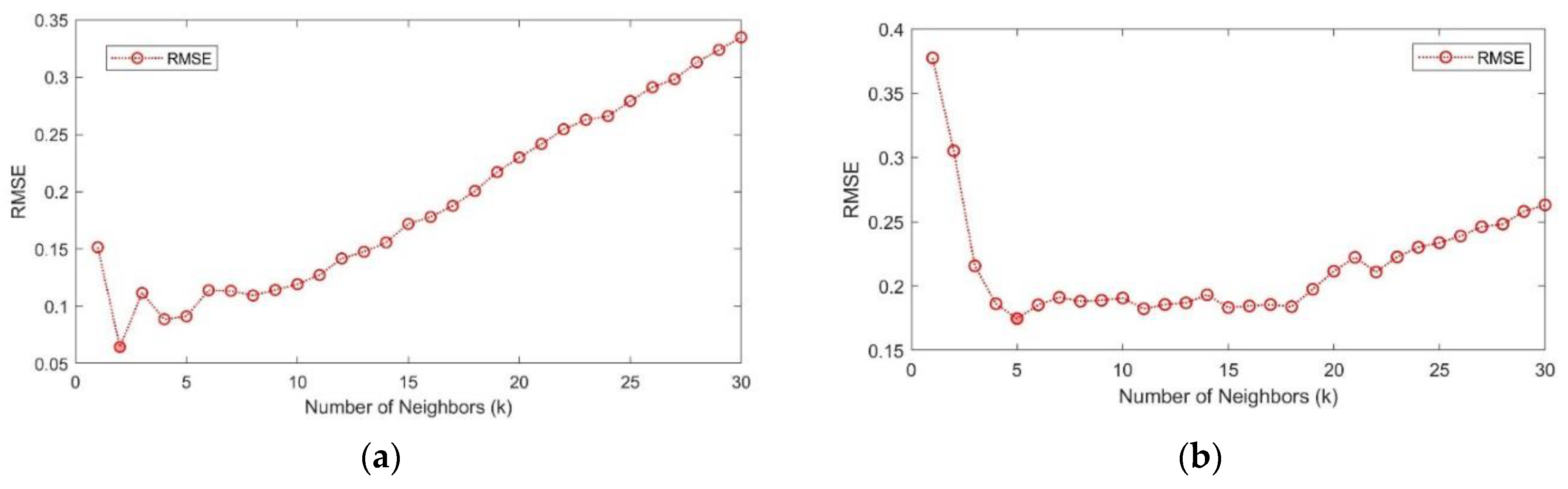
3.8. The KNN Results

In order to apply the KNN method to the data and to also determine the best K value, the coding of the KNN algorithm was written in the form of a program in MATLAB (Version 2021), which was run 216 times for the K values, from 1 to 30 programs, and the amount of error was then measured. Similar to SVR and the ANFIS, 75% and 25% of the total data were used to train and test the models. The results displayed that the lowest estimation error of the UCS and EM was obtained at K = 2 and K = 5, respectively (Figure 11). The error of this network for estimating the UCS and EM with respect to the K values is equal to 0.07 and 0.17, respectively (Figure 11). Figure 12 shows the KNN results for estimating the mechanical properties.

3.9. Nonlinear Multivariate Regression Analysis

In statistics, multivariate nonlinear regression is a type of regression analysis in which the observational data are modeled by combining nonlinear functions between independent and dependent parameters [75]. In this study, nonlinear regression between parameters is considered. In this way, firstly, between the UCS and the EM with each of the independent parameters, various types of nonlinear regression were fitted (see Equations (55)–(70)), and the best fit was selected (

Table 8. Most accurate nonlinear regression between variables.

Equation	R2	Type of Equation	Equation No.
UCS = 0.43 Fl2 − 24.30 Fl + 367.77	0.76	Polynomial	(55)
UCS = 106.91 e−0.09n	0.91	Exponential	(56)
UCS = 0.16 Fr2 − 20.50 Fr + 669.86	0.83	Polynomial	(57)
UCS = 106.43 e−0.15WA	0.83	Exponential	(58)
UCS = 484.46 D2 − 2295.24 D + 2752.06	0.71	Polynomial	(59)
UCS = 1.25 Q2 − 15.43 Q + 75.59	0.82	Polynomial	(60)
UCS = 1.84 e 0.82PW	0.89	Exponential	(61)
UCS = 0.03 SN2 − 4.60 SN + 250	0.91	Polynomial	(62)
EM = 0.06 FL2 − 3.22 Fl + 44.87	0.60	Polynomial	(63)
EM = 0.04 Fr2 − 4.61 Fr + 148.67	0.53	Polynomial	(64)
EM = 24.47 e−0.07n	0.66	Exponential	(65)
EM = 24.82 e−0.12WA	0.65	Exponential	(66)
EM = 1.10 e0.63PW	0.62	Exponential	(67)
EM = 0.19 Q2 − 1.88 Q + 12.59	0.58	Polynomial	(68)
EM = 76.45 D2 − 353.40 D + 417.94	0.59	Polynomial	(69)
EM = 0.01 SN2 − 0.20 SN + 9.42	0.59	Polynomial	(70)

). Then, the appropriate nonlinear regression was established between all independent parameters with the UCS and EM. The values of the determination coefficient are given in Table 8.

Finally, using the Gauss–Newton algorithm with 200 maximum iterations and a tolerance of 0.00001, some nonlinear multivariate regression (NLMVR) equations were developed to estimate the UCS and EM (

Table 9. Developed equations using the NLMVR method.

Developed Equations	R2	RMSE	Condition	Equation No.
EM = 0.31 Fl1.2 − 6.71 Fl + 135.15 + 24.03Exp(−0.07n) + 24.92Exp(−0.12WA) + 1.08Exp(0.63PW) + 0.13 Fr1.57 − 6.31 Fr + 148 + 0.24 Q1.95 − 2.08 Q + 13 + 106.32 D1.83 − 414.82 D + 418 + 0.01 SN2.00 − 0.20 SN + 14.2	0.78	172	For all inputs	(71)
EM = 0.30 Fl1.47 − 5.54 Fl + 67.78 + 24.08Exp(−0.07n) + 24.69Exp(−0.12WA) + 1.13Exp(0.62PW)	0.79	51	For inputs with R2 > 60%	(72)

). The NLMVR results indicate that when more influential variables (independent variables with determination coefficients above 60%) are used in estimating the EM, the accuracy of the developed model (i.e., Model in Equation (72)) is higher than when all variables (i.e., Model in Equation (71)) are used in estimating the EM.

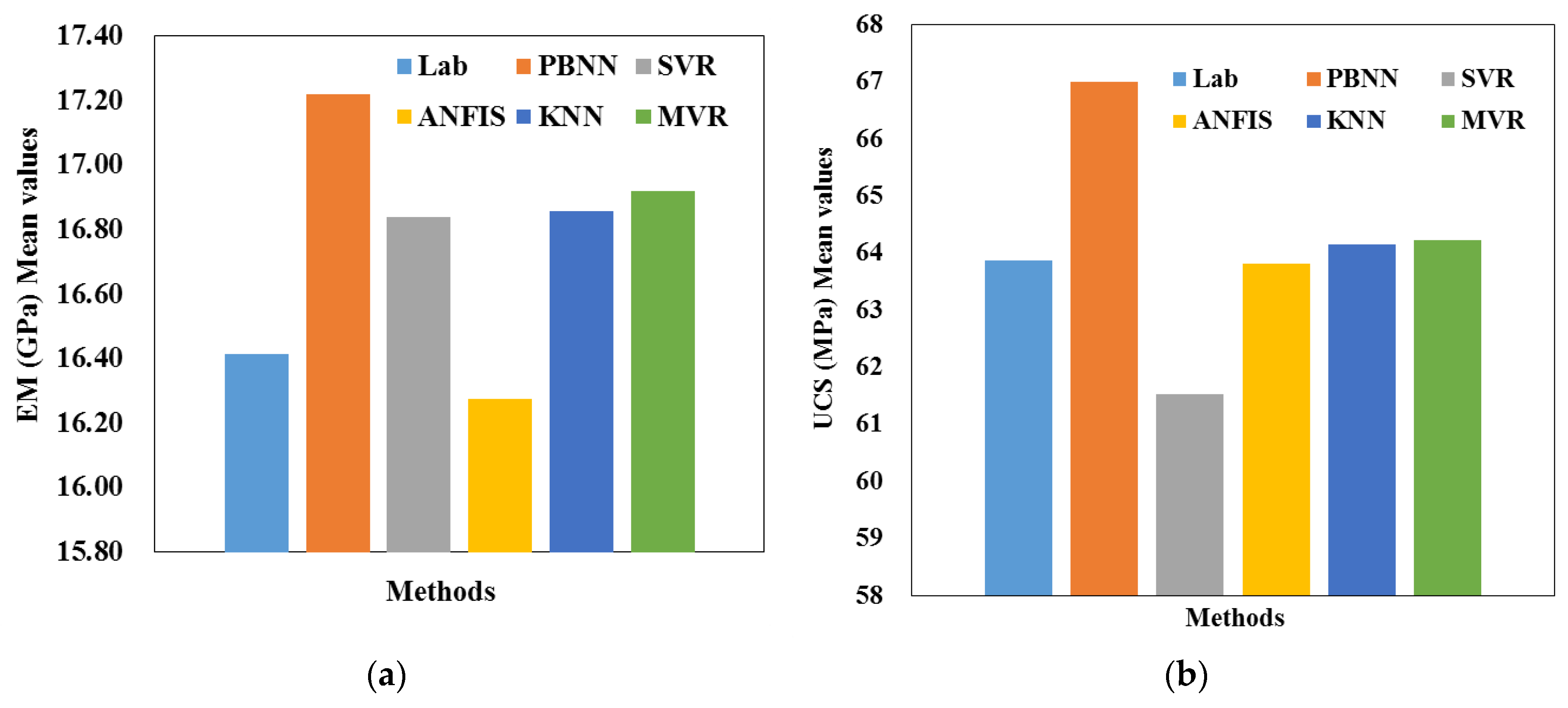
3.10. Comparison of Used Methods

Table 10. The precision of the intelligent methods used for all data.

Methods	R		MAPE%		RMSE		VAF%
	UCS	EM	UCS	EM	UCS	EM	UCS	EM
SVR	0.996	0.971	13.64	6.75	0.051	0.11	98.87	93.87
ANFIS	0.996	0.99	1.69	3.22	0.054	0.103	98.96	98.88
KNN	0.98	0.84	6.06	17.58	0.11	0.25	95.89	70.22
PBNN	0.98	0.92	5.48	5.69	0.17	0.25	95.96	84.00

and Figure 13 show the accuracy of the methods used for forecasting static properties. According to the statistical criteria (i.e., R, MAPE, RMSE, and VAF), the ANFIS method has higher accuracy than other methods. The SVR method also has very high accuracy in the UCS and EM estimations, with a slight difference after the ANFIS method. This is because SVR uses the principle of minimizing structural risk and adapting the ability of the model to existing training data [76]. The number of inputs also affects the accuracy of the methods. Considering that the number of inputs in the modeling in this research (8 inputs) is high, the ANFIS method performs with higher accuracy than the other methods [17]. Based on the correlation coefficient, all methods (R > 70%) accurately estimate the UCS and EM.

Figure 14 compares the measured values of the UCS and EM and the predicted values using the methods employed. As can be seen, the ANFIS method shows the best results for forecasting static properties. The average predicted UCS and EM from all five methods are 64.14 Mpa and 16.82 Gpa, respectively. The mean percentages of the predicted UCS and EM changes obtained from all five methods compared to the measured value are 0.42% and 2.48%, respectively, both of which show less than a 5% error, and the presented methods can predict static properties with high accuracy.

4. Conclusions

The physical and mechanical properties are the most important parameters of rocks and are widely required in civil and mining projects to study rock mechanics. On the other hand, index tests are easy and can be performed in the field or site of projects. In the current research, after the petrography studies, physical, mechanical, and dynamic experiments were performed on the sandstone samples obtained from the Lar and Siah Bisheh dam sites. The SVR, KNN, ANFIS, BPNN, and simple and multivariate regression methods were used to predict static properties, such as the uniaxial compressive strength (UCS) and modulus of elasticity (EM).

Petrographic studies displayed that the sandstone specimens are categorized as litharenite and feldspathic litharenite. The results revealed that, with an increasing silty matrix, the strength of the samples decreased. Additionally, samples with carbonate cement showed less resistance than the samples with iron oxide cement. The results also showed that the UCS and EM are directly related to the SiO₂% and inversely dependent on the Al₂O₃ amount. The statistical analysis results showed that the Schmidt hardness number (SN) and porosity have the greatest effect on the UCS and EM. The evaluation of the experimental relationships of other researchers revealed that some of these relationships are useable to predict the UCS and EM of the studied sandstones. The evaluation of the criteria of models (VAF, Durbin–Watson, RMSE, and R²) using the multivariate regression method showed the high accuracy of this method for estimating the static properties. Among the training algorithms using the BPNN method, the LM showed the best results for forecasting the UCS and EM. The ideal obtained BPNN, using a trial-and-error process, contains four neurons in a hidden layer with eight inputs. By comparing the results of the employed methods, the ANFIS with R² = 0.996 for the UCS and R² = 0.99 for the EM showed the best performance for estimating the EM and UCS.

References

1. Li, S.; Wang, Y.; Xie, X. Prediction of Uniaxial Compression Strength of Limestone Based on the Point Load Strength and SVM Model. Minerals 2021, 11, 1387. [Google Scholar] [CrossRef]
2. Ren, C.; Yu, J.; Liu, S.; Yao, W.; Zhu, Y.; Liu, X. A Plastic Strain-Induced Damage Model of Porous Rock Suitable for Different Stress Paths. Rock Mech. Rock Eng. 2022, 55, 1887–1906. [Google Scholar] [CrossRef]
3. Yu, J.; Zhu, Y.; Yao, W.; Liu, X.; Ren, C.; Cai, Y.; Tang, X. Stress Relaxation Behaviour of Marble under Cyclic Weak Disturbance and Confining Pressures. Measurement 2021, 182, 109777. [Google Scholar] [CrossRef]
4. Ulusay, R.; Tureli, K.; Ider, M.H. Prediction of engineering properties of a selected litharenite sandstone from its petrographic characteristics using correlation and multivariable statistical technique. Eng. Geol. 1994, 37, 135–157. [Google Scholar] [CrossRef]
5. Yasar, E.; Ranjith, P.G.; Perera, M.S.A. Physico-mechanical behaviour of southeastern Melbourne sedimentary rocks. Int. J. Rock Mech. Min. Sci. 2010, 47, 481–487. Available online: http://pascal-francis.inist.fr/vibad/index.php?Action=getRecordDetail&idt=22570877 (accessed on 1 April 2010). [CrossRef]
6. Jin, J.; Zhang, X.; Liu, X.; Li, Y.; Li, S. Study on Critical Slowdown Characteristics and Early Warning Model of Damage Evolution of Sandstone under Freeze-Thaw Cycles. Front. Earth Sci. 2023, 15, 18–25. [Google Scholar] [CrossRef]
7. Lawal, A.I.; Kwon, S.; Aladejare, A.E.; Oniyide, G.O. Prediction of the static and dynamic mechanical properties of sedimentary rock using soft computing methods. Geotech. Eng. 2022, 28, 313–324. [Google Scholar]
8. Armaghani, D.J.; Mamou, A.; Maraveas, C.; Roussis, P.C.; Siorikis, V.G.; Skentou, A.D.; Asteris, P.G. Predicting the unconfined compressive strength of granite using only two non-destructive test indexes. Geomech. Eng. 2021, 25, 317–330. [Google Scholar]
9. Aladejare, A.E.; Akeju, V.O.; Wang, Y. Data-driven characterization of the correlation between uniaxial compressive strength and Youngs’ modulus of rock without regression models. Transp. Geotech. 2022, 32, 100680. [Google Scholar] [CrossRef]
10. Rastegarnia, A.; Lashkaripour, G.R.; Sharifi Teshnizi, E.; Ghafoori, M. Evaluation of engineering characteristics and estimation of dynamic properties of clay-bearing rocks. Environ. Earth Sci. 2021, 80, 621. [Google Scholar] [CrossRef]
11. Mahmoodzadeh, A.; Mohammadi, M.; Ibrahim, H.H.; Abdulhamid, S.N.; Salim, S.G.; Ali, H.F.H.; Majeed, M.K. Artificial intelligence forecasting models of uniaxial compressive strength. Transp. Geotech. 2021, 27, 100499. [Google Scholar] [CrossRef]
12. Siddig, O.; Gamal, H.; Elkatatny, S.; Abdulraheem, A. Applying Different Artificial Intelligence Techniques in Dynamic Poisson’s Ratio Prediction Using Drilling Parameters. J. Energy Resour. Technol. 2022, 144, 073006. [Google Scholar] [CrossRef]
13. Zoveidavianpoor, M.; Samsuri, A.; Shadizadeh, S.R. Adaptive neuro fuzzy inference system for compressional wave velocity prediction in a carbonate reservoir. Appl. Geophys. 2013, 89, 96–107. [Google Scholar] [CrossRef]
14. Chang, C.; Mark, D.; Zoback, M.B.; Khaksar, A. Empirical relations between rock strength and physical properties in sedimentary rocks. J. Pet. Sci. Eng. 2006, 51, 223–237. [Google Scholar] [CrossRef]
15. Heidari, M.; Momeni, A.; Rafiei, B.; Khodabakhsh, S.; Torabi-Kaveh, M. Relationship between Petrographic Characteristics and the Engineering Properties of Jurassic Sandstones, Hamedan, Iran. Rock Mech. Rock Eng. 2013, 46, 1091–1101. [Google Scholar] [CrossRef]
16. Wang, Z.; Li, W.; Chen, J. Application of Various Nonlinear Models to Predict the Uniaxial Compressive Strength of Weakly Cemented Jurassic Rocks. Nat. Resour. Res. 2022, 31, 371–384. [Google Scholar] [CrossRef]
17. Shahani, N.M.; Zheng, X.; Liu, C.; Li, P.; Hassan, F.U. Application of Soft Computing Methods to Estimate Uniaxial Compressive Strength and Elastic Modulus of Soft Sedimentary Rocks. Arab. J. Geosci. 2022, 15, 384. [Google Scholar] [CrossRef]
18. Cemiloglu, A.; Zhu, L.; Arslan, S.; Xu, J.; Yuan, X.; Azarafza, M.; Derakhshani, R. Support Vector Machine (SVM) Application for Uniaxial Compression Strength (UCS) Prediction: A Case Study for Maragheh Limestone. Appl. Sci. 2023, 13, 2217. [Google Scholar] [CrossRef]
19. Abdelhedi, M.; Jabbar, R.; Said, A.B.; Fetais, N.; Abbes, C. Machine Learning for Prediction of the Uniaxial Compressive Strength within Carbonate Rocks. Earth Sci. Inform. 2023, 7, 1–15. [Google Scholar] [CrossRef]
20. Asare, E.N.; Affam, M.; Ziggah, Y.Y. A Hybrid Intelligent Prediction Model of Autoencoder Neural Network and Multivariate Adaptive Regression Spline for Uniaxial Compressive Strength of Rocks. Model. Earth. Syst. Environ. 2023, 6, 1–17. [Google Scholar] [CrossRef]
21. Wang, Y.; Rezaei, M.; Abdullah, R.A.; Hasanipanah, M. Developing Two Hybrid Algorithms for Predicting the Elastic Modulus of Intact Rocks. Sustainability 2023, 15, 4230. [Google Scholar] [CrossRef]
22. Zhao, R.; Shi, S.; Li, S.; Guo, W.; Zhang, T.; Li, X.; Lu, J. Deep Learning for Intelligent Prediction of Rock Strength by Adopting Measurement While Drilling Data. Int. J. Geomech. 2023, 23, 04023028. [Google Scholar] [CrossRef]
23. Rahman, T.; Sarkar, K. Empirical Correlations between Uniaxial Compressive Strength and Density on the Basis of Lithology: Implications from Statistical and Machine Learning Assessments. Earth Sci. Inform. 2023, 1, 1–25. [Google Scholar] [CrossRef]
24. Weng, M.C.; Li, H.H. Relationship between the deformation characteristics and microscopic properties of sandstone explored by the bonded-particle model. Int. J. Rock Mech. Min. Sci. 2012, 56, 34–43. [Google Scholar] [CrossRef]
25. Naresh, K.T.; Shuichiro, Y.; Suresh, D. Relationships among mechanical, physical and petrographic properties of Siwalik sandstones, Central Nepal Sub-Himalayas. Eng. Geol. 2007, 90, 105–123. [Google Scholar] [CrossRef]
26. Ghobadi, M.H.; Heidari, M.; Rafiei, B.; Mousavi, S.D. Investigation of the relationship between mineralogical and physical properties of sandstones with their tensile strength. In Proceedings of the First National Conference on Geotechnical Engineering, Mashhad, Iran, 14 June 2013. Article COI Code: GEOTEC01_371 (In Persian). [Google Scholar]
27. Qi, Y.; Ju, Y.; Yu, K.; Meng, S.; Qiao, P. The effect of grain size, porosity and mineralogy on the compressive strength of tight sandstones: A case study from the eastern Ordos Basin, China. J. Pet. Sci. Eng. 2022, 208, 109461. [Google Scholar] [CrossRef]
28. Yilmaz, N.G.; Goktan, R.M. Comparison and combination of two NDT methods with implications for compressive strength evaluation of selected masonry and building stones. Bull. Eng. Geol. Environ. 2019, 78, 4493–4503. [Google Scholar] [CrossRef]
29. Daoud, H.S.D.; Rashed, K.A.R.; Alshkane, Y.M.A. Correlations of uniaxial compressive strength and modulus of elasticity with point load strength index, pulse velocity and dry density of limestone and sandstone rocks in Sulaimani Governorate, Kurdistan Region, Iraq. J. Zankoy Sulaimani-A 2018, 19, 57–72. [Google Scholar] [CrossRef]
30. Mishra, D.A.; Basu, A. Estimation of uniaxial compressive strength of rock materials by index tests using regression analysis and fuzzy inference system. Eng. Geol. 2013, 160, 54–68. [Google Scholar] [CrossRef]
31. Selçuk, L.; Yabalak, E. Evaluation of the ratio between uniaxial compressive strength and Schmidt hammer rebound number and its effectiveness in predicting rock strength. Nondestruct. Test. Eval. 2015, 30, 1–12. [Google Scholar] [CrossRef]
32. Armaghani, D.J.; Amin, M.F.M.; Yagiz, S.; Faradonbeh, R.S.; Abdullah, R.A. Prediction of the uniaxial compressive strength of sandstone using various modeling techniques. Int. J. Rock. Mech. Min. 2016, 85, 174–186. [Google Scholar] [CrossRef]
33. Abdi, Y.; Khanlari, G.R. Estimation of mechanical properties of sandstones using P-wave velocity and Schmidt hardness. New Find. Appl. Geol. 2019, 13, 33–47. [Google Scholar]
34. Eremin, M. Three-dimensional finite-difference analysis of deformation and failure of weak porous sandstones subjected to uniaxial compression. Int. J. Rock Mech. Min. Sci. 2020, 133, 104412. [Google Scholar] [CrossRef]
35. Bejarbaneh, B.Y.; Bejarbaneh, E.Y.; Amin, M.F.M.; Fahimifar, A.; Jahed Armaghani, D.; Majid, M.Z.A. Intelligent modelling of sandstone deformation behaviour using fuzzy logic and neural network systems. Bull. Eng. Geol. Environ. 2018, 77, 345–361. [Google Scholar] [CrossRef]
36. Moradian, Z.A.; Behnia, M. Predicting the uniaxial compressive strength and static Young’s modulus of intact sedimentary rocks using the ultrasonic test. Int. J. Geomech. 2009, 9, 14–19. [Google Scholar] [CrossRef]
37. Kılıç, A.; Teymen, A. Determination of mechanical properties of rocks using simple methods. Bull. Eng. Geol. Environ. 2008, 67, 237. [Google Scholar] [CrossRef]
38. Çobanoğlu, İ.; Çelik, S.B. Estimation of uniaxial compressive strength from point load strength, Schmidt hardness and P-wave velocity. Bull. Eng. Geol. Environ. 2008, 67, 491–498. [Google Scholar] [CrossRef]
39. Hebib, R.; Belhai, D.; Alloul, B. Estimation of uniaxial compressive strength of North Algeria sedimentary rocks using density, porosity, and Schmidt hardness. Arab. J. Geosci. 2017, 10, 383. [Google Scholar] [CrossRef]
40. Bolla, A.; Paronuzzi, P. UCS field estimation of intact rock using the Schmidt hammer: A new empirical approach. In IOP Conference Series. Earth Environ. Sci. 2021, 83, 012014. [Google Scholar]
41. ISRM. Rock characterization testing and monitoring. In ISRM Suggested Methods; Brown, E.T., Ed.; Pergamon Press: Oxford, UK, 1981; Volume 211. [Google Scholar]
42. Designation D2845; Test Methods for Ultra Violet Velocities Determination. ASTM: West Conshohocken, PA, USA, 1983.
43. Chen, H.; Liu, M.; Chen, Y.; Li, S.; Miao, Y. Nonlinear Lamb Wave for Structural Incipient Defect Detection with Sequential Probabilistic Ratio Test. Secur. Commun. Netw. 2022, 2022, 9851533. [Google Scholar] [CrossRef]
44. Yang, J.; Fu, L.; Fu, B.; Deng, W.; Han, T. Third-Order Padé Thermoelastic Constants of Solid Rocks. J. Geophys. Res. Solid Earth 2022, 127, e2022J–e24517J. [Google Scholar] [CrossRef]
45. ASTM D2938-95; Standard Test Method for Unconfined Compressive Strength of Intact Rock Core Specimens. ASTM: West Conshohocken, PA, USA, 2002.
46. Chen, H.; Li, S. Multi-Sensor Fusion by CWT-PARAFAC-IPSO-SVM for Intelligent Mechanical Fault Diagnosis. Sensors 2022, 22, 3647. [Google Scholar] [CrossRef] [PubMed]
47. Maleki, M.A.; Emami, M. Application of SVM for investigation of factors affecting compressive strength and consistency of geopolymer concretes. J. Civ. Eng. Mater. Appl. 2019, 3, 101–107. [Google Scholar] [CrossRef]
48. Kookalani, S.; Cheng, B. Structural analysis of GFRP elastic gridshell structures by particle swarm optimization and least square support vector machine algorithms. J. Civ. Eng. Mater. Appl. 2021, 8, 12–23. [Google Scholar]
49. Zhou, Q.; Herrera-Herbert, J.; Hidalgo, A. Predicting the risk of fault-induced water inrush using the adaptive neuro-fuzzy inference system. Minerals 2017, 7, 55. [Google Scholar] [CrossRef]
50. Shirnezhad, Z.; Azma, A.; Foong, L.K.; Jahangir, A.; Rastegarnia, A. Assessment of Water Resources Quality of a Karstic Aquifer in the Southwest of Iran. Bull. Eng. Geol. Environ. 2021, 80, 71–92. [Google Scholar] [CrossRef]
51. Hassanzadeh, R.; Beiranvand, B.; Komasi, M.; Hassanzadeh, A. Investigation of Data Mining Method in Optimal Operation of Eyvashan Earth Dam Reservoir Based on PSO Algorithm. J. Civ. Eng. Mater. Appl. 2021, 5, 125–137. [Google Scholar]
52. Rastegarnia, A.; Ghafoori, M.; Moghaddas, N.H.; Lashkaripour, G.R.; Shojaei, H. Application of Cuttings to Estimate the Static Characteristics of the Dolomudstone Rocks. Geomech. Eng. 2022, 29, 65–77. [Google Scholar] [CrossRef]
53. Folk, R.L. Petrology of Sedimentary Rocks; Hemphill Publishing Company: Hemphill, Austin, 1974; 600p. [Google Scholar]
54. Anon, O.H. Classification of rocks and soils for engineering geological mapping, Part 1: Rock and soil materials. Bull. Int. Assoc. Eng. Geol. 1979, 19, 364–437. [Google Scholar]
55. Deere, D.U.; Miller, R.P. Engineering Classification and Index Properties for Intact Rock; Technical Report AFWLTR; University of Illinois at Urbana-Champaign: Champaign, IL, USA, 1966; pp. 65–116. [Google Scholar]
56. Mokhberi, M.; Khademi, H. The use of stone columns to reduce the settlement of swelling soil using numerical modeling. J. Civ. Eng. Mater. Appl. 2017, 1, 45–60. [Google Scholar] [CrossRef]
57. Rastegarnia, A.; Alizadeh, S.M.S.; Esfahani, M.K.; Amini, O.; Utyuzh, A.S. The Effect of Hydrated Lime on the Petrography and Strength Characteristics of Illite Clay. Geomech. Eng. 2020, 22, 143–152. [Google Scholar] [CrossRef]
58. Wu, Z.; Xu, J.; Li, Y.; Wang, S. Disturbed State Concept–Based Model for the Uniaxial Strain-Softening Behavior of Fiber-Reinforced Soil. Int. J. Geomech. 2022, 22, 4022092. [Google Scholar] [CrossRef]
59. Arman, H.; Abdelghany, O.; Saima, M.A.; Aldahan, A.; Mahmoud, B.; Hussein, S.; Fowler, A.R. Petrological control on engineering properties of carbonate rocks in arid regions. Bull. Eng. Geol. Environ. 2021, 80, 4221–4233. [Google Scholar] [CrossRef]
60. Rastegarnia, A.; Lashkaripour, G.R.; Ghafoori, M.; Farrokhad, S.S. Assessment of the engineering geological characteristics of the Bazoft dam site, SW Iran. Q. J. Eng. Geol. Hydrogeol. 2019, 52, 360–374. [Google Scholar] [CrossRef]
61. Zhang, X.; Wang, Z.; Reimus, P.; Ma, F.; Soltanian, M.R.; Xing, B.; Dai, Z. Plutonium Reactive Transport in Fractured Granite: Multi-Species Experiments and Simulations. Water 2022, 224, 119068. [Google Scholar] [CrossRef]
62. He, M.; Dong, J.; Jin, Z.; Liu, C.; Xiao, J.; Zhang, F.; Deng, L. Pedogenic Processes in Loess-Paleosol Sediments: Clues from Li Isotopes of Leachate in Luochuan Loess. Geochim. Cosmochim. Acta 2021, 299, 151–162. [Google Scholar] [CrossRef]
63. Xu, Z.; Li, X.; Li, J.; Xue, Y.; Jiang, S.; Liu, L.; Sun, Q. Characteristics of Source Rocks and Genetic Origins of Natural Gas in Deep Formations, Gudian Depression, Songliao Basin, NE China. ACS Earth Space Chem. 2022, 6, 1750–1771. [Google Scholar] [CrossRef]
64. Zheng, Z.; Zuo, Y.; Wen, H.; Zhang, J.; Zhou, G.; Xv, L.; Zeng, J. Natural Gas Characteristics and Gas-Source Comparisons of the Lower Triassic Jialingjiang Formation, Eastern Sichuan Basin. J. Pet. Sci. Eng. 2022, 221, 111165. [Google Scholar] [CrossRef]
65. Xiao, D.; Hu, Y.; Wang, Y.; Deng, H.; Zhang, J.; Tang, B.; Li, G. Wellbore Cooling and Heat Energy Utilization Method for Deep Shale Gas Horizontal Well Drilling. Appl. Therm. Eng. 2022, 213, 118684. [Google Scholar] [CrossRef]
66. Wang, G.; Zhao, B.; Wu, B.; Wang, M.; Liu, W.; Zhou, H.; Han, Y. Research on the Macro-Mesoscopic Response Mechanism of Multisphere Approximated Heteromorphic Tailing Particles. Lithosphere 2022, 2022, 1977890. [Google Scholar] [CrossRef]
67. Xu, J.; Lan, W.; Ren, C.; Zhou, X.; Wang, S.; Yuan, J. Modeling of Coupled Transfer of Water, Heat and Solute in Saline Loess Considering Sodium Sulfate Crystallization. Cold Reg. Sci. Technol. 2021, 189, 103335. [Google Scholar] [CrossRef]
68. Peng, J.; Xu, C.; Dai, B.; Sun, L.; Feng, J.; Li, C.; Liu, Y.; Huang, Q. Numerical Investigation of Brittleness Effect on Strength and Microcracking Behavior of Crystalline Rock. Int. J. Geomech. 2022, 22, 4022178. [Google Scholar] [CrossRef]
69. Xu, Z.; Wang, Y.; Jiang, S.; Fang, C.; Liu, L.; Wu, K.; Chen, Y. Impact of Input, Preservation and Dilution on Organic Matter Enrichment in Lacustrine Rift Basin: A Case Study of Lacustrine Shale in Dehui Depression of Songliao Basin, NE China. Mar. Pet. Geol. 2022, 135, 105386. [Google Scholar] [CrossRef]
70. Zhang, X.; Ma, F.; Dai, Z.; Wang, J.; Chen, L.; Ling, H.; Li, C.; Soltanian, M.R. Radionuclide Transport in Multi-Scale Fractured Rocks: A Review. J. Hazard. Mater. 2022, 424, 127550. [Google Scholar] [CrossRef]
71. Shayesteh, A.; Ghasemisalehabadi, E.; Khordehbinan, M.W.; Rostami, T. Finite element method in statistical analysis of flexible pavement. J. Mar. Sci. Technol. 2017, 25, 15. [Google Scholar]
72. Zhan, C.; Dai, Z.; Soltanian, M.R.; de Barros, F.P.J. Data-Worth Analysis for Heterogeneous Subsurface Structure Identification with a Stochastic Deep Learning Framework. Water Resour. Res. 2022, 58, e2022W–e33241W. [Google Scholar] [CrossRef]
73. Li, R.; Wu, X.; Tian, H.; Yu, N.; Wang, C. Hybrid Memetic Pretrained Factor Analysis-Based Deep Belief Networks for Transient Electromagnetic Inversion. IEEE Trans. Geosci. Remote Sens. 2022, 60, 1–14. [Google Scholar] [CrossRef]
74. Liu, Y.; Zhang, Z.; Liu, X.; Wang, L.; Xia, X. Efficient Image Segmentation Based on Deep Learning for Mineral Image Classification. Adv. Powder Technol. 2021, 32, 3885–3903. [Google Scholar] [CrossRef]
75. Lerman, N.; Aronofsky, L.; Aghili, B. Investigating the Microstructure and Mechanical Properties of Metakaolin-Based Polypropylene Fiber-Reinforced Geopolymer Concrete Using Different Monomer Ratios. J. Civ. Eng. Mater. Appl. 2021, 5, 115–123. [Google Scholar] [CrossRef]
76. Al-Anazi, A.F.; Gates, I.D. Support vector regression to predict porosity and permeability: Effect of sample size. Comput. Geosci. 2012, 39, 64–76. [Google Scholar] [CrossRef]
Figure 1. Location of the studied dam sites (Stars show location of the dam site).
Minerals 13 00472 g001
Figure 2. Correlation heatmaps of the measured variables.
Minerals 13 00472 g002
Figure 3. Evaluation of experimental relationship to estimate UCS and EM with laboratory data: (a), (b), and (c) for UCS prediction, and (d) for EM prediction [33,35,36].
Minerals 13 00472 g003
Figure 4. UCS prediction precision and error histogram using SVR: (a) correlation coefficient and (b) error histogram.
Minerals 13 00472 g004
Figure 5. EM prediction precision and error histogram using SVR: (a) correlation coefficient and (b) error histogram.
Minerals 13 00472 g005
Figure 6. Correlation coefficients of EM (a) and UCS (b) prediction using optimum BPNN.
Minerals 13 00472 g006
Figure 7. Error reduction trend in EM prediction (a) and UCS (b) using optimum BPNN.
Minerals 13 00472 g007
Figure 8. ANFIS model summary (black circles are inputs, white circles are outputs).
Minerals 13 00472 g008
Figure 9. Correlation between real and predicted UCS (a) and EM (b) by ANFIS for test datasets.
Minerals 13 00472 g009
Figure 10. The error value using the ANFIS approach (a) for EM prediction and (b) for UCS prediction.
Minerals 13 00472 g010
Figure 11. Obtained RMSE for the UCS and EM, respectively, by the KNN algorithm for different values of K, (a) for UCS and (b) for EM.
Minerals 13 00472 g011
Figure 12. KNN results for estimating static properties: (a) for UCS and (b) for EM.
Minerals 13 00472 g012
Figure 13. The precision of intelligent methods for forecasting static properties: (a) for EM and (b) for UCS.
Minerals 13 00472 g013
Figure 14. Comparison of used methods to estimate EM (a) and UCS (b).
Minerals 13 00472 g014