Multi-Objective Scheduling Strategy of Mine Transportation Robot Based on Three-Dimensional Loading Constraint

Abstract

In an attempt to solve the problems of the low intelligent distribution degree and high working intensity of auxiliary transportation systems in underground coal mines, an intelligent distribution strategy of materials in the whole mine is put forward. Firstly, combined with the characteristics of materials and standard containers, a three-dimensional loading model is established with the goal of maximizing the space utilization of standard containers, and a three-dimensional space segmentation heuristic algorithm is used to solve the material loading scheme. Then, the multi-objective optimization model of distribution parameters is established with the goal of the shortest delivery distance, the shortest delay time, and the fewest number of delivery vehicles, and the dual-layer genetic algorithm is used to solve the distribution scheme. Finally, the spatiotemporal conversion coefficient is designed to solve the task list by hierarchical clustering, and the solution time is reduced by 30%. The results show that the dual-layer genetic algorithm based on hierarchical clustering has good adaptability in complex material scheduling scenarios.

1. Introduction

As an important part of the mine production, the auxiliary transportation system of the coal mine undertakes important transportation tasks such as pulling gangue, feeding, coal transportation, and transporting people. In recent years, with the rapid development of technology, China’s open-pit coal mines have significantly increased the level of informatization, intelligence, and automation in the transportation link. However, most complex geological underground coal mine enterprises still use manual scheduling methods for transportation scheduling. The development of intelligent and less humanized levels is relatively flat, which has become a key link limiting the intelligent construction of underground coal mines. In 2019, the State Administration of Coal Mine Safety included handling robots and underground unmanned transport vehicles in the ‘Key R & D Catalogue for Coal Mine Robots’, rapidly promoting the intelligent construction of mine transport robots. The research and development of the unmanned underground transportation robot provide a guarantee for the intelligent development of the auxiliary transportation of underground mining. Studying the intelligent scheduling technology of the whole mine material, taking the demand as the guide, scientifically organizing the transportation activities, optimizing the material loading strategy, and arranging the distribution robot reasonably can reduce the waste of resources, improve labor productivity, increase income, and accelerate the transformation of mining enterprises.

At present, the material loading method and loading sequence are mainly obtained by manual experience. This manual loading is often loaded one by one according to the materials on the loading list. The operation workload is large, the loading efficiency is low, the safety is low, and the space utilization rate of the standard container is low. Since the emergence of the cutting inventory problem in the 1960s, the solution to the three-dimensional loading problem has developed rapidly. Many researchers have proved that the hybrid genetic algorithm, heuristic method, and differential evolution (DE) algorithm can solve the heterogeneous material loading problem [1,2,3]. To increase the practicability of the loading algorithm, some scholars have studied the relationship between the constraints related to the box direction, load stability, and box separation, which greatly reduces the variables and constraints contained in the mathematical model and increases the solution efficiency [4,5,6]. Jamrus et al. [7] developed an extended priority-based hybrid genetic algorithm (EP-HGA) to determine the loading mode for the problem of transporting a small number of items that cannot fully utilize the container space. At present, most of the three-dimensional loading problems use heuristic algorithms to provide solutions, but most of the research focuses on single-container loading of strong heterogeneous items or multi-container loading of large-scale weak heterogeneous items, and there are few studies on three-dimensional loading algorithms for large-scale heterogeneous items.

Vehicle scheduling usually plays an important role in intelligent transportation and vehicle route planning [8,9]. In the distribution process, first of all, ensuring that vehicles operate without conflict [10] and the realization of transport equipment sharing can greatly improve the efficiency of distribution and the scheduling cost savings [11]. Vehicle route planning usually solves the shortest distance to reduce time and fuel costs, but the increase in the number of vehicles on demand will greatly increase the total cost. The scheduling optimization based on unmanned transport robots needs to optimize two objectives, namely, the shortest distance and the minimum number of vehicles. This can be considered a multi-objective programming model. The key to solving such problems is to find Pareto optimality [12]. Wang Yd’s hybrid NSGA-II, Wang Y’s IR-NSGA-III, Deng S’s AGPSO, and E. Jiang’s decomposition-based multi-objective evolutionary algorithm are more efficient than general optimization algorithms [13,14,15,16]. Hybrid particle swarm optimization and NSGA2 algorithms are effective methods for solving multi-objective programming problems [17]. Zhang [18] introduced a replication strategy based on immune density in the DPSO algorithm, which avoided the premature convergence problem and improved the ability to search for the global optimal solution. Gao [19] integrated the strategy of an artificial fish swarm algorithm into the position update process of particle swarm optimization (PSO), which reduced the total execution time of the application. Kang [20] integrated weight aggregation into MOPSO, which improved the efficiency of generating the Pareto frontier. Z. Yuming [21] combined a fast non-dominated genetic algorithm and time-varying multi-objective particle swarm optimization for global optimization and discussed the influence of particle numbers on optimization results by changing the population size. S. Nguyen [22] introduced the idea of multivariate multi-objective co-evolution on the basis of multi-objective genetic programming to deal with multiple scheduling decisions at the same time. X. Liang [23] used the weight aggregation method to constrain the multi-objective mathematical model on the basis of the NSGA-II algorithm to obtain the Pareto optimal solution set faster. W. Wenjing [24] used the k-nearest neighbor algorithm to improve the genetic algorithm to achieve dynamic multi-objective programming. G. Wang [25] proposed a hybrid multi-objective genetic algorithm based on a two-generation and elite strategy to improve computational efficiency.

Scheduling is the process of adding start and finish information to the job order specified by the order [26]. An intelligent scheduling system usually includes three-dimensional loading and path planning. It is usually identified as a three-dimensional loading capacity vehicle routing problem, which is a kind of high complexity and difficult problem to solve. Scholars have used numerical experiments to prove that the hybrid method of genetic algorithm and tabu search, the adaptive large neighborhood search of routing and the different packing heuristic algorithms for the loading part, the tabu search algorithm and the tree search algorithm for loading, the improved minimum waste heuristic algorithm, the improved genetic algorithm, ant colony optimization algorithm, branch cutting algorithm, tabu search, and multi-starting point evolution strategy can give a feasible solution to the three-dimensional loading capacity vehicle routing problem [27,28,29,30,31,32,33,34,35]. Most of the data used in most studies are benchmark instances in daily life. Since the benchmark instances mostly conform to the law of open-air loading and distribution, it is still unknown whether the method in the study is feasible for underground material scheduling in coal mines.

Aiming at the problems being multipoint and having long length, low intelligent distribution, high working intensity, and high risk of underground coal mine auxiliary transportation system, an intelligent scheduling strategy for whole mine materials is proposed. Based on the demand information, auxiliary transportation equipment, and line status, a multi-objective and multi-object scheduling optimization model is established. With the help of dynamic topology technology, the intelligent distribution and auxiliary transportation path optimization of the whole mine materials are realized. Firstly, combined with the characteristics of materials and standard containers, a three-dimensional loading model is established with the goal of maximizing the space utilization of standard containers, and a three-dimensional space segmentation heuristic algorithm is used to solve the material loading scheme. Then, the multi-objective optimization model of distribution parameters is established with the goal of the shortest delivery distance, the shortest delay time, and the fewest number of delivery vehicles, and the dual-layer genetic algorithm is used to solve the distribution scheme. Finally, the solution time of the dual-layer genetic algorithm is optimized. Based on the task list attribute, the spatiotemporal conversion coefficient is designed to solve the task list by hierarchical clustering.

2. Description of Mine Material Scheduling Problem

Coal mine material inventory management is generally divided into three levels, the first level of inventory for the coal mine group, the group according to the production plan to the supply section distribution of materials, the second level of inventory for the mining area supply section, the supply section according to the production plan to the mining area distribution of materials, the supply section distribution of materials stored in the mining area industrial square, the third level of inventory for the mining area, the mining area according to the production plan to the working face distribution of materials, this is the planned distribution. The planned distribution of materials can meet the production needs of most working faces. It is often difficult to take into account the materials needed for special working conditions. The mining captain’s working face must propose material requirements such as demand distribution.

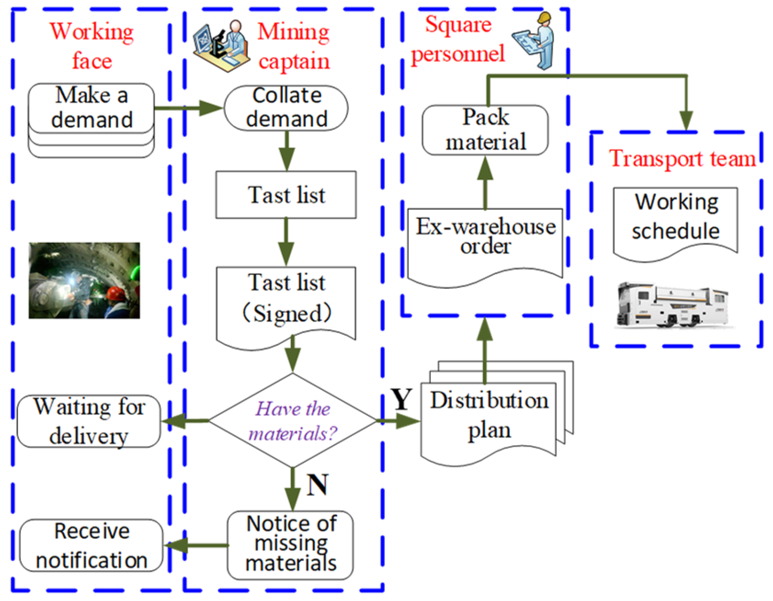
The material delivery process is shown in Figure 1. Working face to fill in the required material information submitted to take the mining captain for approval. Approval by the demand can be directly collated, approval does not pass the need to fill out the reasons for rejection. The working face checked the reasons for rejection and modified the material application form. After the modification was completed, the material application form was submitted to the mining captain for approval. Take the mining captain to audit all requirements after the formation of the task list and signed. The mining captain confirms whether the materials of the industrial square meet the requirements of the task list. When the materials in the industrial square meet the requirements of the task list, the distribution plan is formulated, and the working face waits for the delivery. The square personnel loads the materials into the standard container according to the Ex-warehouse order. After the loading is completed, the transport team transports according to the working schedule. When the material in the industrial square does not meet the requirements of the task list, the mining captain sends a material shortage notice to the working face, and the working face accepts the material shortage notice and modifies the application.

The material loading takes the intelligent loading vehicle of the industrial square as the starting point. The equipment layout of the industrial square is shown in Figure 2. In order to facilitate the loading and unloading of materials and standard containers, the transportation track is designed as a double track, with platform vehicles consisting of two platform vehicles. First of all, the square personnel puts the materials to be delivered according to the task list in advance, then the intelligent loading vehicle puts the materials into the empty standard container, and finally, the intelligent loading vehicle grabs the full standard container and fixes it on the empty platform vehicles after loading is completed by the transport robot in accordance with the planned route distribution. When the robot carries the empty standard container platform vehicles back, the intelligent loading vehicle grabs the empty standard container and puts it in the specified position.

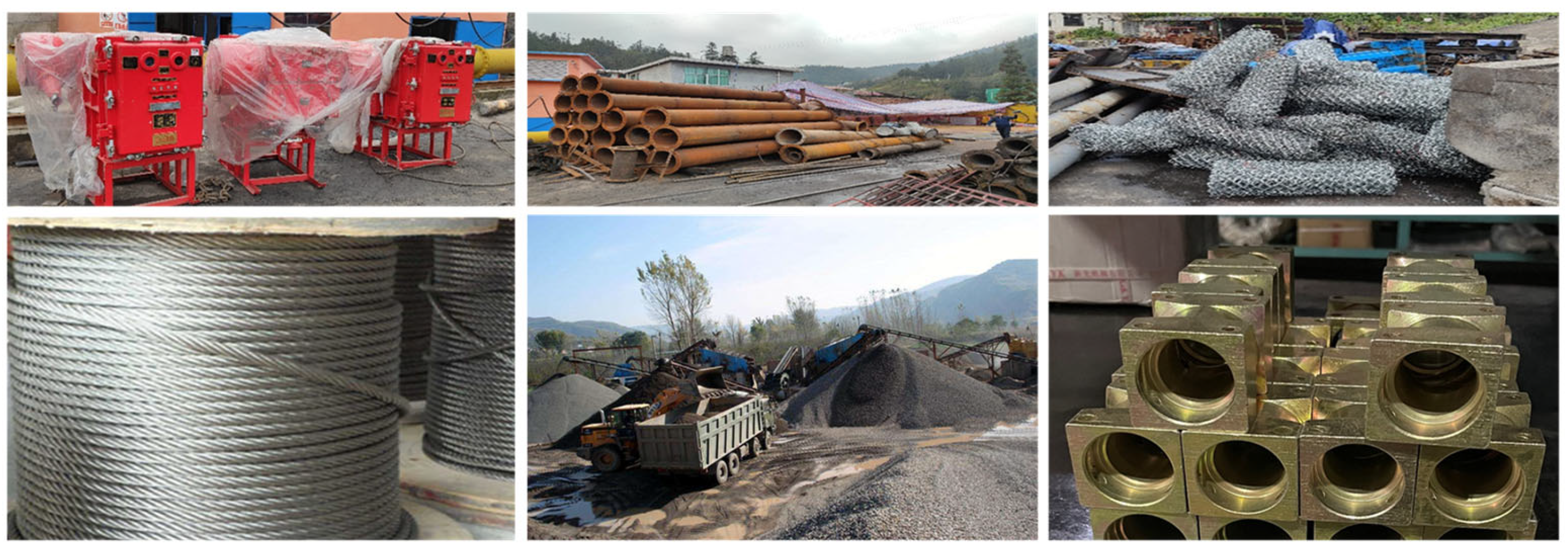
For the coal mine auxiliary transportation system, the types of distribution materials are complicated, as shown in Figure 3. These types of distribution materials include mechanical and electrical products (including wire and cable, high and low voltage electrical appliances, instruments and meters, lighting appliances, electronic components, etc.), metal materials (including ferrous metal materials, metal processing parts, non-ferrous metal materials, etc.), non-metallic materials (including wood, sand, asbestos products, refractory materials, glass, bricks and tiles, rubber and plastic products, etc.), labor protection products (including labor protection protective clothing, head protective equipment, labor toolkit, respiratory protective equipment, hand protective equipment, etc.), chemical products (including ultra-high molecular weight polyethylene, polyvinyl chloride pipe, polyethylene pipe, grease, coolant, etc.), coal washing accessories (including screening machinery, sorting machinery, dehydration machinery, etc.), fully mechanized mining accessories (including shearer, hydraulic support, winch, etc.), and fully mechanized mining equipment (including coal mining machine, coal mining machine, etc.). These materials (some up to a few meters and some only a few centimeters) have size differences. Some are solid, some are liquid, and some have different forms. Measuring units have weight units, length units, and quantity units, which are difficult to unify. In different types of work, the district team received materials may vary, the district team received a large number of personnel materials.

3. Establishment of Coal Mine Material Multi-Objective Scheduling Mathematical Model

3.1. Symbol Definition

The working face puts forward the material application according to the production demand, and forms i task list. The task list contains the basic characteristics of the material, and the material is loaded into the standard container according to the material characteristics. A three-dimensional rectangular coordinate system is established with the left, back, and bottom vertices of the standard container as the origin. The position decision variables ${\mathrm{x}}_{ick},{\mathrm{y}}_{ick}{,\mathrm{z}}_{ick}$ represent the coordinate values of the left, rear, and lower vertices of the material c in the standard container k in the X, Y, and Z directions, respectively. 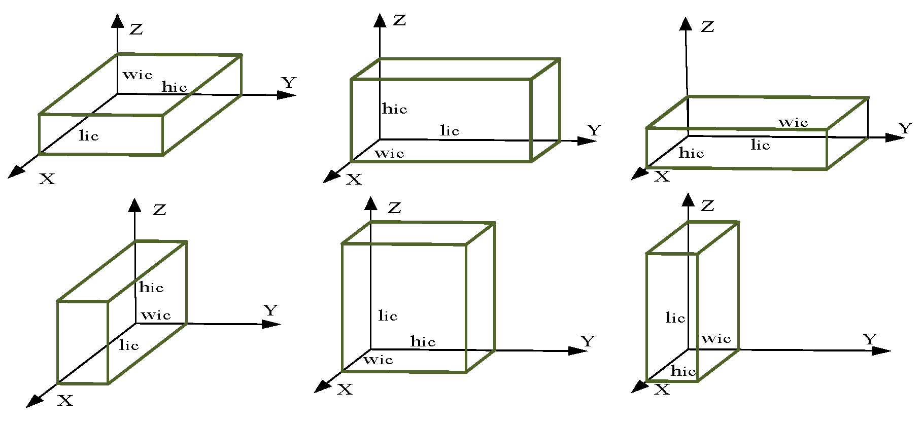Let ($\stackrel{-}{{\mathrm{x}}_{ick}},\stackrel{-}{{\mathrm{y}}_{ick}},\stackrel{-}{{\mathrm{z}}_{ick}}$) be the coordinates of another vertex of the body diagonal connected to the vertex, then the values can be calculated by the position decision variable and the relative length, width, and height, respectively. The materials are arranged in standard containers according to their length, width, and height {${\mathrm{l}}_{ic},{\mathrm{w}}_{ic}{,\mathrm{h}}_{ic}$}. There are six orthogonal placements, represented by the direction number ${\mathrm{p}}_{ic}$, as shown in Figure 4. The side of the material box parallel to the X-axis is relatively long, represented by $l_{ic}^X$; correspondingly, the material box is parallel to the edges of the Y and Z axes, which are relatively wide $h_{ic}^Y$ and relatively high $w_{ic}^Z$, respectively, as shown in

Table 1. Number of directions of material placement.

pic	${\mathit{l}}_{\mathit{i}\mathit{c}}^{\mathit{X}}$	${\mathit{h}}_{\mathit{i}\mathit{c}}^{\mathit{Y}}$	${\mathit{w}}_{\mathit{i}\mathit{c}}^{\mathit{Z}}$
1	lic	hic	wic
2	lic	wic	hic
3	wic	lic	hic
4	wic	hic	lic
5	hic	lic	wic
6	hic	wic	lic

.

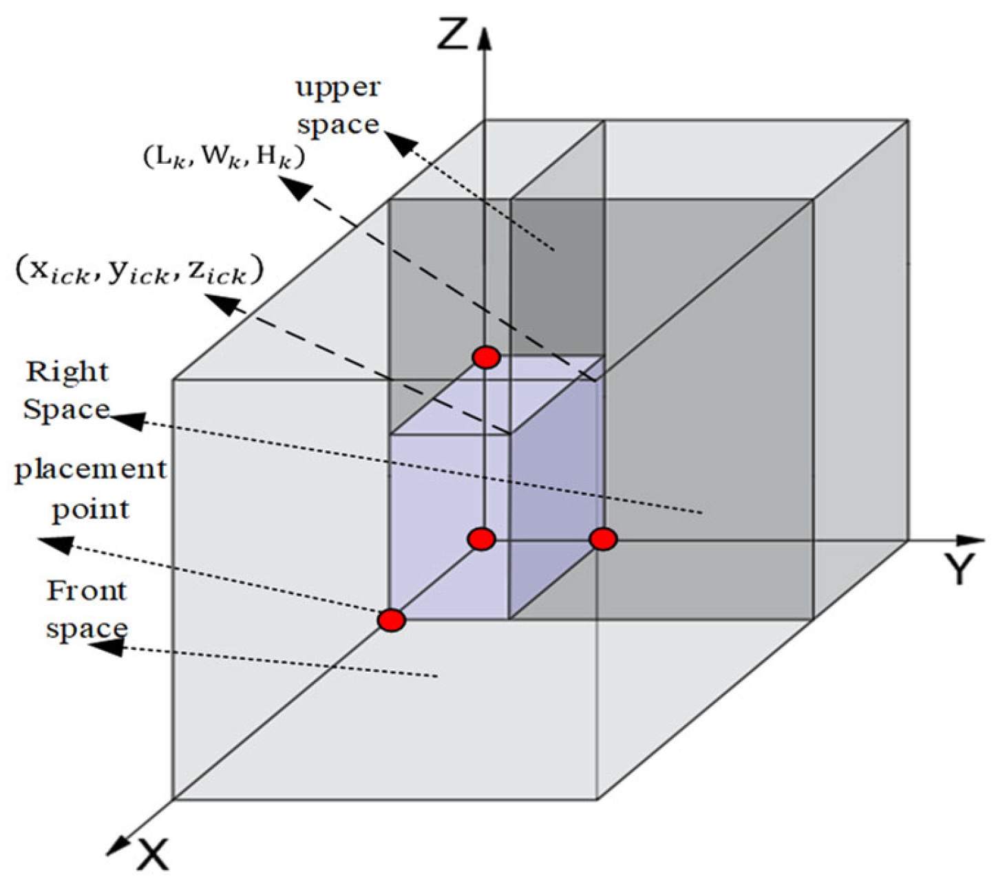
After the materials are loaded, the delivery process is described as a graph $\mathrm{G}(\mathrm{O},\mathrm{E})$, where $\mathrm{O}=\left\{o_i|i=\mathrm{0,1},2,\cdots ,n\right\}$ is the set of industrial squares and n working faces, $\mathrm{E}=\{v_i\to v_j|i,j=\mathrm{0,1},2,\cdots ,n\cap i\ne j\}$ is the set of all edges between the working faces. The distance between vertices $o_i,o_j$ is represented by $d_{ij}$. The robot carries a standard container from the industrial square to distribute materials to all working faces and returns to the industrial square after distribution. In the process of distribution, in order to improve the utilization rate of distribution resources and help the green development of coal mine transportation, it is necessary to minimize the use of robots and optimize the distribution path reasonably. The model involves mathematical parameter definitions as shown in

Table 2. Parameter definition of mathematical model.

Parameter	Meaning
$N=\{\mathrm{0,1},2,\dots n\}$	Working face and industrial square set, 0 for industrial square
${\mathrm{N}}^{\prime }=\{\mathrm{1,2},\dots \mathrm{n}\}$	Working face set
$\mathrm{E}=\left\{\right(i,j\left)\right|iϵN,jϵN,i\ne j\}$	Robots run from i to j
${\mathrm{d}}_{ij}=(iϵN,jϵN)$	Distance from i to j
${\mathrm{t}}_{ij}=(iϵN,jϵN)$	Time it takes for a robot to run from i to j
${\mathrm{s}}_i\left(iϵN\right)$	Requested arrival time for i
$M=\{\mathrm{0,1},2,\dots m\}$	Robot set, where m is the number of robots used
${\mathrm{G}}_m\left(mϵM\right)$	Rated load weight of robot
${\mathrm{t}}_{mi}=(mϵM,iϵN)$	Time robot m reaches i
$K=\{\mathrm{0,1},2,\dots k\}$	Standard container set, where k is the number of standard containers used
${\mathrm{L}}_k,{\mathrm{W}}_k{,\mathrm{H}}_k\left(kϵK\right)$	Length, width, and height of standard container k
${\mathrm{G}}_k\left(kϵK\right)$	Maximum load weight of standard container
${\mathrm{V}}_k\left(kϵK\right)$	Volume of standard container
${\mathrm{C}}_i=\{\mathrm{1,2},\dots \mathrm{C}|iϵ{\mathrm{N}}^{\prime }\}$	Working face i demand material collection, C is the amount of material required for i
${\mathrm{l}}_{ic},{\mathrm{w}}_{ic}{,\mathrm{h}}_{ic}(iϵ{\mathrm{N}}^{\prime },\mathrm{c}ϵ{\mathrm{C}}_i)$	Length, width, and height of medium material c in working face i
${\mathrm{X}}_k,{\mathrm{Y}}_k{,\mathrm{Z}}_k\left(\mathrm{k}ϵK\right)$	${\mathrm{L}}_k,{\mathrm{W}}_k{,\mathrm{H}}_k$ direction coordinates of the standard container
${\mathrm{x}}_{ick},{\mathrm{y}}_{ick}{,\mathrm{z}}_{ick}(iϵ{\mathrm{N}}^{\prime },\mathrm{c}ϵ{\mathrm{C}}_i,\mathrm{k}ϵK)$	The material c of the working face i is placed after the standard container k, and the coordinate of the lower left corner of the material is
$\stackrel{-}{{\mathrm{x}}_{ick}},\stackrel{-}{{\mathrm{y}}_{ick}},\stackrel{-}{{\mathrm{z}}_{ick}}(iϵ{\mathrm{N}}^{\prime },\mathrm{c}ϵ{\mathrm{C}}_i)$	The material c of the working face i is placed after the standard container k, and the coordinate of the upper right corner of the material is
${\mathrm{p}}_{ic}(iϵ{\mathrm{N}}^{\prime },\mathrm{c}ϵ{\mathrm{C}}_i)$	The placement direction of the material c of working face i, ${\mathrm{p}}_{iu}ϵ\left[\mathrm{1,6}\right]$
${\mathrm{g}}_{ic}(iϵ{\mathrm{N}}^{\prime },\mathrm{c}ϵ{\mathrm{C}}_i)$	The weight of the material c of the working face i

.

3.2. Model Construction

For ease of calculation, the following assumptions are made:

• All materials are packed in a cuboid box, called a material box.
• Single material does not exceed the standard container-rated load and volume.
• The material box must be placed inside the standard container (that is, in the three-dimensional coordinate system established in this paper, the coordinates of the upper right front corner of the material box cannot exceed the three-dimensional properties of the standard container).
• The two material boxes in the standard container cannot be spatially overlapped.
• The material box placed in the standard container needs to be placed parallel to the standard container, which is reflected in the three-dimensional coordinate system.
• Weight constraint: the total required weight of all working faces on one path cannot exceed the rated vehicle loading weight G_m.
• Direction constraint: some types of material boxes placed in the standard container direction cannot be arbitrarily rotated, only by some fixed edge as a high attribute.
• Support constraints: All bins placed need to have a support area. All the bottom areas of the bins need to be other bins or need to have a standard container bottom support.
• All the materials required for the working face are in the industrial square; that is, all the robots are hoisted from the industrial square.
• All robot types are consistent.
• Each working face can only be distributed by one robot; that is, the demand is inseparable.
• The number of robots is related to the number of paths. A robot distributes a working face on a path, and it cannot be sent or leaked.
• The ‘first in and then out’ constraint. In the same path, the materials that serve the working face first need to be unloaded first, and the unloading process cannot be hindered by the materials of other working faces.
• Priority sorting. The working face requires urgent priority delivery.

Three two-valued variables ${\alpha }_{ck}\in \left\{\mathrm{0,1}\right\}$, ${\beta }_{km}\in \left\{\mathrm{0,1}\right\}$, ${\gamma }_{ijm}\in \left\{\mathrm{0,1}\right\}$ are defined. If the material c is completed by the standard container k, then ${\alpha }_{ck}=1$, otherwise, ${\alpha }_{ck}=0$; if the material of the standard container k is completed by the robot m, then ${\beta }_{km}=1$, otherwise, ${\beta }_{km}=0$; if the robot m runs from i to j, then ${\gamma }_{ijm}=1$, otherwise, ${\gamma }_{ijm}=0$.

In this paper, the robot path optimization model with the highest three-dimensional loading rate of standard containers is established with the minimum number of delivery vehicles and the shortest delivery path as the research objectives.

Objective function:

$$\mathrm{m}\mathrm{i}\mathrm{n}{Z}_1=\sum _{i=0}^N\sum _{c=0}^{{\mathrm{C}}_i}K$$

(1)

$$\mathrm{m}\mathrm{i}\mathrm{n}{Z}_2=\sum _{i=0}^N\sum _{j=0}^N\sum _{m=0}^M{d}_{ij}{\gamma }_{ijm}$$

(2)

$$\mathrm{m}\mathrm{i}\mathrm{n}{Z}_3=\sum _{j=0}^N\sum _{m=0}^M{\gamma }_{0jm}$$

(3)

$$\mathrm{m}\mathrm{i}\mathrm{n}{Z}_4=\sum _{i=0}^N\sum _{m=0}^M{\mathrm{t}}_{mi}-{\mathrm{s}}_i$$

(4)

In Formula (1), K denotes the number of standard containers. In Formula (2), $\sum _{i=0}^N\sum _{j=0}^N\sum _{m=0}^M{d}_{ij}{\gamma }_{ijm}$ denotes the total distance from all materials to the working face. In Formula (3), $\sum _{j=0}^N\sum _{m=0}^M{\gamma }_{0jm}$ denotes the total number of robots starting from the industrial square. In Formula (4), ${\mathrm{t}}_{mi}-{\mathrm{s}}_i$ denotes the delayed delivery time of the robot.

Constraint conditions:

$$\sum _{c=0}^C{\mathrm{l}}_{ic}<{\mathrm{L}}_k,\sum _{c=0}^C{\mathrm{w}}_{ic}<{\mathrm{W}}_k,\sum _{c=0}^C{h}_{ic}<H_k\forall i\in N,\forall \mathrm{c}ϵ{\mathrm{C}}_i,\forall k\in K$$

(5)

$$\sum _{c=0}^C{g}_{ic}{\alpha }_{ck}\le {\mathrm{G}}_k\forall i\in N,\forall k\in K$$

(6)

$$\sum _{c=0}^C{\mathrm{l}}_{ic}{\mathrm{w}}_{ic}{\mathrm{h}}_{ic}{\alpha }_{ck}\le {\mathrm{V}}_k\forall i\in N,\forall k\in K$$

(7)

$$\begin{array}{c}{l}_{ic}^X=\left\{\begin{array}{c}{\mathrm{l}}_{ic}{\mathrm{p}}_{ic}=\mathrm{1,2}\\ {\mathrm{w}}_{ic}{\mathrm{p}}_{ic}=\mathrm{3,4}\\ {\mathrm{h}}_{ic}{\mathrm{p}}_{ic}=\mathrm{5,6}\end{array}\right.\forall i\in N,\forall \mathrm{c}ϵ{\mathrm{C}}_i\\ l_{ic}^Y=\left\{\begin{array}{c}{\mathrm{l}}_{ic}{\mathrm{p}}_{ic}=\mathrm{3,5}\\ {\mathrm{w}}_{ic}{\mathrm{p}}_{ic}=\mathrm{1,4}\\ {\mathrm{h}}_{ic}{\mathrm{p}}_{ic}=\mathrm{2,6}\end{array}\right.\forall i\in N,\forall \mathrm{c}ϵ{\mathrm{C}}_i\\ l_{ic}^Z=\left\{\begin{array}{c}{\mathrm{l}}_{ic}{\mathrm{p}}_{ic}=\mathrm{4,6}\\ {\mathrm{w}}_{ic}{\mathrm{p}}_{ic}=\mathrm{2,3}\\ {\mathrm{h}}_{ic}{\mathrm{p}}_{ic}=\mathrm{1,5}\end{array}\right.\forall i\in N,\forall \mathrm{c}ϵ{\mathrm{C}}_i\end{array}$$

(8)

$$\begin{array}{c}\stackrel{-}{{\mathrm{x}}_{ick}}={\mathrm{x}}_{ick}+l_{ic}^X\forall i\in N,\forall \mathrm{c}ϵ{\mathrm{C}}_i\\ \stackrel{-}{{\mathrm{y}}_{ick}}={\mathrm{y}}_{ick}+l_{ic}^Y\forall i\in N,\forall \mathrm{c}ϵ{\mathrm{C}}_i\\ \stackrel{-}{{\mathrm{z}}_{ick}}={\mathrm{z}}_{ick}+l_{ic}^Z\forall i\in N,\forall \mathrm{c}ϵ{\mathrm{C}}_i\end{array}$$

(9)

$$\max \left\{\frac{\max \left({\mathrm{x}}_{ick},{\mathrm{x}}_{idk}\right)}{\min \left(\stackrel{-}{{\mathrm{x}}_{ick}},\stackrel{-}{{\mathrm{x}}_{idk}}\right)},\frac{\max \left({\mathrm{y}}_{ick},{\mathrm{y}}_{idk}\right)}{\min \left(\stackrel{-}{{\mathrm{y}}_{ick}},\stackrel{-}{{\mathrm{y}}_{idk}}\right)},\frac{\max \left({\mathrm{z}}_{ick},{\mathrm{z}}_{idk}\right)}{\min \left(\stackrel{-}{{\mathrm{z}}_{ick}},\stackrel{-}{{\mathrm{z}}_{idk}}\right)}\right\}\ge 1\forall i\in N,\forall \mathrm{c},\mathrm{d}ϵ{\mathrm{C}}_i,\forall k\in K$$

(10)

when ${\alpha }_{ik}=1$ and ${\mathrm{z}}_{ick}>0$, ${\mathrm{x}}_{ick}\le x\le \stackrel{-}{{\mathrm{x}}_{ick}},{\mathrm{y}}_{ick}\le y\le \stackrel{-}{{\mathrm{y}}_{ick}}$ for $\forall i\in N,\forall \mathrm{c}ϵ{\mathrm{C}}_i,\forall x,y,z$, there exists $\mathrm{d}ϵ{\mathrm{C}}_i$ such that the following conditions are satisfied:

$$\begin{array}{c}{\mathrm{x}}_{idk}\le x\le \stackrel{-}{{\mathrm{x}}_{idk}}\\ {\mathrm{y}}_{idk}\le y\le \stackrel{-}{{\mathrm{y}}_{idk}}\\ {\mathrm{z}}_{ick}=\stackrel{-}{{\mathrm{z}}_{idk}}\end{array}$$

(11)

$${\mathrm{d}}_{ij}=t_{ij}\forall i,j\in N$$

(12)

$${\mathrm{t}}_{m0}=s_0=0 \forall m\in M$$

(13)

$$\sum _{j=0}^N\sum _{m=0}^M{\gamma }_{ijm}=1,\forall i\in N$$

(14)

$${\sum }_{k=0}^K{\mathrm{G}}_k{\beta }_{km}\le {\mathrm{G}}_m,\forall m\in M$$

(15)

$$\sum _{m=0}^M{\gamma }_{0jm}=1,\forall m\in M$$

(16)

$$\sum _{i=0}^N{\gamma }_{izm}-\sum _{j=0}^N{\gamma }_{zjm}=0 \forall z\in N,\forall m\in M$$

(17)

$$\sum _{i=0}^N{\gamma }_{iom}=1,\forall m\in M$$

(18)

The Formula (5) represents the length-width-height constraint; that is, the three-dimensional size of the container for a single material is smaller than that of the standard container. The Formula (6) represents the load constraint, the container weight of a single material is less than the maximum load-bearing weight of the standard container. Equation (7) represents the volume constraint, the container volume of a single material is less than the standard container volume. The Formula (8) represents the value of the relative length, width, and height of the material container in different directions. Equation (9) represents the calculation method of the upper right corner of the material container and also suggests that the container must be placed parallel to the standard container. The Formula (10) denotes the non-overlapping constraints of c and d in the container space. Equation (11) represents the support constraint, c material container must have a standard container bottom or material container d support. Equation (12) indicates that the robot’s running speed is 1 m/s; that is, the spatiotemporal conversion coefficient is 1, and the space and time values are equal. Equation (13) represents the data initialization of the industrial square. The time at which the robot first reaches the industrial square and the working time in the industrial square are both 0. Equation (14) indicates that each working face is accessed and only accessed once. Equation (15) means that the weight of the standard container carried by the robot does not exceed its rated load. Equations (16)–(18) indicate that all robots start from the industrial square and return to the industrial square after several non-repetitive working faces.

4. Coal Mine Material Multi-Objective Scheduling Mathematical Model Solution

4.1. Coal Mine Material Multi-Objective Scheduling Mathematical Model Solution

Three-dimensional loading is a typical NP-hard problem, and the heuristic algorithm has a good solution to this kind of problem. The realization of the whole loading process is to show the placement order and placement position of the material box, and the influence on the spatial layout of the standard container. In this paper, the heuristic algorithm of three-dimensional space segmentation is used to solve the loading scheme. For the heterogeneity of materials, the corresponding loading strategy is formulated as follows.

4.1.1. Determine the Loading Sequence

Material box size and different loading sequences produce different standard container space layouts, at the beginning of loading, need to determine the material box loading sequences, and generally adopt the method of decreasing volume, length, weight, etc. Taking the volume decreasing rule of the material box as an example, the volume of the material box is sorted. If the volume is equal, the length, width, and high attributes are considered in turn. If the length, width, and high attributes of the material are the same, the weight of the material is considered. For the same specifications of the material, the placement order can be regardless of the order.

4.1.2. Determine the Material Placement Position

After the material loading sequence is clarified, rules need to be formulated to determine its relative placement position. To make the remaining space of the standard container larger and more regular, the first material is placed in a corner of the standard container, and then loaded one by one along the edge.

4.1.3. Three-Dimensional Space Segmentation Method

After placing a material container c of size $({\mathrm{x}}_{ick},{\mathrm{y}}_{ick}{,\mathrm{z}}_{ick})$ into a standard container k of size $(L_k,W_k{,H}_k)$, the available space of the standard container has three parts, front, right and top, as shown in Figure 5. The space coordinate of the kth standard container is set as $\mathrm{R}=(\mathrm{k},\mathrm{0,0},0,L_k,W_k{,H}_k)$, where (0,0,0) is the coordinate of the placement point, and ${(L}_k,W_k{,H}_k)$ is the space length, width, and height coordinates. After being placed in the container c, the three newly generated space coordinates are as follows:

$$\left\{\begin{array}{c}{R}_1=\left(k,x_{ick},\mathrm{0,0},L_k,W_k{,H}_k\right)\\ R_2=\left(k,,0,y_{ick},0,x_{ick},W_k{,H}_k\right)\\ R_3=\left(k,\mathrm{0,0},{,z}_{ick},x_{ick},y_{ick}{,H}_k\right)\end{array}\right.$$

(19)

4.1.4. Space Merge Method

When a standard container is placed in a material box, three free spaces are generated. When a free space is selected to be placed in the second material box, three free spaces are generated again in the free space. With the addition of the material box one by one, the free space presents many small characteristics. These free spaces are too small to accommodate the material box, which reduces the space utilization of the standard container. In order to increase the utilization rate of free space, the free space is merged in the following ways: First, the left and right are merged. When the two adjacent free spaces X and Z are the same, they can be merged into a larger free space. The second is to merge before and after. When the two adjacent free spaces have the same Y and Z coordinates, they can be merged into a larger free space. The third is to merge up and down. When two adjacent free space X and Y coordinates are the same, they can be merged into a larger free space.

4.1.5. Same Material Box Merging Rules

According to the rules of space division and merger, it is found that the generation of small free space is related to the number of material boxes. The more material boxes, the more the small free space. In order to reduce the number of small free spaces, the number of material boxes can be reduced, that is, the combination of the same specifications and models in the task list to piece together a larger ‘material box’. The combination of material boxes refers to the combination of the same material boxes according to the same placement posture. The material boxes have six placement postures, and the placement posture is selected with the maximum space utilization rate as the goal. The three-dimensional size of the combined large ‘material box’ is smaller than the three-dimensional size of the standard container, and the weight does not exceed the maximum weight limit of the standard container.

The specific steps of the three-dimensional space heuristic algorithm are shown in Figure 6:

• Input standard container size and quantity, material box three-dimensional size, and weight.
• Call the material box merging algorithm to merge the same specification material boxes into new material boxes and arrange the material boxes according to the loading sequence.
• Initialize the standard container space, search the free space, determine whether the material box can be placed in the free space, and assess whether the material box can be placed; if the material box cannot be placed, traverse the remaining material box. If all the material boxes cannot be placed, select the next standard container.
• Determine the location of the material box and divide the three-dimensional space of the standard container.
• Call space merging algorithm to generate new free space and delete the corresponding free space before merging.
• Repeat the above steps until the goods are loaded.

4.2. Dual-Layer Genetic Algorithm to Optimize Multi-Objective

The dimensional loading constraints (3L-VRPTW) studied in this paper are a typical multi-objective optimization problem. When solving multi-objective decision making, there are two main methods, one is the composite type, multi-objective decision making into single-objective decision making; the other is hierarchical. In the case of ensuring the first goal, trying to optimize the second and third goals is necessary. In order to solve the non-inferior solution of the multi-objective programming problem, the multi-objective programming problem is often transformed into a single-objective programming problem. The methods to achieve the transformation are as follows: the evaluation function method, goal programming method, hierarchical sequence method, and intelligent optimization algorithm, such as NSGA-II. In this paper, the number of optimization standard containers in the four optimization objectives is relatively independent compared to the optimization of distribution path parameters. The solution process has been introduced previously. The remaining three optimization objectives are related to the number of distribution times. The more the number of distribution times, the longer the total distribution distance, and the more the number of robots needed, but the delay distribution time will be reduced. Each working face is distributed separately, with the shortest delay time and the highest cost. In order to balance the three optimization objectives, firstly, the standard genetic algorithm is used to solve the shortest distance, then the NSGA-II algorithm structure is used to solve the Pareto optimal solution set of the number of robots and the delay time, and finally, the optimal distribution parameters are output through the elite selection mechanism.

4.2.1. Coding Method

The coding method is integer coding. Assume that the industrial square has four working faces for material delivery, and the initial delivery path code can be [0, 1, 3, 0, 2, 4, 0], as shown in Figure 7. Among them, 0 represents the industrial square, and other numbers represent each working face. According to the constraints of the standard container grouping of the auxiliary transportation robot and the maximum load capacity of the robot, the chromosome is decoded with the natural number 0 to form the corresponding sub-path. It can be seen from Figure 7 that the chromosome can be decoded into two sub-paths of [0, 1, 3, 0] and [0, 2, 4, 0]; that is, the distribution path of robot M1 is as follows: industrial square 0 → working face 1 → working face 3 → industrial square 0. The distribution path of robot M2 is as follows: industrial square 0 → working face 2 → working face 4 → industrial square 0.

4.2.2. Crossover Operation

The cross-operation mode is 2-opt*, that is, the random algorithm, as shown in Figure 8. The specific implementation method involves assuming the working surface $i ϵ {\mathrm{N}}^{\prime },j ϵ {\mathrm{N}}^{\prime }$, and the distribution route ${\mathrm{R}}_i=[0,\dots ,\mathrm{i}+1,\mathrm{i}+2,\dots ,0]$, the distribution route ${\mathrm{R}}_j=[0,\dots ,\mathrm{j}+1,\mathrm{j}+2,\dots ,0]$. Using 2-opt * crossover to generate a new delivery route $R_i^{\prime }=[0,\dots ,\mathrm{j}+1,\mathrm{j}+2,\dots ,0]$, $R_j^{\prime }=[0,\dots ,\mathrm{i}+1,\mathrm{i}+2,\dots ,0]$. After the crossover operation, the distribution scheme corresponding to the robot path should meet the relevant constraints. If not, the crossover operation should be re-performed. The objective function value and crowding degree of individuals after the exchange are calculated and arranged in descending order. The parent population is generated by the elite strategy.

4.2.3. Variation Operation

In order to increase the global search ability of the algorithm, the mutation operation is adopted, as shown in Figure 9. The specific implementation method is as follows: according to the mutation probability value Pm, two genes in one chromosome of the parent generation are randomly selected for exchange to generate a new offspring chromosome. After the mutation operation, the distribution scheme corresponding to the robot path should meet the relevant constraints. If not, the mutation operation should be carried out again.

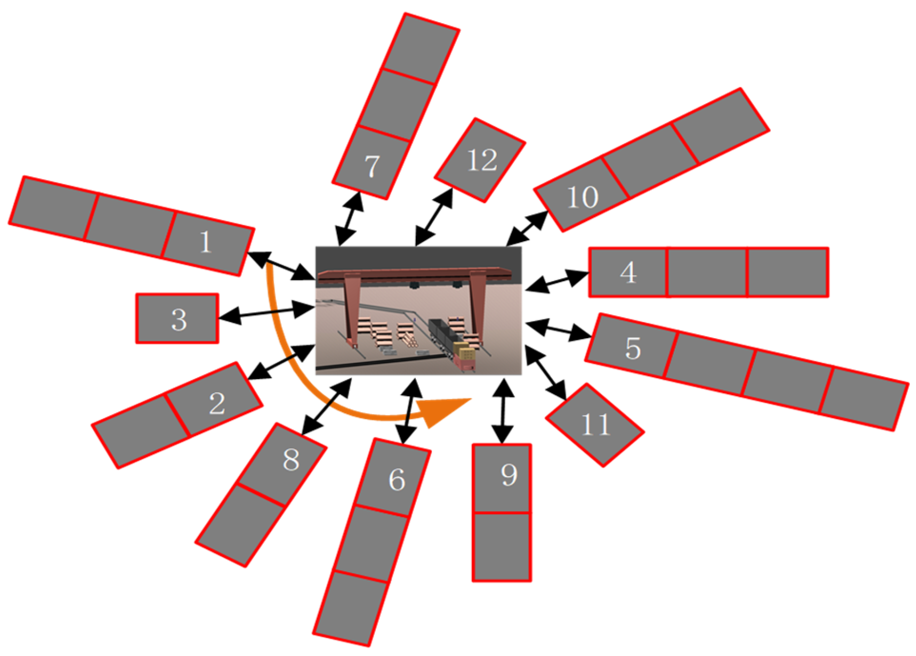
5. Application Analysis

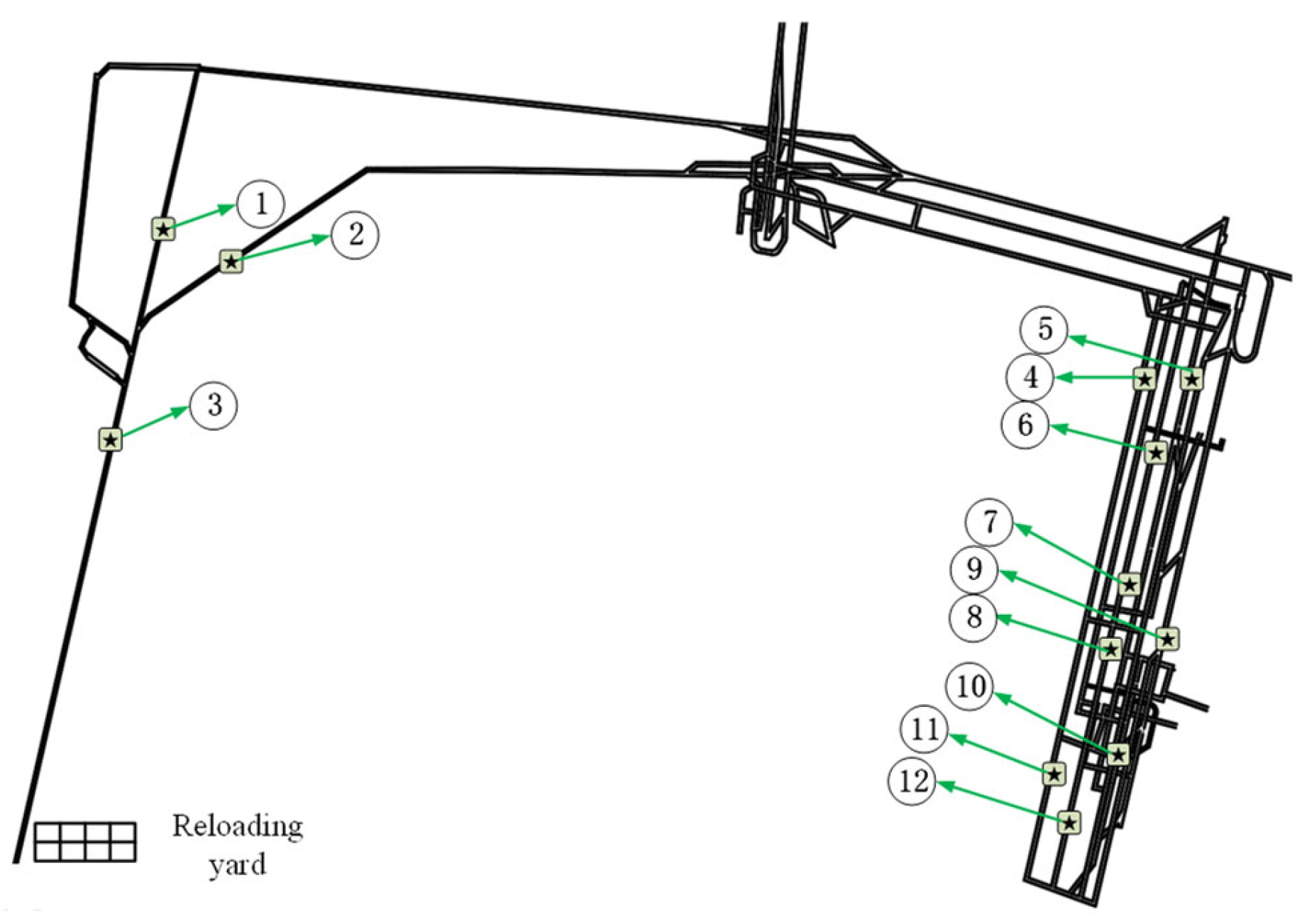
Twelve task orders in the third mining area were randomly selected for research, and the reloading yard was used as the origin to measure the task list destination coordinates. The specific working face distribution is shown in Figure 10.

Table 3. Parameters of working face.

Task List Code	1	2	3	4	5	6	7	8	9	10	11	12
Ideal time	8:32	8:44	8:36	15:00	14:54	10:25	16:50	9:20	10:30	16:00	14:00	16:15
horizontal scale	275	200	116	1532	1599	1550	1510	1488	1555	1490	1400	1450
vertical scale	819	870	490	648	677	572	388	304	325	148	130	60

shows the task list parameter information of a specific working face, including the task list code, the ideal delivery time of the material, and the coordinates of the working face. The ideal delivery time of the material is determined when the working face applies to the material. The materials and related information required in the task list are shown in

Table 4. Task list of material parameters.

Task List 1					Task List 2					Task List 3
code	length	width	height	weight	code	length	width	height	weight	code	length	width	height	weight
013	542	321	339	1669	019	941	938	91	257	031*50	449	100	314	45
007	2498	771	423	1528	025	1087	379	816	1076	037*70	400	123	169	27
012	915	979	62	178	016	615	662	242	315
009*2	2453	646	750	3803	030	1394	383	345	589
014	850	262	180	128	026	823	998	358	941
010	194	411	909	232	029	360	558	287	184
015	533	717	18	22	022	751	396	346	329
011	367	836	156	153	028*2	76	508	656	81
003	478	415	964	612	027	1825	758	607	2687
002	2371	612	329	1528	023	598	523	775	776
004	1794	202	995	1154	020	1204	624	866	2082
001	1429	852	425	1669	018	2835	585	67	356
005	2720	675	84	494	024	2197	864	4	24
006	1859	26	879	136	021	1859	26	879	136
008	1385	142	12	8
Task List 4					Task List 5					Task List 6
code	length	width	height	weight	code	length	width	height	weight	code	length	width	height	weight
070	1793	988	589	4598	045*2	2770	873	675	5223	078	73	729	101	17
065	461	39	115	065	049	55	828	407	59	079	1228	30	596	70
068*4	971	41	187	1754	050	1288	96	629	249	073	859	56	623	96
067	1026	916	994	385	048	597	91	200	35	076	2366	930	614	4323
066	2785	708	204	1287	047	760	711	215	372	075	2162	474	907	2974
064	525	254	902	385	042	587	518	804	782	077	1627	396	831	1713
061	2399	785	763	4598	046*3	938	849	947	2413	080	2751	708	110	686
063	1690	412	787	1754	051	2672	787	16	108	082	2128	614	648	2709
071	782	465	952	1108	041	2874	553	396	2014	072	2860	303	91	252
069	2578	940	311	2412	044	2271	101	562	413	081	1196	907	233	809
					043	2187	360	775	1953
Task List 7					Task List 8					Task List 9
code	length	width	height	weight	code	length	width	height	weight	code	length	width	height	weight
093	357	30	828	28	097	1748	290	53	86	046	938	849	947	2413
083	795	831	713	1507	102	649	643	728	972	108*8	490	538	785	662
088	1163	609	732	1659	099	359	561	884	570	065	461	39	115	7
092	1327	729	65	201	100	2956	436	757	3122	103	642	708	968	1408
090	2809	930	325	2717	094	266	44	234	495	106	913	822	112	269
085	1774	465	948	2502	095	420	808	602	570	105	1939	515	437	1396
084	2139	988	27	183	101	1486	64	57	3122	109	1658	951	360	1816
086	2248	303	206	449	096	2688	149	661	847	104	1685	225	259	314
089	1587	474	244	587	098	2451	106	595	495
091	2807	394	84	297
087	2153	56	348	134
Task List 10					Task List 11					Task List 12
code	length	width	height	weight	code	length	width	height	weight	code	length	width	height	weight
020*2	91	938	941	257	009	2453	750	646	3803	047*8	760	711	215	372
023*10	775	598	523	776	013*15	339	321	542	189	071*2	782	465	952	1108
030	1394	383	345	589	015*60	533	18	717	22	023*2	775	598	523	776
017*2	2330	472	153	538						011*2	367	836	156	153
										028*10	76	656	508	81

. The material coding column in Table 4 contains information about the number of materials and the number of omitted individual materials. The parameter unit of material length, width, and height is a millimeter, and the parameter unit of weight is the kilogram. It can be seen from the table that material types are quite different and heterogeneous. Now it is necessary to load the materials in the task list into standard containers with a length of 3 m, a width of 1 m, and a height of 1 m, and calculate the number of standard containers required.

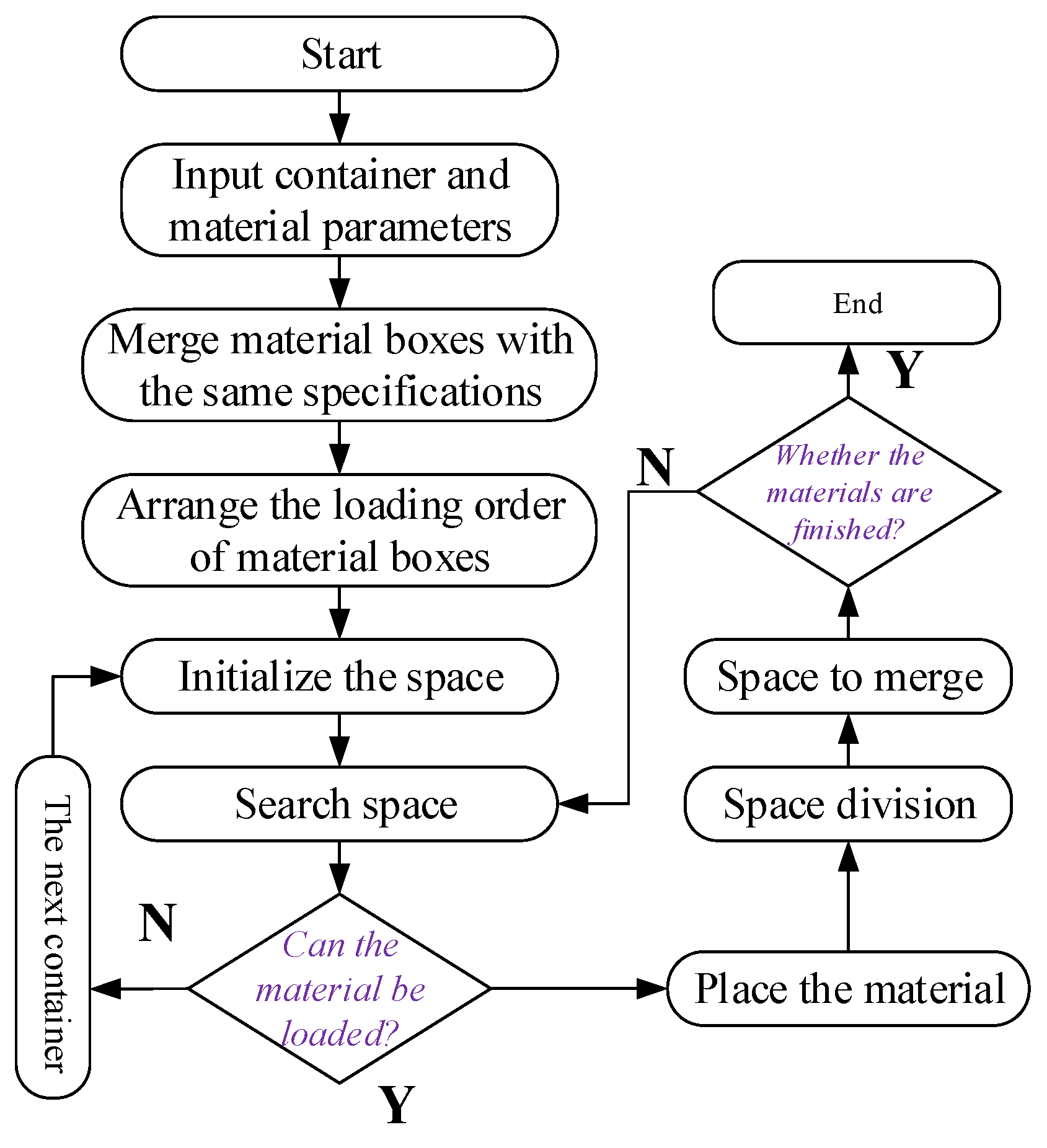
The three-dimensional space segmentation heuristic algorithm is used to solve the 12 task list loading schemes, and the number of standard containers required for each task list and the space utilization rate of each standard container in a single task list are calculated. The number of standard containers and the maximum space utilization rate of standard containers in a single task list are shown in

Table 5. Intelligent loading result.

Task List Code	1	2	3	4	5	6	7	8	9	10	11	12
Number of containers	3	2	1	3	4	3	3	2	2	3	1	1
loading rate	81%	71%	47%	77%	82%	63%	76%	60%	79%	65%	83%	82%

. It can be seen from the intelligent loading results in Table 5 that when there are few materials on the task list, only a standard container is needed, which can be called a single-container task list. The loading rate of a single-container task list container is the sum of the volume of all materials in the task list and the volume of the standard container. When there are many materials on the task list, two or more standard containers are needed to complete the material, which can be called a multi-container task list. The maximum space utilization rate of the standard container in the multi-container task list is smaller than that of the single-container task list. The difference is mainly caused by the strength of the material heterogeneity. The stronger the material heterogeneity, the lower the maximum space utilization rate of the standard container.

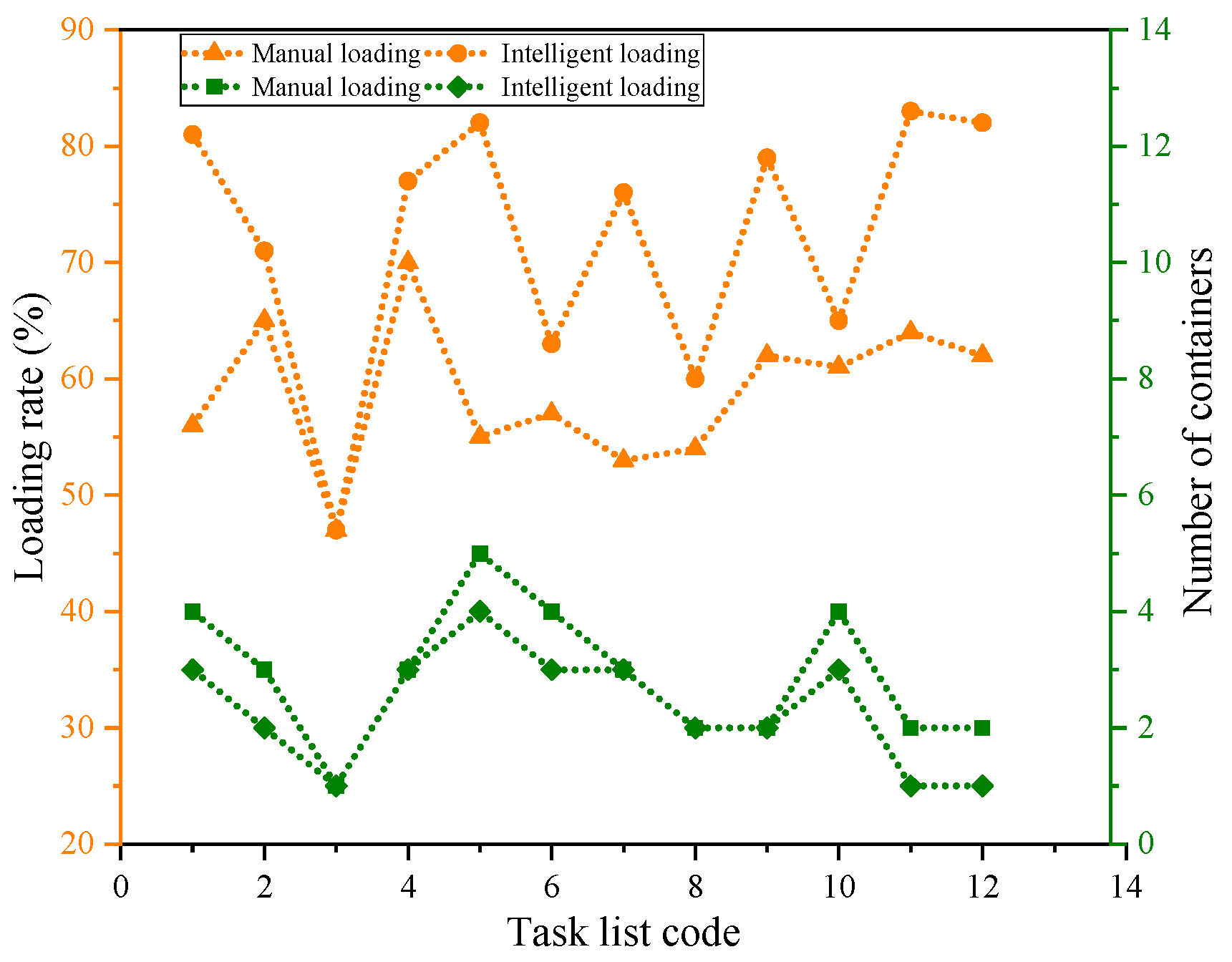
Statistical manual loading results are shown in

Table 6. Manual loading result.

Tast List Code	1	2	3	4	5	6	7	8	9	10	11	12
Number of containers	4	3	1	3	5	4	3	2	2	4	2	2
loading rate	56%	65%	47%	70%	55%	57%	53%	54%	62%	61%	64%	62%

. The performance diagrams of different loading modes are drawn according to the loading results, as shown in Figure 11. The manual loading results of a single-container task list are less, the multi-container task list standard container maximum space utilization difference is small, and, overall, they are full of subjectivity. Comparing the two loading methods, from the perspective of the maximum space utilization rate of the standard container, the average space utilization rate of the maximum space utilization rate of the manual loading standard container is 59%, the average space utilization rate of the maximum space utilization rate of the intelligent loading standard container is 72%, and the intelligent loading is 18% higher than the average space utilization rate of the manual loading. From the number of standard containers, 12 task lists are manually loaded using 35 standard containers, and 12 task lists are intelligently loaded using 28 standard containers. Intelligent loading reduces the use of standard containers by 20% compared with manual loading. In general, intelligent loading has better performance than manual loading.

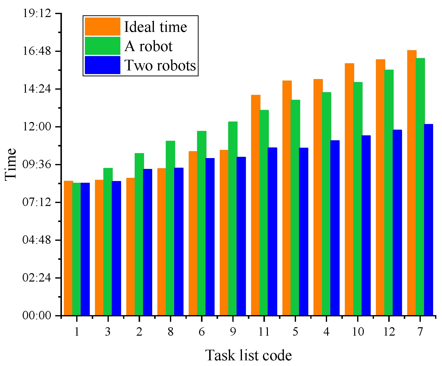
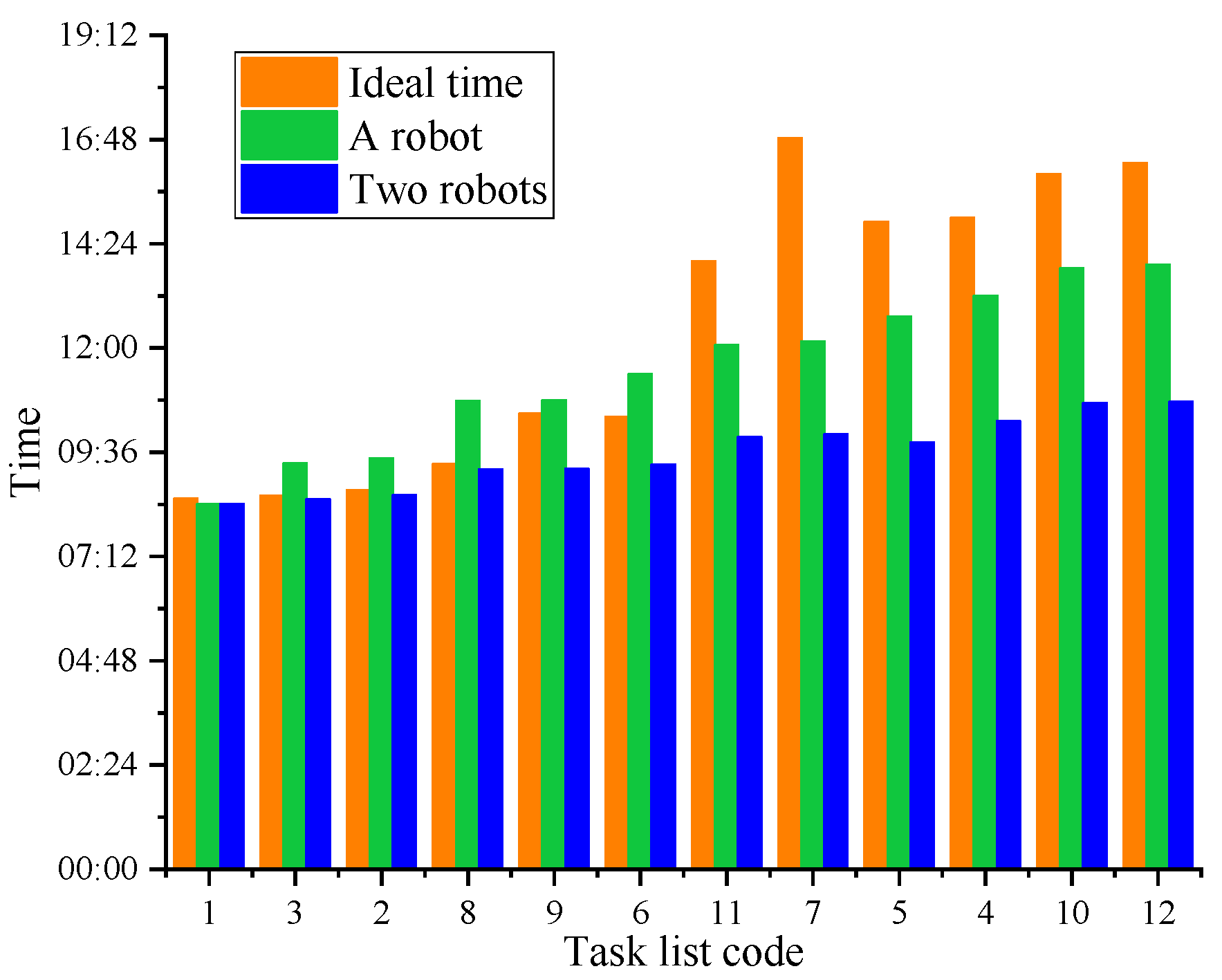
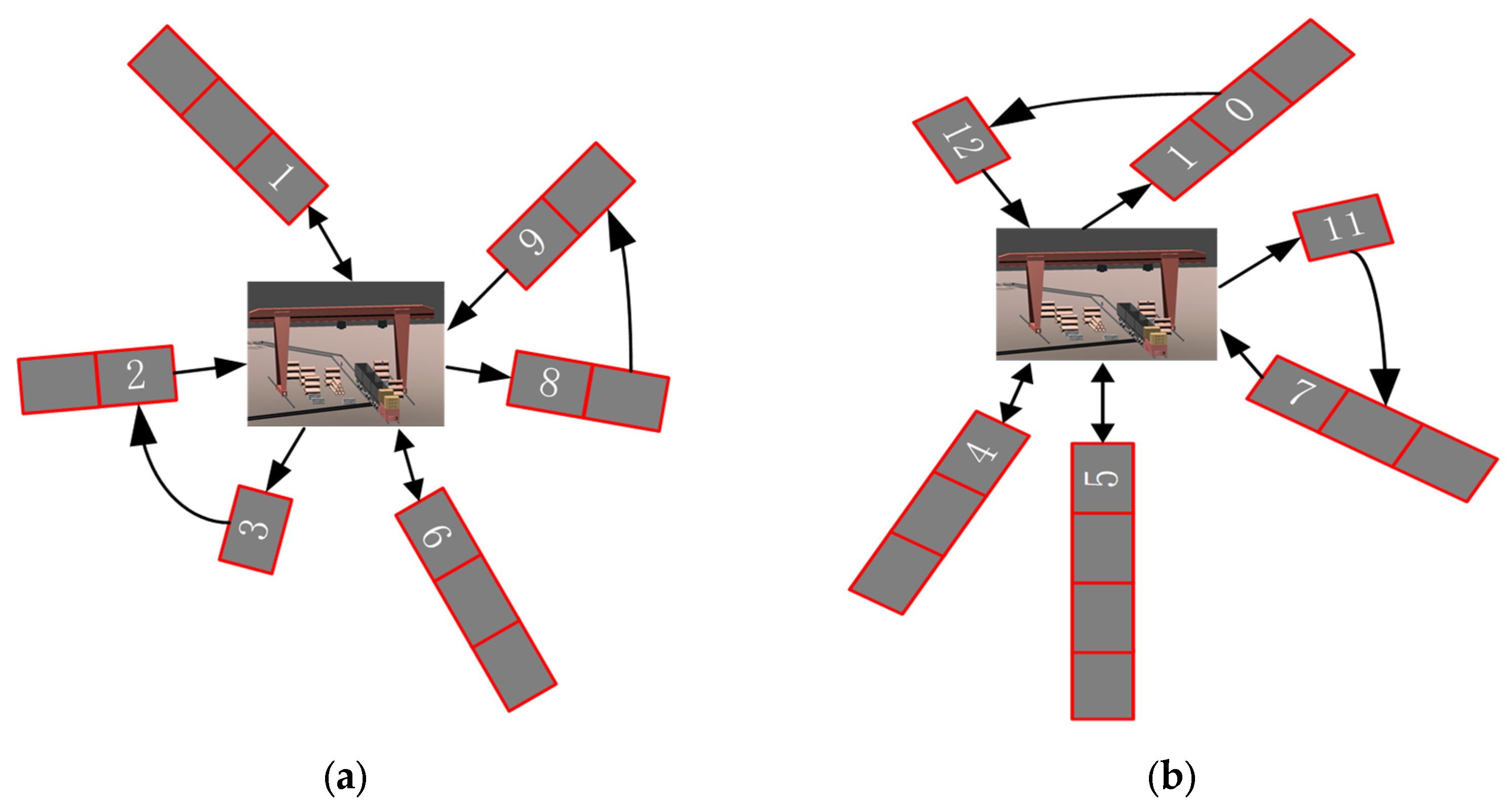
The electric locomotive robot is grouped into 4 groups with a maximum load of 20 t. The electric locomotive is manually scheduled to be loaded and dispatched according to the task list. If the task list material is within the carrying range of the electric locomotive, the task list is distributed by an electric locomotive. If the task list material is larger than the carrying range of the electric locomotive, the electric locomotive will carry out multiple distributions. The electric locomotive that distributes the task list does not accept the distribution of other task list materials. Under this delivery rule, the scheduling scheme is shown in

Table 7. Scheduling scheme.

Manual Scheduling		A Robot	Two Robots	Intelligent Scheduling		A Robot	Two Robots
Task list code	Ideal time	Actual time	Actual time	Task list code	Ideal time	Actual time	Actual time
1	8:32	8:25	8:25	1	8:32	8:25	8:25
3	8:36	9:21	8:31	3	8:36	9:21	8:31
2	8:44	10:18	9:17	2	8:44	9:28	8:37
8	9:20	11:05	9:22	8	9:20	10:47	9:12
6	10:25	11:42	9:59	9	10:30	10:48	9:13
9	10:30	12:18	10:03	6	10:25	11:24	9:19
11	14:00	13:02	10:39	11	14:00	12:04	9:57
5	14:54	13:41	10:38	7	16:50	12:09	10:01
4	15:00	14:10	11:07	5	14:54	12:43	9:50
10	16:00	14:48	11:25	4	15:00	13:12	10:19
12	16:15	15:36	11:47	10	16:00	13:50	10:44
7	16:50	16:20	12:08	12	16:15	13:55	10:46

, and the path planning is shown in Figure 12. The yellow arrows represent the delivery task list, which is in the task list of (0,1,0), (0,3,0), (0,2,0), (0,8,0), (0,8,0), (0,9,0), (0,11,0), (0,5,0), (0,4,0), (0,10,0), (0,12,0), (0,7,0). If there is only one electric locomotive robot on site, the total delivery distance under manual scheduling is 31,178.01 m, regardless of loading and unloading time. There are five delivery delay task lists (task list two, task list three, task list eight, task list six, and task list nine), as shown in Figure 13. The delay time is 15,772 s; if there are two electric locomotive robots available on site, regardless of the loading and unloading time, the number of delivery delay task lists is two (task list 2 and task list 8), and the delay time is 2088 s.

The experiment was carried out on a computer with a hardware configuration of AMD Ryzen 7 5800X 8-Core Processor 3.79 GHz, 32.0 GB, 3.79 GHz frequency, and the development environment was PyCharm2020.1 x64. The specific parameters are set as follows: population size pop size = 100, crossover probability Pc = 0.6, mutation probability Pm = 0.2.

The standard genetic algorithm optimizes the shortest delivery distance of 20,680.63 m, with a total of 8 deliveries. The NSGA-II algorithm is used to solve the problem. The result is that 2 transport robots are needed, all task lists are not delayed, and the delay time is reduced by 100%. When the intelligent algorithm is used for robot scheduling, the path planning is shown in Figure 14. The yellow arrows represent the delivery task list, which is (0,1,0), (0,3,2,0), (0,8,9,0), (0,6,0), (0,11,7,0), (0,5,0), (0,4,0), and (0,10,10,12,0) on the task list. 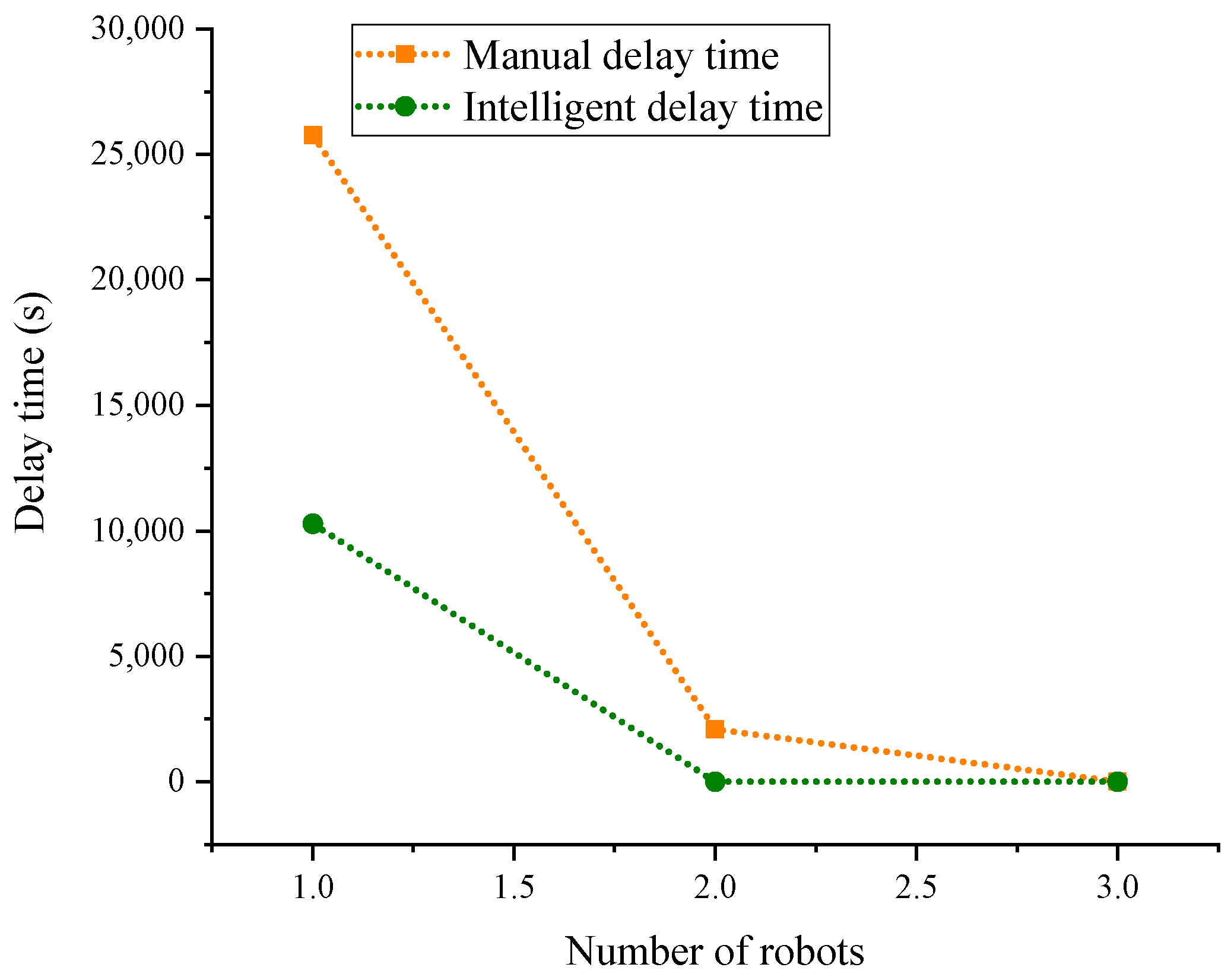When a single robot performs delivery, as shown in Figure 15, there are 5 delivery delay task lists (task list 2, task list 3, task list 8, task list 6, task list 9), and the delay time is 15,194 s. Compared with manual scheduling, the delay time is reduced by 3.7%. According to the calculated data, the relationship between the delay time and the number of robots under different scheduling modes is drawn (Figure 16). It can be seen from the Figure that under the same delay condition, more robots are needed to complete the task list manually; when the number of robots is the same, manual scheduling takes longer to complete the task list.

In the actual scheduling application, because the task list information is constantly updated and the real-time performance is strong, the scheduling scheme is also constantly updated and transformed. In the solution process, the accuracy of the scheduling scheme is at the expense of the solution time. The solution time is an important index that affects the engineering application of the algorithm. We hope that the process of obtaining the scheduling scheme is fast and efficient. Statistics dual-layer genetic algorithm to solve the time 20 times, draw a scatter diagram as shown in Figure 17, can be seen from the Figure, the solution time is more evenly distributed in the vicinity of 10 s, take the average of 9.7 s.

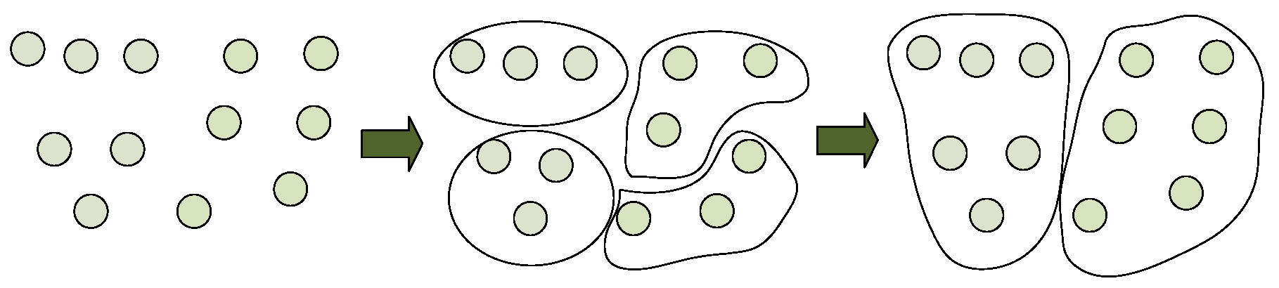
6. Working Face Spatiotemporal Clustering Based on Hierarchical Clustering

Working face clustering solution can reduce the solution time, to ensure efficient path planning methods. Hierarchical clustering is a clustering algorithm that creates a hierarchical nested clustering tree by calculating the similarity between data points in different categories. In a clustering tree, the original data points of different categories are the lowest layer of the tree, and the top layer of the tree is a clustering root node. There are two methods to create clustering trees: bottom-up merging and top-down splitting. In this paper, a bottom-up merging algorithm is used to cluster the output hierarchical structure, which is more informative than the unstructured clustering set returned by planar clustering. The hierarchical clustering algorithm is traditionally based on Single Linkage, Complete Linkage, and Average Linkage to calculate the similarity of data. The Single Linkage and Complete Linkage methods are easily affected by extreme values. Based on the traditional hierarchical clustering algorithm, this paper designs a time-space data conversion coefficient ω based on the coordinates of the working face and the required delivery time of the working face. The Average Linkage formula is used to cluster the spatiotemporal data, and the working face is clustered together according to its similarity, as shown in Figure 18.

Taking $\omega =\frac{{\mathrm{d}}_{ij}}{{\mathrm{s}}_i}=v=1$, it is proved that if the robot starts from the industrial square and arrives at the working face i at the required time, then ${\mathrm{d}}_{ij}={\mathrm{d}}_{0i}$, ${\mathrm{s}}_i={\mathrm{t}}_{0i}$, $\frac{{\mathrm{d}}_{0j}}{{\mathrm{t}}_{0i}}=v$.

Use the Average Linkage formula to calculate the distance from data points (A, F) to (B, C):

$$\mathrm{D}=\frac{\left\{\sqrt{{\left(A-B\right)}^2}+\sqrt{{\left(A-C\right)}^2}+\sqrt{{\left(F-B\right)}^2}+\sqrt{{\left(F-C\right)}^2}\right\}}{4}$$

(20)

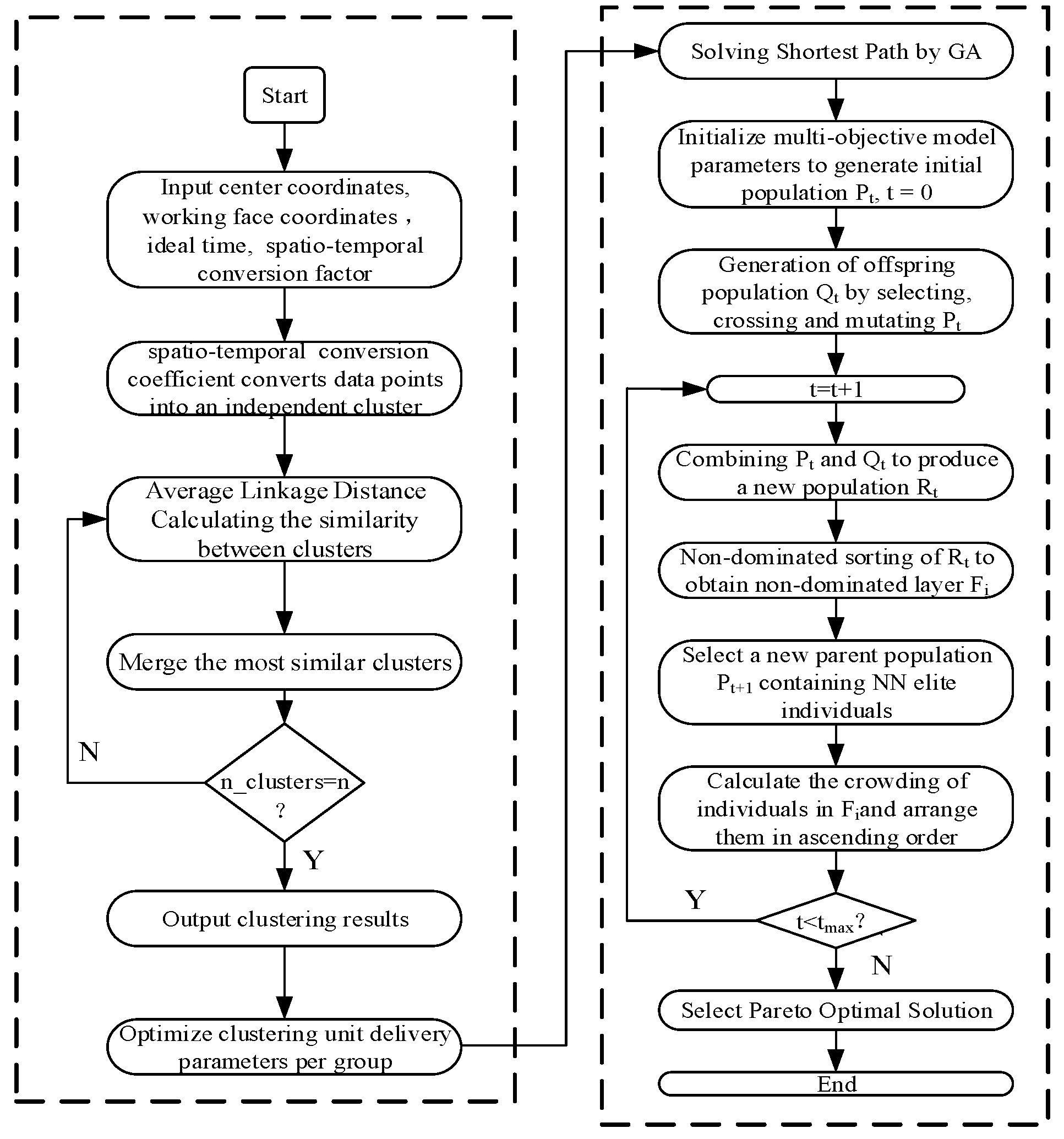
The overall process of intelligent scheduling strategy based on hierarchical clustering dual-layer genetic algorithm is shown in Figure 19. First, input the initial parameters of the distribution, including the distribution center coordinates, working face coordinates, expected delivery time, and spatiotemporal conversion coefficient; then, the data are normalized by using the spatiotemporal conversion coefficient, and the spatial two-dimensional coordinates and the time one-dimensional coordinates are regarded as three-dimensional data points. Each data point is an independent cluster; finally, the Average Linkage formula is used to calculate the similarity between clusters, and the clusters with the highest similarity are merged until the cluster category is consistent with the set parameter n, and the clustering result is output. The distribution parameters are optimized inside the clustering unit. Firstly, the basic genetic algorithm is used to solve the shortest path inside the unit. Then, the NSGA-II framework is used to solve the minimum robot and the shortest delay time dual-objective model, and the population P_t is initialized. The selection, crossover, and mutation operations are performed on P_t to generate the offspring population Q_t. The P_t and Q_t are merged to generate a new population R_t. The non-dominated sorting is performed on R_t to obtain the non-dominated layer F_i. The new parent population P_t+1 containing NN elite individuals is selected to calculate the crowding degree of individuals in Fi and arrange them in ascending order. Finally, when the number of iterations reaches the set value, the Pareto optimal solution is selected. Output delivery path parameters.

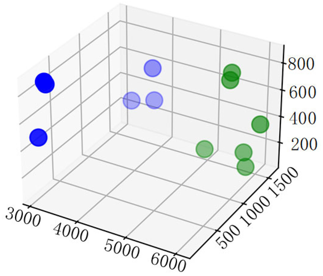
Set the number of categories n = 2, and use hierarchical clustering to cluster task lists. The results are shown in Figure 20. The blue dots represent task list 1, task list 2, task list 3, task list 6, task list 8, and task list 9 as a group. The green dots represent task list 4, task list 5, task list 7, task list 10, task list 11, and task list 12 as a group. The intelligent scheduling algorithm is used to solve each group of task lists, respectively. 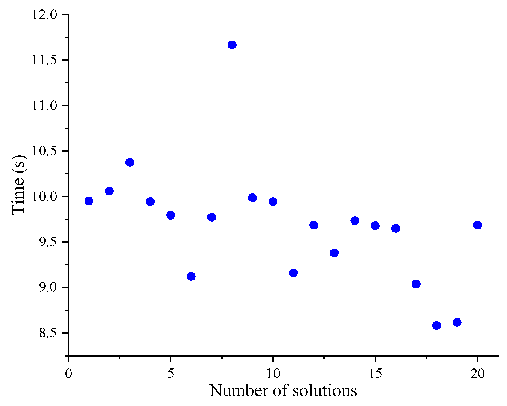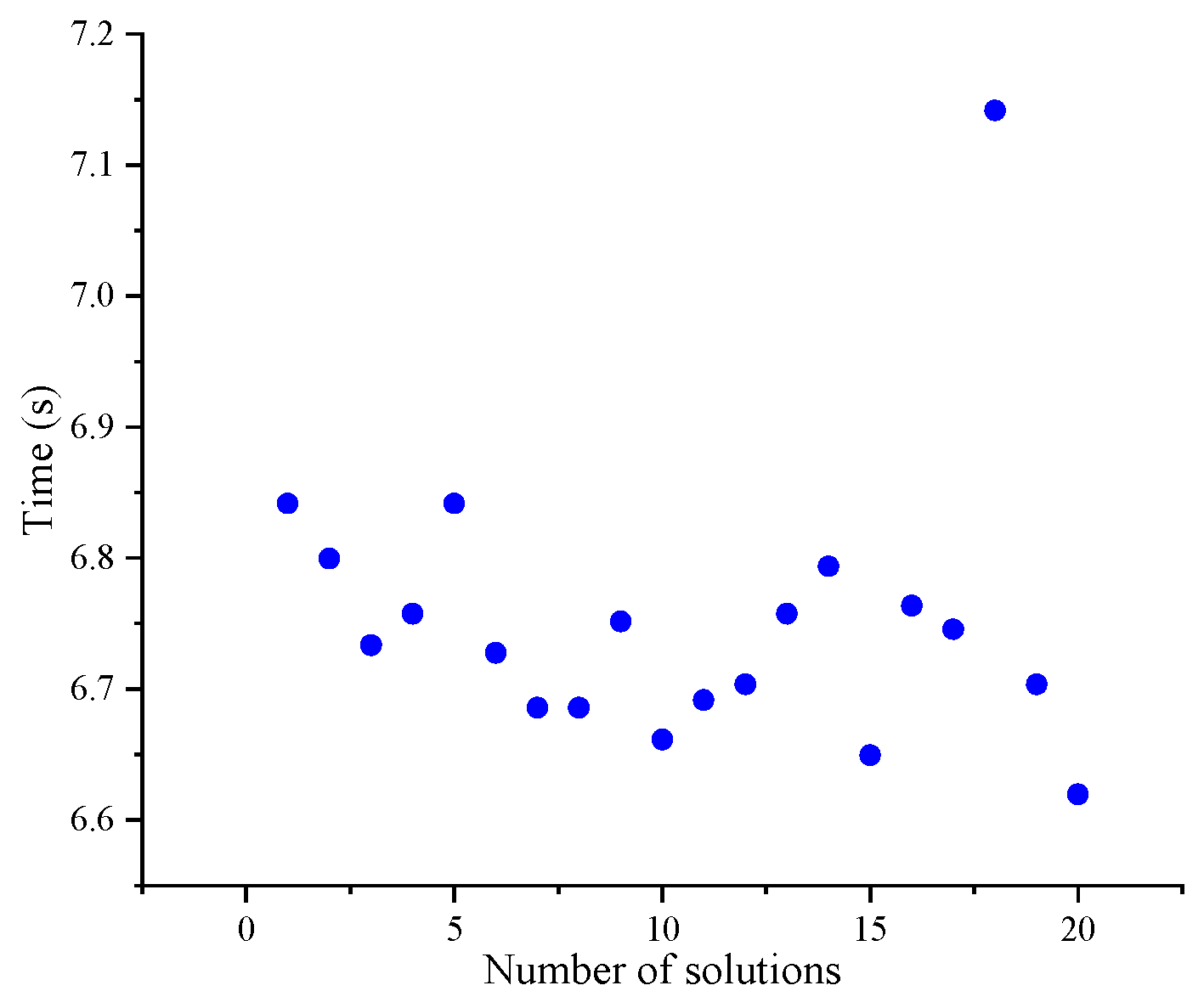The solution path planning is shown in Figure 21, and the result is consistent with the result of the non-grouping solution. The 20 times solution time in the group of dual-layer genetic algorithm based on hierarchical clustering is counted, and the scatter diagram is drawn as shown in Figure 22. It can be seen from the diagram that the solution time is evenly distributed in the vicinity of 6.7~6.9 s, with an average value of 6.8 s. Compared with the dual-layer genetic algorithm, the solution time is reduced by 30%. In the actual distribution, the task list information is always updated in real time, so each time, one only needs to pay attention to the first set of results of the delivery time.

7. Conclusions

In an attempt to solve the problems of the low intelligent distribution degree and high working intensity of auxiliary transportation systems, an intelligent distribution strategy of coal mine auxiliary transportation materials is proposed based on the application of the unmanned driving technology of auxiliary transportation robots. Firstly, combined with the characteristics of materials and standard containers, a three-dimensional loading model is established with the goal of maximizing the space utilization of standard containers. The three-dimensional space segmentation heuristic algorithm is used to solve the material loading scheme. Compared with manual random loading, the maximum space utilization of standard containers increases by 18%, and the standard container occupancy decreases by 20%. Then, the multi-objective optimization model of distribution parameters is established with the shortest distribution distance, the shortest delay time, and the least distribution vehicles as the objectives, and the dual-layer genetic algorithm is used to solve the distribution scheme. The results show that in the case of having 2 robots available, compared with manual scheduling, the total distribution distance is reduced by 34% and the delay time is reduced by 100%, which has better performance. Finally, the spatiotemporal conversion coefficient is designed to solve the task list by hierarchical clustering, and the solution time is reduced by 30%, which improves the efficiency of real-time task list dynamic programming.

There are many kinds of materials and different forms in the distribution of auxiliary transportation systems. This paper mainly takes rectangular materials as the research object, and the next step is to study the combination loading method of round materials, such as oil and air ducts and rectangular materials. In addition, the dual-layer genetic algorithm based on hierarchical clustering is insufficient for the analysis of engineering applicability, such as robot failure, traffic congestion, and roof collapse. The decision-making results of the algorithm are still unknown and still need to be explored.