Coal Gangue Recognition during Coal Preparation Using an Adaptive Boosting Algorithm

Abstract

The recognition of coal and gangue is the premise and foundation of coal gangue intelligent sorting. Adaptive boosting (AdaBoost) algorithm-based coal gangue identification has not been studied in depth. This paper proposed a coal gangue image recognition algorithm and a strong classifier based on the AdaBoost algorithm with a genetic algorithm (GA)-optimized support vector machine (SVM). One thousand coal gangue images were collected on-site and expanded to five thousand via rotation and exposure adjustment. The 12 gray-level gradient co-occurrence matrix texture features of the images were extracted to construct a feature vector, establishing the training dataset and test dataset. Selection of the SVM kernel function, the GA optimization parameter setting, and the base classifier number was discussed. The coal gangue image recognition effects of the AdaB-GA-SVM classifier and the other strong classifiers with different base SVM classifiers were investigated. The results indicated that the recognition accuracy of GA-SVM was the best when the kernel function of SVM was RBF and the population number, crossover probability, and mutation probability were 80, 0.9, and 0.005, respectively. The AdaB-GA-SVM classifier has excellent identification and effective classification performance with the highest accuracy of 95%, a precision rate of 92.8%, recall rate of 97.3%, and KS values of 0.79.

1. Introduction

Gangue sorting is one of the crucial processes in coal preparation because raw coal is mixed with gangue impurities during production. A gangue has a low calorific value and releases toxic gases, such as SO₂, CO, CO_2, and NO_x, when burned, which results in coal quality reduction and environmental pollution, affecting the clean and efficient use of coal [1]. The existing coal gangue sorting methods mainly involve manual and mechanical sorting. 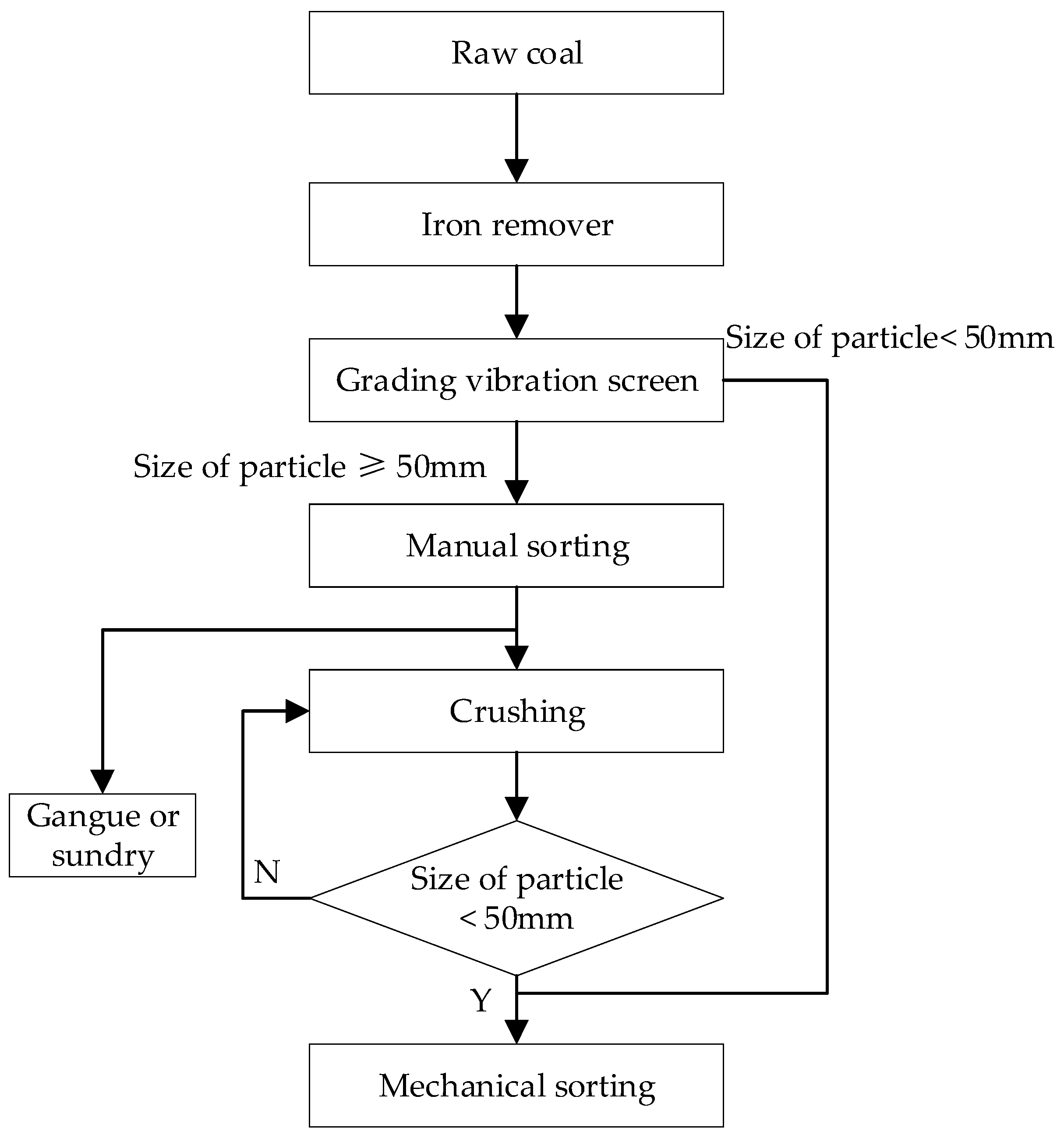As shown in Figure 1, when the raw coal flow flows into the raw coal preparation workshop, the iron and sundries in the raw coal flow are removed through the iron remover, and then enter the raw coal classification screen for screening. Those with particle sizes of less than 50 mm directly enter the mechanical separation operation. Those with particle sizes of more than 50 mm are manually selected to remove part of the sundries in the coal and visible gangue, and then broken into qualified particle sizes (less than 50 mm), and further separation is carried out using other mechanical separation methods such as a moving screen jig. 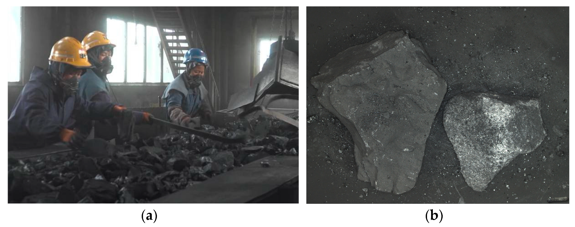When manually sorting gangue, illustrated in Figure 2, the workers judge the gangue in the coal flow through the naked eye and pick it out by hand. The labor intensity is high, the working environment is bad, the workers can very easily inhale fine particles (although wearing protective masks) and can easily be injured by the high-speed belt or scraper conveyor, seriously affecting the health of the workers and posing great potential safety risks [2]. To keep the sorting workers away from the harsh working environment, intelligent coal gangue sorting equipment, especially coal gangue sorting robots, has received considerable attention in the industry [3,4,5,6]. Coal gangue recognition is the foundation of its intelligent sorting and is a crucial coal gangue sorting robot technology.

The investigations on coal gangue identification can be traced back to the 1960s with more than 10 identification methods, such as the γ-ray, X-ray, photoelectric, and infrared methods [7,8,9,10,11]. Despite numerous accomplishments, these methods have bottlenecks, such as limited application occasions, radiation hazards, and low recognition accuracy. With the development of image processing technology and machine learning, coal gangue identification methods have shifted their focus onto coal gangue image recognition. Wang, Li, and Yang [12] investigated coal gangue response characteristics under different illuminations and used a SVM classifier to realize the identification of coal and gangue. Zhao et al. [13] constructed a PSO-SVM model to recognize coal and gangue. Su et al. [14] and Pu et al. [15] introduced transfer learning for the identification of coal and gangue based on a convolutional neural network (CNN). Li et al. [16] proposed a hierarchical framework for coal gangue detection based on CNNs. McCoy and Auret [17] reviewed the machine learning applications in mineral processing. Hou [18] established a coal gangue separation system based on the difference between coal and gangue in their surface textures and grayscale features, and proposed a method of combining image feature extraction and a feed-forward artificial neural network.

Alfarzaeai et al. [19] addressed the topic of coal gangue recognition. They created a new model called CGR-CNN based on CNN using thermal images as standard images for coal gangue recognition. Lei et al. [3] constructed a visual depth neural network fast coal classification net (FCCN) based on CNN, and implemented a visual coal classification detection algorithm for coal gangue sorting robots. Liu, Li, et al. [1] studied coal gangue detection based on enhanced YOLOv4. Li et al. [20] conducted research on a coal gangue detection and recognition algorithm based on deformable convolution YOLOv3 (DCN-YOLOv3). Yan et al. [21] studied an intelligent classification method of coal gangue based on multispectral imaging technology and target detection by the YOLOv5.1. In the coal preparation streamline, the state of gangue in raw coal flow is diverse, such as exposing outside coal, being partially or fully covered by pulverized coal. Furthermore, extracting the features of a coal gangue image is challenging due to the harsh site conditions of low illumination and high dust. The present coal gangue recognition methods in the literature have limited applications. Therefore, further study is required for the segmentation, enhancement, feature extraction, and recognition of a coal gangue image. A coal gangue recognition algorithm based on deep learning does not need to consider the extracted features. Still, the classifier’s training needs a large number of marked samples and a large amount of calculation; thus, the requirements for lightweight and real-time performance pose a significant challenge to its field application. Li et al. [22] investigated the effects of illuminance and external moisture on grayscale and texture features of coal and gangue images, which provided an essential guide for the image-based identification of coal and gangue under working conditions. Li and Gong [23] studied a preprocessing model for low-quality images of coal and gangue based on a bilateral filtering joint enhancement algorithm.

Above all, literature investigations on coal gangue recognition have been extensively conducted, but a practical solution has not yet been satisfactorily provided. Wang, Li, and Yang [12] and Li et al. [4] have studied the coal gangue recognition model based on a support vector machine (SVM). Still, low accuracy and insufficient robustness problems were caused by its insensitivity to noise and difficult parameter adjustment. There are few studies on the use of integrated algorithms to improve the accuracy of SVM coal gangue classification.

Therefore, the novel contributions of this paper are as follows:

• Aiming at the shortcomings of the SVM classifier for coal gangue recognition, this paper used a genetic optimization algorithm to improve its noise insensitivity and difficult parameter adjustment, used an adaptive boosting (AdaBoost) algorithm to enhance its recognition accuracy, and constructed a coal gangue recognition and classification model;
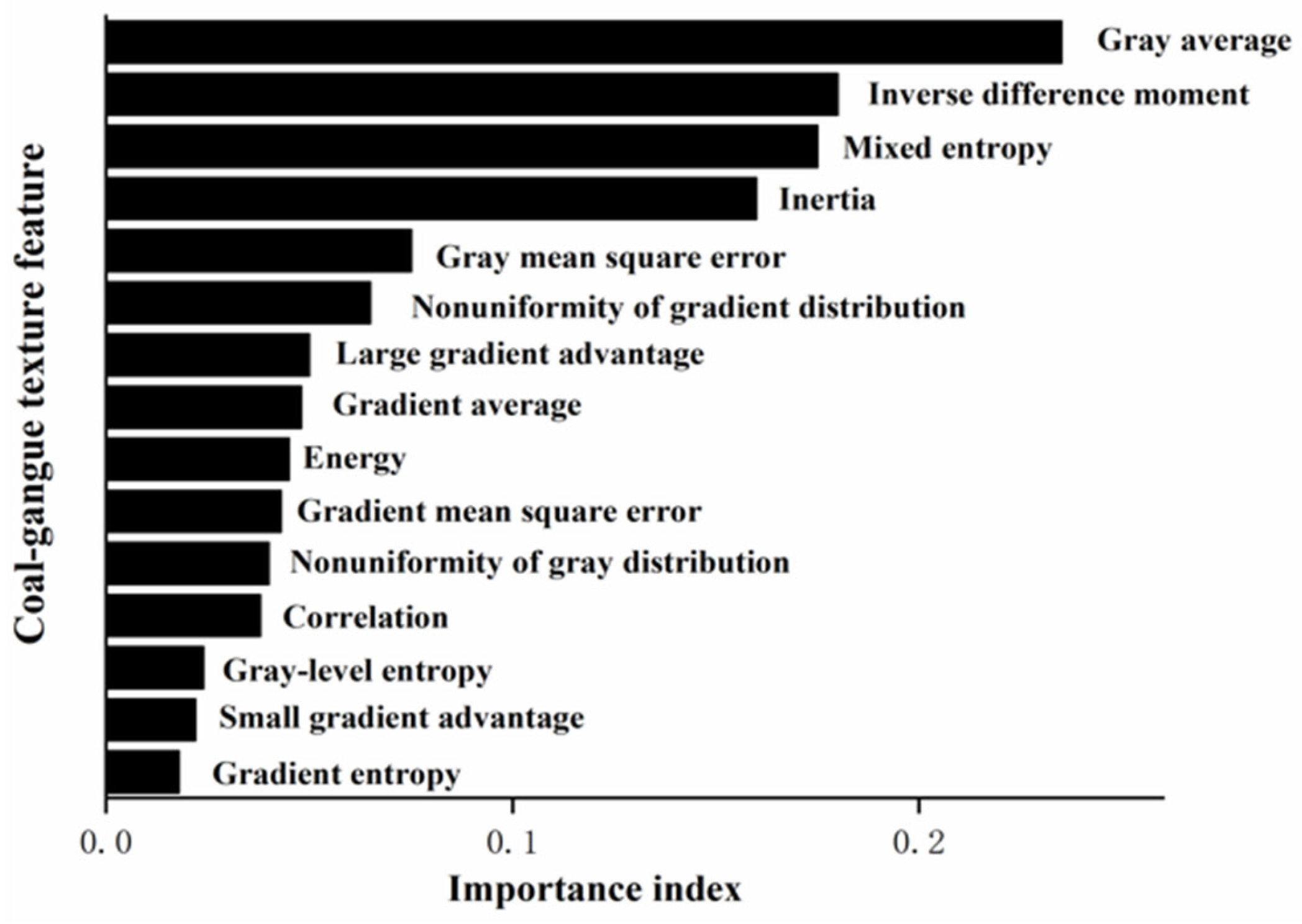
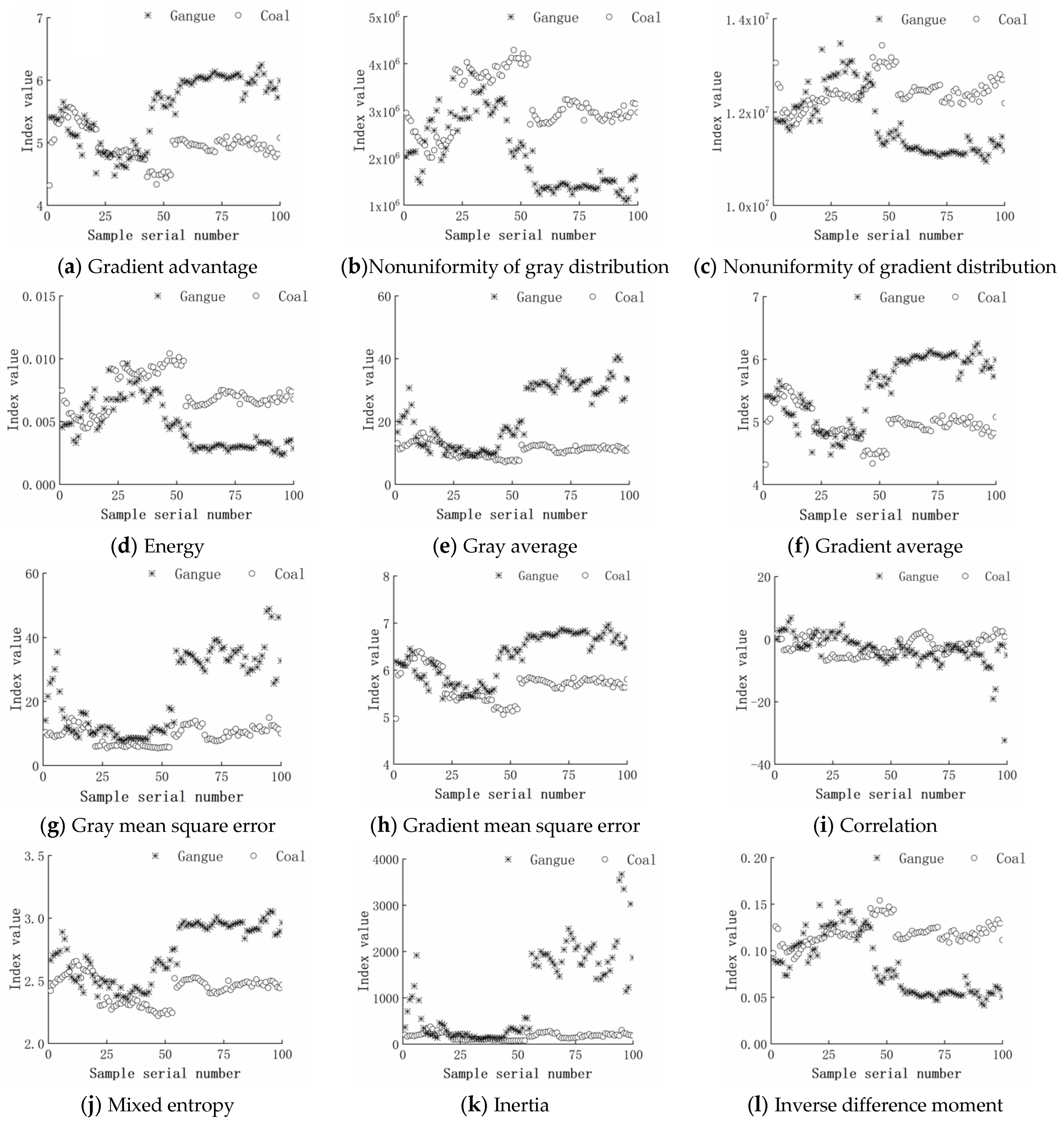
• The indices of GGCM were introduced to characterize the features of the coal and gangue and a coal-gangue sample dataset was constructed with the coal and gangue images obtained by experiment and on-site to verify the performance of the proposed algorithm.

2. Principle and Theory

This section presents the proposed method and its algorithm. This study used an SVM classifier as the AdaBoost integration base classifier, and a genetic algorithm (GA) was employed to optimize the SVM parameters.

2.1. SVM Algorithm and SVM Classifier

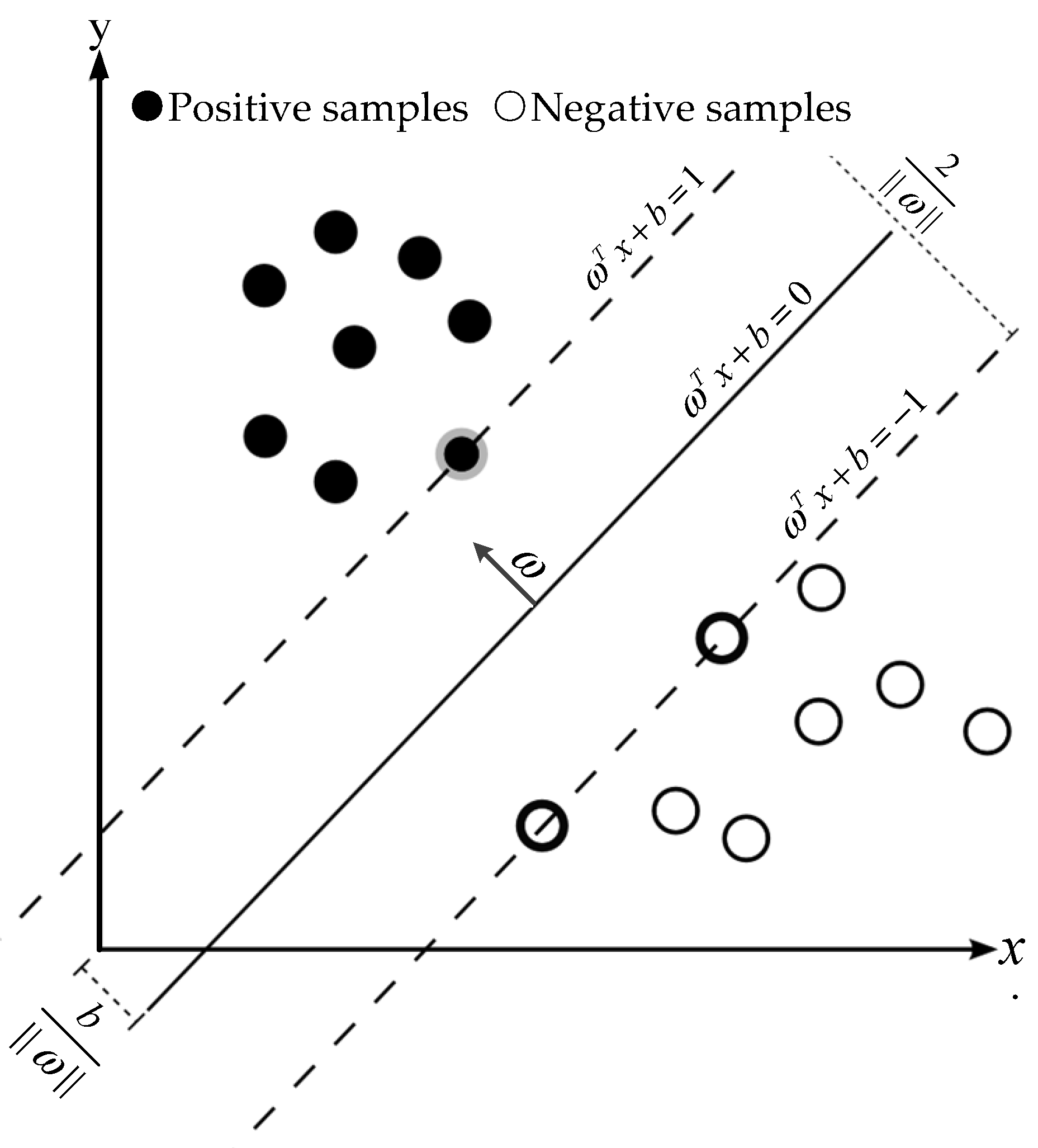
SVM is a machine learning method based on a statistical theory proposed by Vapnik and Chervonenkis [24]. It is widely used in text classification, handwritten character recognition, and image classification owing to its excellent generalization performance and ability to process high-dimensional data. The fundamental principle is to find an optimal hyperplane that can meet the classification requirements and which has the most considerable interval, as presented in Figure 3.

Let D = {(x_i, y_i), i = 1, 2, …, N, x ∈ R, y ∈ (−1,1)}, x_i is the sample data to be classified, and y_i is the label of the data x_i. The classification plane (ω, b) can be described using the following linear equation:

$${\omega }^{T}gx+b=0$$

(1)

where ω denotes the normal vector to the classification plane, and b indicates the displacement term. For any sample in the linearly separable sample set, there are

$$\{\begin{array}{c}{y}_i=+1, {\omega }^T{x}_i+b\ge +1\\ y_i=-1, {\omega }^T{x}_i+b<+1\end{array}$$

(2)

Equation (2) can be abbreviated as

$$y_i\left({\omega }^T{x}_i+b\right)\ge 1$$

(3)

In all the vectors ω, there is a vector whose distance from the classification plane is the smallest and satisfies the equal sign of Equation (2), which is called the support vector. The sum of the distances γ from all the support vectors to the hyperplane is

$$\gamma =\frac{2}{\Vert \omega \Vert }$$

(4)

The hyperplane with the largest distance γ is the optimal hyperplane. Then, the classification problem is transformed into the problem of finding the optimal hyperplane, namely, finding the optimal parameters ω and b in Equation (1) under constraints

$$\begin{array}{cc}\underset{\omega ,b}{\max }\frac{2}{\Vert \omega \Vert }\hfill & \\ \mathrm{s}.\mathrm{t}. y_i({\omega }^T{x}_i\hfill & +b)\ge 1,i=1,2,\dots ,N\hfill \end{array}$$

(5)

or:

$$\begin{array}{cc}\underset{\omega ,b}{\min }\frac{1}{2}\Vert \omega \Vert \hfill & \\ \mathrm{s}.\mathrm{t}. y_i\left({\omega }^T{x}_i+b\right)\ge 1,i=1,2,\dots ,N\hfill \end{array}$$

(6)

For calculation convenience, remove the root sign in Equation (6), then

$$\begin{array}{cc}\underset{\omega ,b}{\min }\frac{1}{2}{\Vert \omega \Vert }^2\hfill & \\ \mathrm{s}.\mathrm{t}. y_i\left({\omega }^T{x}_i+b\right)\ge 1, i=1,2,\dots ,N\hfill \end{array}$$

(7)

If the Lagrange function is introduced into the above formula, there is

$$L\left(\omega ,b,\alpha \right)=\frac{1}{2}{\Vert \omega \Vert }^2+{\displaystyle \mathsf{\sum }}_{i=1}^N{\alpha }_i\left(1-y_i\left({\omega }^T{x}_i+b\right)\right)$$

(8)

where the Lagrange multiplier α_i ≥ 0. Then, the problem of finding the optimal classification plane comes down to solving

$$\begin{array}{c}\underset{\alpha }{\max }\left({\displaystyle {\displaystyle \mathsf{\sum }}_{i=1}^N}{\alpha }_i-\frac{1}{2}{\displaystyle {\displaystyle \mathsf{\sum }}_{i=1}^N}{\displaystyle {\displaystyle \mathsf{\sum }}_{j=1}^N}{\alpha }_i{\alpha }_j{y}_i{y}_j{x}_i{}^T{x}_j\right)\\ s.t. 0\le {\alpha }_i, {\displaystyle {\displaystyle \mathsf{\sum }}_{i=1}^N}{\alpha }_i{y}_i=0,i=1,2,\dots ,N\end{array}$$

(9)

For the nonlinear classification problem, the kernel function of K(x_i, x_j) is introduced, and the classification problem is reduced to

$$\begin{array}{c}\underset{\alpha }{\max }\left({\displaystyle {\displaystyle \mathsf{\sum }}_{i=1}^N}{\alpha }_i-\frac{1}{2}{\displaystyle {\displaystyle \mathsf{\sum }}_{i=1}^N}{\displaystyle {\displaystyle \mathsf{\sum }}_{j=1}^N}{\alpha }_i{\alpha }_j{y}_i{y}_{j}K\left({\mathit{x}}_i,{\mathit{x}}_j\right)\right)\\ s.t. 0\le {\alpha }_i\le C,{\displaystyle {\displaystyle \mathsf{\sum }}_{i=1}^m}{\alpha }_i{y}_i=0,i=1,2,\dots ,N\end{array}$$

(10)

where C denotes the penalty factor. The final classification discriminant function is defined as

$$f\left(x\right)=\mathit{sgn}\left({\displaystyle \mathsf{\sum }}_{i=1}^N{a}_i{y}_{i}K\left({\mathit{x}}_i,{\mathit{x}}_j\right)+b\right)$$

(11)

where sgn(x) is the sign discrimination function. When x > 0, it returns 1; otherwise, it returns 0.

The loss function of SVM is an unbounded convex function, resulting in the same penalty on classification error samples, and exceptionally susceptible to noise while ensuring the confidence of the classification results. In addition, SVM has parameter sensitivity, complex parameter tuning, and unstable classification accuracy. The coal gangue recognition model based on the basic SVM algorithm lacks accuracy and robustness, impacting the effect of the algorithm on coal gangue recognition.

2.2. GA Optimization and SVM Base Classifier Construction

The introduction of parameter optimization algorithms, such as the GA algorithm [25], particle swarm optimization (PSO) algorithm [26], and ant colony algorithm [27], can adaptively search the global optimization and effectively reduce the difficulty of the parameter tuning of the SVM model. This paper introduced GA into the SVM algorithm to optimize the penalty factor and kernel function parameters, and the GA-SVM model was created.

GA is a method for searching for the optimal solution by simulating the natural evolutionary process. This algorithm converts problem-solving into a process that is similar to the crossover and mutation of chromosomal genes in biological evolution. Owing to its strong robustness, it is widely used in combination optimization, machine learning, signal processing, adaptive control, and artificial life. The optimization process of the GA is as follows:

• Set the evolutionary iteration counter t = 0, the maximum evolutionary iteration T, and randomly generate M individuals as the initial population P(0);
• Calculate the fitness of each individual in the population P(t);
• Obtain the next generation’s population P(t + 1) through selection, crossover, and mutation of population P(t);
• Judge whether the termination condition is reached. If t < T, repeat Step 3; else, if t = T, terminate the evolution;
• Take the individual with the greatest fitness obtained in the evolution process as the optimal solution, and the SVM base classifier is constructed using the optimal parameters.

2.3. ADAB-GA-SVM Classifier Construction

The AdaBoost algorithm was employed to obtain a strong classifier model to improve the anti-noise performance of the SVM algorithm, referred to as the AdaB-GA-SVM model. AdaBoost is the most representative boosting tree algorithm proposed based on Boosting by Freund and Schapire [28]. The AdaBoost tree algorithm is widely used for classification in various fields as it can keep the training between classifiers unaffected to ensure structural stability and maximize model generality. Dou, Chen, and Yue [29] proposed a multi-classification algorithm based on AdaBoost, which exhibited an excellent remote sensing image classification performance. Zhang et al. [30] employed the AdaBoost algorithm to integrate the SVM base classifier into strong classifiers to achieve higher classification accuracy in different dataset sizes. The AdaBoost algorithm flow is as follows:

(1)

Initialize the weight of the sample set D.

$${\omega }_i^1=\raisebox{1ex}{$1$}\!\left/ \!\raisebox{-1ex}{$N$}\right.\begin{array}{cc},& i=1,2,\cdots ,N\end{array}$$

(12)

(2)

Let the iteration number be M, for t = 1, 2, …, M:

• Train the GA-SVM classifier using the sample set D with weight ω_i^t and obtain a base classifier f_t(x);
• Calculate the classification error rate e_t and weight of the classifier λ_t:

  $$e_t={\displaystyle \mathsf{\sum }}_{i=1}^N{\omega }_i^t\cdot I\left(y_i\ne f_t\left(x_i\right)\right)$$

  (13)

  $${\lambda }_t=\frac{1}{2}\ln (\frac{1-e_t}{e_t})$$

  (14)

  where I (y_i ≠ f_t(x_i)) is a discriminant function, which returns 1 when the prediction result of the base classifier f_t(x) is inconsistent with the sample label y_i; otherwise, it returns 0.
• Update the weight of the training set sample to ω_i^t+1 according to the prediction result of the base classifier f_t(x):

  $${\omega }_i^{t+1}=\{\begin{array}{c}\frac{{\omega }_i^t\exp (-{\lambda }_t)}{{\displaystyle {{\displaystyle \mathsf{\sum }}}_{i=1}^N}{\omega }_i^t\exp (-{\lambda }_t)} f_t\left(x_i\right)=y_i\\ \frac{{\omega }_i^t\exp ({\lambda }_t)}{{\displaystyle {{\displaystyle \mathsf{\sum }}}_{i=1}^N}{\omega }_i^t\exp ({\lambda }_t)} f_t\left(x_i\right)\ne y_i\end{array}$$

  (15)

(3)

Build the final strong classifier as

$$F\left(x\right)={\displaystyle \mathsf{\sum }}_{t=1}^M{\lambda }_t{f}_t\left(x\right)=F_{M-1}\left(x\right)+{\lambda }_M{f}_M\left(x\right)$$

(16)

Generally, the step size and maximum number of iterations are used together to determine the fitting effect of the AdaBoost algorithm, and the constructed strong classifier is given by the following equation:

$$F\left(x\right)=F_{M-1}\left(x\right)+\nu {\lambda }_M{f}_M\left(x\right)$$

(17)

where ν denotes the learning rate, 0 < ν ≤ 1. The classification discriminant function g(x) is defined as

$$g\left(x\right)=\mathit{sgn}\left( F\left(x\right)\right)$$

(18)

where sgn(x) is the same as Equation (11).

3. Materials and Methods

3.1. Coal and Gangue Image Collection and Preprocessing

The coal gangue image samples were collected from the Wuyuan Coal preparation plant. Considering the impact of environmental factors, such as light and coal dust, on the quality of the collected coal-gangue image, the coal gangue image data were collected at different periods to increase the model’s generalization performance.

After the screening, cutting, and labeling of the coal and the gangue images collected on-site, 500 images of the coal and the gangue were individually obtained, comprising a total of 1000 sample data. A total of 800 data were selected as the training set and the remaining 200 as the test set. During selection, the proportion of the coal gangue images was controlled at 1:1 to keep the coal gangue sample data balanced. The training and test sets were expanded to 4000 and 1000, respectively, through left–right rotation and exposure adjustment, to enrich the dataset.

The coal gangue images were preprocessed by gray conversion, gamma function correction, and image enhancement. After preprocessing, the gray-level of each coal-gangue image was 256, the size was 2000 × 2000, and the format was PNG. Figure 4 demonstrates the effect comparison of the coal gangue images before and after preprocessing.

3.2. Gray-Level Gradient Co-Occurrence Matrix Texture Feature Extraction

The gray-level co-occurrence matrix (GLCM) is a matrix function of image pixel distance and angle. It reflects the comprehensive information of an image in direction, adjacent interval, and change range through the correlation between the gray levels of two pixels with a certain distance and direction in the image [31]. The generation principle is described as follows. Starting from the pixel point (x, y) of the gray value i, move a certain distance δ at an angle θ along the matrix construction direction toward the pixel point (x + Δx, y + Δy) of the gray value j, as presented in Figure 5, and calculate the number of pixel pairs with the relative position relationship in the whole image to obtain the joint probability distribution P(i, j) of pixel pair (i, j); construct a square matrix with the joint probability distribution P(i, j) of all pixel pairs (i, j), then normalize the square matrix by the total number of (i, j) combination, and finally obtain the GLCM. Δx and Δy are determined by spacing δ and angle θ, and θ indicates the generation direction of GLCM.

The addition of the gradient information of the image to the GLCM constitutes the GGCM, which can contain the texture primitives and their arrangement information. This reflects the relationship between the gray-level and the image pixel point gradient (or edge). The gray-level of each pixel is the basis of an image, and the gradient is the element of the image edge contour [32]. The GGCM is expressed as follows:

$$\left\{H\left(x,y\right); x=0,1,\mathrm{\dots }{L}_f-1; y=0,1,\mathrm{\dots },L_g-1\right\}$$

(19)

where H(x, y) is the element of the GGCM, representing the number of pixels with grayscale x in the normalized grayscale image F(i, j) and gradient y in the normalized gradient image G(i, j); L_f, the maximum gray-level of the grayscale image; and L_g, the maximum gradient level of the gradient image. The GGCM is normalized as follows:

$$\widehat{H}\left(x,y\right)=\frac{H\left(x,y\right)}{{\displaystyle {{\displaystyle \mathsf{\sum }}}_{x=0}^{L_f-1}}{\displaystyle {{\displaystyle \mathsf{\sum }}}_{y=0}^{L_g-1}}H\left(x,y\right)}$$

(20)

Based on the normalized GGCM $\widehat{H}\left(x,y\right)$, the 15 grayscale gradient texture features of the coal gangue image can be extracted using the formula in

Table A1. The 15 grayscale gradient texture features and their calculation formulas.

No.	Texture Feature	Calculation Formula
1	large gradient advantage	$T_1={\displaystyle {\displaystyle \mathsf{\sum }}_{x=0}^{L_f-1}}{\displaystyle {\displaystyle \mathsf{\sum }}_{y=0}^{L_g-1}}{y}^2\widehat{H}\left(x,y\right)/{\displaystyle {\displaystyle \mathsf{\sum }}_{x=0}^{L_f-1}}{\displaystyle {\displaystyle \mathsf{\sum }}_{y=0}^{L_g-1}}\widehat{H}\left(x,y\right)$
2	small gradient advantage	$T_2={\displaystyle {\displaystyle \mathsf{\sum }}_{x=0}^{L_f-1}}{\displaystyle {\displaystyle \mathsf{\sum }}_{y=0}^{L_g-1}}\frac{\widehat{H}\left(x,y\right)}{{\left(y+1\right)}^2}/{\displaystyle {\displaystyle \mathsf{\sum }}_{x=0}^{L_f-1}}{\displaystyle {\displaystyle \mathsf{\sum }}_{y=0}^{L_g-1}}\widehat{H}\left(x,y\right)$
3	gray distribution nonuniformity	$T_3={\displaystyle {\displaystyle \mathsf{\sum }}_{x=0}^{L_f-1}}{\left[{\displaystyle {\displaystyle \mathsf{\sum }}_{y=0}^{L_g-1}}\widehat{H}\left(x,y\right)\right]}^2/{\displaystyle {\displaystyle \mathsf{\sum }}_{x=0}^{L_f-1}}{\displaystyle {\displaystyle \mathsf{\sum }}_{y=0}^{L_g-1}}\widehat{H}\left(x,y\right)$
4	gradient distribution nonuniformity	$T_4={\displaystyle {\displaystyle \mathsf{\sum }}_{x=0}^{L_g-1}}{\left[{\displaystyle {\displaystyle \mathsf{\sum }}_{y=0}^{L_f-1}}\widehat{H}\left(x,y\right)\right]}^2/{\displaystyle {\displaystyle \mathsf{\sum }}_{x=0}^{L_f-1}}{\displaystyle {\displaystyle \mathsf{\sum }}_{y=0}^{L_g-1}}\widehat{H}\left(x,y\right)$
5	energy	$T_5={\displaystyle {\displaystyle \mathsf{\sum }}_{x=0}^{L_f-1}}{\displaystyle {\displaystyle \mathsf{\sum }}_{y=0}^{L_g-1}}{\widehat{H}}^2\left(x,y\right)$
6	gray average	$T_6={\displaystyle {\displaystyle \mathsf{\sum }}_{x=0}^{L_f-1}}x{\displaystyle {\displaystyle \mathsf{\sum }}_{y=0}^{L_g-1}}\widehat{H}\left(x,y\right)$
7	gradient average	$T_7={\displaystyle {\displaystyle \mathsf{\sum }}_{y=0}^{L_g-1}}y{\displaystyle {\displaystyle \mathsf{\sum }}_{x=0}^{L_f-1}}\widehat{H}\left(x,y\right)$
8	gray mean square error	$T_8={\left[{\displaystyle {\displaystyle \mathsf{\sum }}_{x=0}^{L_f-1}}{\left(x-T_6\right)}^2{\displaystyle {\displaystyle \mathsf{\sum }}_{y=0}^{L_g-1}}\widehat{H}\left(x,y\right)\right]}^{\frac{1}{2}}$
9	gradient mean square error	$T_9={\left[{\displaystyle {\displaystyle \mathsf{\sum }}_{y=0}^{L_g-1}}{\left(y-T_7\right)}^2{\displaystyle {\displaystyle \mathsf{\sum }}_{x=0}^{L_f-1}}\widehat{H}\left(x,y\right)\right]}^{\frac{1}{2}}$
10	correlation	$T_{10}={\displaystyle {\displaystyle \mathsf{\sum }}_{x=0}^{L_f-1}}{\displaystyle {\displaystyle \mathsf{\sum }}_{y=0}^{L_g-1}}\left(x-T_6\right)\left(y-T_7\right)\widehat{H}\left(x,y\right)$
11	gray-level entropy	$T_{11}=-{\displaystyle {\displaystyle \mathsf{\sum }}_{x=0}^{L_f-1}}{\displaystyle {\displaystyle \mathsf{\sum }}_{y=0}^{L_g-1}}\widehat{H}\left(x,y\right)\log {\displaystyle {\displaystyle \mathsf{\sum }}_{y=0}^{L_g-1}}\widehat{H}\left(x,y\right)$
12	gradient entropy	$T_{12}=-{\displaystyle {\displaystyle \mathsf{\sum }}_{x=0}^{L_f-1}}{\displaystyle {\displaystyle \mathsf{\sum }}_{y=0}^{L_g-1}}\widehat{H}\left(x,y\right)\log {\displaystyle {\displaystyle \mathsf{\sum }}_{x=0}^{L_f-1}}\widehat{H}\left(x,y\right)$
13	mixed entropy	$T_{13}=-{\displaystyle {\displaystyle \mathsf{\sum }}_{x=0}^{L_f-1}}{\displaystyle {\displaystyle \mathsf{\sum }}_{y=0}^{L_g-1}}\widehat{H}\left(x,y\right)\log \widehat{H}\left(x,y\right)$
14	inertia	$T_{14}={\displaystyle \mathsf{\sum }_{x=0}^{L_f-1}{\displaystyle \mathsf{\sum }_{y=0}^{L_g-1}{\left(x-y\right)}^2\widehat{H}(x,y)}}$
15	inverse difference moment	$T_{15}={\displaystyle {\displaystyle \mathsf{\sum }}_{x=0}^{L_f-1}}{\displaystyle {\displaystyle \mathsf{\sum }}_{y=0}^{L_g-1}}\widehat{H}\left(x,y\right){\displaystyle /}\left[1+{\left(x-y\right)}^2\right]$

.

Xue et al. [33] analyzed the importance of 15 coal gangue image texture features using the random forest model, presented in Figure 6. According to the importance, the top 12 of the 15 texture features were selected to construct a feature vector x = [T₁, T₃, T₄, T₅, T₆, T₇, T₈, T₉, T₁₀, T₁₃, T₁₄, T₁₅]. The coal image was labeled as 1, and the gangue image was labeled as −1. Figure A1 presents the texture features of 100 groups of coal gangue image samples. The abscissa represents the sample serial number, and the ordinate represents the feature value of the sample. The aforementioned 12 GGCM texture features of coal gangue image training and test sets were extracted respectively to provide the training dataset {(x_i, y_i)| x_i = [T_1i, T_3i, T_4i, T_5i, T_6i, T_7i, T_8i, T_9i, T_10i, T_13i, T_14i, T_15i], y_i ∈ (−1,1), i = 1, 2, …, 4000} and the test dataset {(x_j, y_j)| x_j = [T_1j, T_3j, T_4j, T_5j, T_6j, T_7j, T_8j, T_9j, T_10j, T_13j, T_14j, T_15j], y_j ∈ (−1,1), j = 1, 2, …, 1000} for the subsequent model training and testing.

3.3. Classification Model Training Process

The training steps of the AdaB-GA-SVM model are as follows:

(1)

Input the coal gangue training dataset (x_i, y_i), i = 1, 2, …, 4000, set the initial weight ω_i^t = 1/4000 (t = 1), and construct a weighted training set (ω_i^t x_i, y_i);

(2)

Set the value range of penalty factor C and parameter g of RBF-SVM as [0, 100] and [0, 10], respectively, and convert C and g into chromosomes by 8-bit binary coding. According to the abovementioned research results, the initial population size, crossover probability, and mutation probability of GA were set to 80, 0.9, and 0.0005, respectively, and the number of evolutionary iterations was set to 100. The roulette selection method was adopted;

(3)

Using the weighted training dataset and taking the average recognition accuracy Acc of four-fold cross-verification as the chromosome’s fitness, the current population is crossed, mutated, and selected to generate the next generation of population and calculate each fitness value;

(4)

Judge whether the number of iterations has been reached. If not, return to step (3); otherwise, select the individual with the highest fitness in all iterative populations to obtain the final GA-SVM base classifier f_t(x);

(5)

Calculate the error rate e_t of f_t(x) and its weight λ_t, and update the weight of the sample data to ω_i^t+1 according to the prediction result of f_t(x);

(6)

Loop through steps (2)–(5) until all 20 GA-SVM base classifiers are obtained, and the final classifier F(x) is constructed using Equation (16).

Four indicators usually evaluate the classification and identification models, namely, accuracy Acc, precision rate P, recall rate R, and F₁ score, which are defined as follows:

$$Acc=\frac{TP+TN}{TP+TN+FP+FN}$$

(21)

$$P=\frac{TP}{TP+FP}$$

(22)

$$R=\frac{TP}{TP+FN}$$

(23)

$$F_1=\frac{2\times P\times R}{P+R}$$

(24)

where TP is a true-positive case (the actual coal is predicted as coal); FP, a false-positive case (the actual coal is predicted as gangue); TN, a true-negative case (the actual gangue is predicted as gangue); and FN, a false-negative case (the actual gangue is predicted as coal).

3.4. Experimental Configuration

The training and testing of the classifier were conducted with the coal gangue image sample set in the software environments of Python 3.7.6 on the Windows 10 professional operating system. The SVM classifier was generated from the SVM function, and the GA-SVM integration method was to call the AdaBoost classifier function in Sklearn [34].

4. Results and Discussion

4.1. Kernel Function Selection

Coal gangue image recognition is a nonlinear classification problem that introduces a kernel function. Different kernel functions have a significant impact on the SVM classification accuracy. The commonly used kernel functions include polynomial, RBF, and Sigmoid kernel function [35]. The existing research shows that the SVM classifier based on the RBF kernel function has good applicability and is more suitable for the classification problem of multidimensional vector space. The RBF kernel function parameter g will not increase the spatial complexity in a particular range. SVM models with different kernel functions were constructed, trained, and tested with the coal gangue image dataset via a four-fold cross-validation. The results are presented in

Table 1. The accuracy and runtime of the coal-gangue identification by SVM models with a different kernel function.

Kernel Function	Accuracy Rate	Runtime (s)
Polynomial	73%	0.0078
RBF	83%	0.0142
Sigmoid	82%	0.0128

. It can be seen from Table 1 that the accuracy rate reached 83% when the kernel function of SVM was RBF, higher than that of polynomial and sigmoid. The recognition time was slightly longer than the SVM classifier based on the other kernel functions. Therefore, the SVM model based on the RBF kernel function will be used in the follow-up research of this paper.

4.2. Genetic Algorithm Parameter Tuning

In this paper, GA was used to optimize parameter g and penalty factor C of the SVM model based on the RBF kernel function. During optimization, the GA parameter settings, such as population size, crossover probability, and mutation probability, significantly impacted the optimization effect of GA. In general, the population size range was 20–100, the crossover probability range was 0.4–0.99, the mutation probability range was 0.0001–0.1, and the number of evolutionary iterations was 100–500.

The GA parameters, such as population size, crossover probability, and mutation probability, were studied by a 3-factor 9-level orthogonal test to obtain the best optimization effect on the SVM model. The orthogonal table and test results are presented in

Table 2. Orthogonal table L81 (9 × 72) design for GA parameter settings and experimental results.

No.	Factor			Accuracy
	Population Size	Crossover Probability	Mutation Probability
1	30	0.4	0.01	0.892
2	20	0.4	0.0001	0.884
…	…	…	…	…
80	70	0.5	0.01	0.897
81	80	0.8	0.05	0.889
k1	0.8976	0.8995	0.8977
k2	0.9016	0.8958	0.9047
k3	0.8936	0.8997	0.8996
k4	0.9012	0.9001	0.8999
k5	0.9	0.8967	0.8966
k6	0.9031	0.9029	0.9004
k7	0.9038	0.9017	0.8997
k8	0.8963
k9	0.8976

. It can be seen that the population number, crossover probability, and mutation probability of the GA optimal parameters were 80, 0.9, and 0.0005, respectively.

4.3. Number of Base Classifiers

The number of base classifiers has a significant impact on the recognition accuracy of the model. Suppose there are very few integrated base classifiers when using the AdaBoost adaptive ensemble algorithm for classification and recognition. The recognition accuracy cannot reach the recognition effect in such a case. Still, there may be overfitting if there are too many integrated base classifiers, which results in the poor generalization ability of the trained model.

The recognition effect of the AdaB-SVM model with a different number of base classifiers on the coal gangue images was investigated. Figure 7 presents the relationship of the coal gangue image recognition accuracy of AdaB-GA-SVM with the number of integrated base classifiers. It can be seen from Figure 7 that when the number of integrated base classifiers was 20, the coal-gangue image identification and classification accuracies of the AdaB-SVM classifier in the training and the test sets were the highest, up to 95.3% and 95.1%, respectively, which resulted in no overfitting phenomenon and good generalization ability.

4.4. Classification Model Training Results and Evaluation

Figure 8 shows the variation curve of the highest fitness of all individuals during the training process of each of the 20 base classifiers. The training process data of a GA-SVM base classifier f_t(x) are shown in

Table A2. Process data during the training of a certain GA-SVM base classifier f_t(x).

		1	2	3	4	…	46	…	97	98	99	100
1	Acc	0.9013	0.9005	0.8982	0.9013	…	0.9009	…	0.9004	0.9004	0.9101	0.9018
	C	32.560	87.607	71.395	88.029	…	25.495	…	14.757	27.174	60.671	52.160
	g	1.405	6.562	0.027	6.561	…	2.870	…	6.015	6.739	3.300	23.737
2	Acc	0.8924	0.8888	0.8911	0.8926	…	0.9108	…	0.9013	0.9044	0.8960	0.8906
	C	83.454	92.829	84.333	35.835	…	60.278	…	3.282	78.138	39.206	28.448
	g	3.944	1.337	2.899	2.4575	…	2.739	…	7.124	2.966	6.233	6.873
…	…	…	…	…	…	…	…	…	…	…	…	…
79	Acc	0.8968	0.8960	0.9105	0.8946	…	0.9031	…	0.8986	0.8991	0.9009	0.9039
	C	50.863	54.997	53.990	72.738	…	84.658	…	45.364	84.817	84.817	65.289
	g	8.624	8.624	2.312	9.072	…	5.033	…	7.015	1.391	5.189	0.999
80	Acc	0.8977	0.9035	0.8964	0.8964	…	0.9018	…	0.9022	0.9098	0.8960	0.9012
	C	10.203	54.631	54.631	29.729	…	72.700	…	52.399	72.750	3.401	35.384
	g	8.163	3.749	8.291	3.134		1.884		6.040	2.011	4.009	2.291

Note: The parameters in the red box are those of the final selected base classifier with highest fitness.

, in which the parameters in the red box are those of the final selected base classifier.

Table A3. Training results of the 20 GA-SVM base classifiers.

Base Classifier	Accuracy	C	g	et	λt	Train Time	Base Classifier	Accuracy	C	g	et	λt	Train Time
f1(x)	0.91	51.73	3.16	0.18	1.475	15 min 26 s	f11(x)	0.91	62.02	2.86	0.45	0.187	17 min 22 s
f2(x)	0.91	66.54	2.82	0.34	0.635	17 min 42 s	f12(x)	0.91	61.47	2.85	0.48	0.064	17 min 42 s
f3(x)	0.91	55.30	3.08	0.39	0.444	18 min 21 s	f13(x)	0.91	61.73	2.86	0.45	0.188	17 min 16 s
f4(x)	0.91	57.36	2.94	0.40	0.418	17 min 36 s	f14(x)	0.91	67.35	2.77	0.45	0.182	18 min 13 s
f5(x)	0.91	94.35	2.52	0.40	0.400	17 min 20 s	f15(x)	0.91	83.86	2.02	0.46	0.156	17 min 43 s
f6(x)	0.91	55.41	3.02	0.43	0.279	17 min 30 s	f16(x)	0.91	66.99	2.79	0.47	0.110	15 min 58 s
f7(x)	0.91	63.79	2.87	0.47	0.099	17 min 43 s	f17(x)	0.91	67.71	2.80	0.49	0.009	17 min 22 s
f8(x)	0.91	54.26	2.82	0.47	0.119	17 min 25 s	f18(x)	0.91	93.30	2.51	0.44	0.233	17 min 23 s
f9(x)	0.91	56.29	2.98	0.48	0.077	16 min 30 s	f19(x)	0.91	69.78	2.76	0.45	0.201	16 min 47 s
f10(x)	0.91	44.73	3.26	0.41	0.361	17 min 35 s	f20(x)	0.91	68.63	1.94	0.50	0.001	17 min 35 s

presents the accuracy, the penalty factor c, the parameter g, the error rate e_t, the classifier weight λ_t, and the training time of the obtained 20 GA-SVM base classifiers.

From Figure 8, we can see the difference of the maximum individual fitness change curve of each basic classifier in the training process, and the number of iterations corresponding to the fitness stability was also different. However, after 100 iterations, the maximum individual fitness of each base classifier was stable and above 90.9%.

The AdaB-GA-SVM model was tested with the test dataset, and the results are presented in

Table 3. The results of the GA-SVM model and the AdaB-GA-SVM model when tested with the aforementioned test set.

Evaluation Indicator	GA-SVM	AdaB-GA-SVM
TP	426	464
FP	74	36
FN	15	13
TN	485	487
Acc	0.911	0.951
P	0.852	0.928
R	0.966	0.973
F1	0.905	0.950

. The test results of the GA-SVM model are also listed for comparison. Figure 9 presents the KS curve of AdaB-GA-SVM. It can be seen that the KS value was 0.79.

Table 4. Coal gangue recognition accuracy and recognition runtime of different base classifiers before and after adaptive boosting.

Base Classifier	Accuracy (%)		Recognition Runtime (s)
	Before	After	Before	After
SVM	83	84	0.0142	0.076
GS-SVM	85	86	0.0121	0.104
PSO-SVM	86	90	0.0139	0.171
GA-SVM	91	95	0.0173	0.124

demonstrates that the accuracy of Acc, the precision of P, and the F₁ value of the AdaB-GA-SVM model compared with the GA-SVM model increased by 4%, 7.6%, and 4.5%, reaching 95.1%, 92.8%, and 95%, respectively. During coal preparation, the industry specialists focus more on the precision rate of gangue. The gangue precision rate of the GA-SVM model was 85.2%, and the recall rate was 96.6%; the gangue precision rate of the AdaB-GA-SVM model was 92.8%, and the recall rate was 97.3%, indicating that the recognition model proposed in this paper has a better performance and effect. The KS value of 0.79 shown in Figure 9 indicates that the AdaB-GA-SVM model performs well in coal gangue identification.

4.5. Comparison with other SVM Base Classifier

To compare the recognition of the AdaBoost model with different base classifiers, the base classifiers such as SVM, GS-SVM, and PSO-SVM and the corresponding adaptive enhancement classification models were also trained. Then, the SVM, GS-SVM, PSO-SVM, and GA-SVM classification models before and after AdaBoost were tested using the aforementioned test dataset. The classification accuracy and recognition runtime are presented in Table 4.

Table 4 demonstrates that after adopting the AdaBoost adaptive enhancement algorithm, the recognition accuracy of the SVM, GS-SVM, PSO-SVM, and GA-SVM models all improved. The accuracy of the AdaB-GA-SVM classifier was the highest, up to 95%, which was 11%, 9%, and 5% higher than that of AdaB-SVM (84%), AdaB-GS-SVM (86%), and AdaB-PSO-SVM (90%), respectively. The running time of each classification model had a different degree of increment before and after integration enhancement. The recognition time of the classifier after adaptive enhancement was equivalent, and the recognition running time of AdaB-GA-SVM was about 0.124 s.

5. Conclusions

Coal gangue identification is the foundation of realizing coal gangue intelligent sorting in coal preparation. Coal gangue identification based on the adaptive boosting algorithm has not been studied in depth in the literature. This paper proposed an adaptive enhancement recognition algorithm and classification model using AdaB-GA-SVM based on coal gangue images. The main conclusions are as follows:

(1)

The coal gangue image data were been collected on-site, the gray-level gradient co-occurrence matrix texture features were extracted, and the coal gangue image dataset was constructed. The AdaB-GA-SVM classification model proposed in this paper was trained and tested. The results indicated that the model had a precision rate of 92.8% for gangue, a recall rate of 97.3%, and a KS value of 0.79, suggesting that the AdaB-GA-SVM model has excellent classification and identification performance and good generalization ability in coal gangue identification.

(2)

The coal gangue identification effects of the proposed algorithm with other SVM base classifiers, such as SVM, GS-SVM, and PSO-SVM, were compared and analyzed. The results indicated that the enhanced classification model’s accuracy improved. The AdaB-GA-SVM classifier had the highest accuracy of 95%, 5% to 11% higher than the AdaB-SVM, the AdaB-GS-SVM, and the AdaB-PSO-SVM classifiers with equivalent runtimes.

(3)

Image texture features and classification algorithms significantly impact the effect of coal gangue identification. More texture feature extraction methods or machine learning algorithms, such as improved local ternary pattern [36], XGBoost (eXtreme Gradient Boosting) [37,38] and deep learning algorithms, will be further studied for coal gangue recognition.

References

1. Liu, Q.; Li, J.; Li, Y.; Gao, M. Recognition Methods for Coal and Coal Gangue Based on Deep Learning. IEEE Access 2021, 9, 77599–77610. [Google Scholar] [CrossRef]
2. Sun, Z.; Huang, L.; Jia, R. Coal and Gangue Separating Robot System Based on Computer Vision. Sensors 2021, 21, 1349. [Google Scholar] [CrossRef] [PubMed]
3. Lei, S.; Xiao, X.; Zhang, M.; Dai, J. Visual classification method based on CNN for coal-gangue sorting robots. In Proceedings of the 2020 5th International Conference on Automation, Control and Robotics Engineering (CACRE), Dalian, China, 18–20 September 2020; pp. 543–547. [Google Scholar] [CrossRef]
4. Li, M.; Duan, Y.; He, X.; Yang, M. Image positioning and identification method and system for coal and gangue sorting robot. Int. J. Coal Prep. Util. 2020, 42, 1759–1777. [Google Scholar] [CrossRef]
5. Liu, P.; Qiao, X.; Zhang, X. Stability sensitivity for a cable-based coal–gangue picking robot based on grey relational analysis. Int. J. Adv. Robot. Syst. 2021, 18, 1–12. [Google Scholar] [CrossRef]
6. Wang, Z.; Xie, S.; Chen, G.; Chi, W.; Ding, Z.; Wang, P. An Online Flexible Sorting Model for Coal and Gangue Based on Multi-Information Fusion. IEEE Access 2021, 9, 90816–90827. [Google Scholar] [CrossRef]
7. Eshaq, R.M.A.; Hu, E.; Li, M.; Alfarzaeai, M.S. Separation Between Coal and Gangue Based on Infrared Radiation and Visual Extraction of the YCbCr Color Space. IEEE Access 2020, 8, 55204–55220. [Google Scholar] [CrossRef]
8. Guo, Y.; Wang, X.; Wang, S.; Hu, K.; Wang, W. Identification Method of Coal and Coal Gangue Based on Dielectric Characteristics. IEEE Access 2021, 9, 9845–9854. [Google Scholar] [CrossRef]
9. Hu, F.; Zhou, M.; Yan, P.; Bian, K.; Dai, R. Multispectral Imaging: A New Solution for Identification of Coal and Gangue. IEEE Access 2019, 7, 169697–169704. [Google Scholar] [CrossRef]
10. Zhang, Y.; Zhu, H.; Zhu, J.; Ou, Z.; Shen, T.; Sun, J.; Feng, A. Experimental study on separation of lumpish coal and gangue using X-ray. Energy Sources Part A Recovery Util. Environ. Eff. 2021, 9, 1–13. [Google Scholar] [CrossRef]
11. Zou, L.; Yu, X.; Li, M.; Lei, M.; Yu, H. Nondestructive Identification of Coal and Gangue via Near-infrared Spectroscopy based on Improved Broad Learning. IEEE Trans. Instrum. Meas. 2020, 69, 8043–8052. [Google Scholar] [CrossRef]
12. Wang, J.; Li, L.; Yang, S. Experimental study on gray and texture features extraction of coal and gangue image under different illuminance. J. China Coal Soc. 2018, 43, 3051–3061. (In Chinese) [Google Scholar] [CrossRef]
13. Zhao, Y.; Wang, S.; Guo, Y.; Cheng, G.; He, L.; Wang, W. The identification of coal and gangue and the prediction of the degree of coal metamorphism based on the EDXRD principle and the PSO-SVM model. Gospod. Surowcami Miner. 2022, 38, 113–129. [Google Scholar] [CrossRef]
14. Su, L.; Cao, X.; Ma, H.; Li, Y. Research on Coal Gangue Identification by Using Convolutional Neural Network. In Proceedings of the 2018 2nd IEEE Advanced Information Management, Communicates, Electronic and Automation Control Conference (IMCEC), Xi’an, China, 25–27 May 2018; pp. 810–814. [Google Scholar]
15. Pu, Y.; Apel, D.B.; Szmigiel, A.; Chen, J. Image Recognition of Coal and Coal Gangue Using a Convolutional Neural Network and Transfer Learning. Energies 2019, 12, 1735. [Google Scholar] [CrossRef]
16. Li, D.; Zhang, Z.; Xu, Z.; Xu, L.; Meng, G.; Li, Z.; Chen, S. An Image-Based Hierarchical Deep Learning Framework for Coal and Gangue Detection. IEEE Access 2019, 7, 184686–184699. [Google Scholar] [CrossRef]
17. McCoy, J.; Auret, L. Machine learning applications in minerals processing: A review. Miner. Eng. 2019, 132, 95–109. [Google Scholar] [CrossRef]
18. Hou, W. Identification of Coal and Gangue by Feed-forward Neural Network Based on Data Analysis. Int. J. Coal Prep. Util. 2017, 39, 33–43. [Google Scholar] [CrossRef]
19. Alfarzaeai, M.S.; Niu, Q.; Zhao, J.; Eshaq, R.M.A.; Hu, E. Coal/Gangue Recognition Using Convolutional Neural Networks and Thermal Images. IEEE Access 2020, 8, 76780–76789. [Google Scholar] [CrossRef]
20. Li, D.; Wang, G.; Zhang, Y.; Wang, S. Coal gangue detection and recognition algorithm based on deformable convolution YOLOv3. IET Image Process. 2022, 16, 134–144. [Google Scholar] [CrossRef]
21. Yan, P.; Sun, Q.; Yin, N.; Hua, L.; Shang, S.; Zhang, C. Detection of coal and gangue based on improved YOLOv5.1 which embedded scSE module. Measurement 2022, 188, 110530. [Google Scholar] [CrossRef]
22. Li, M.; He, X.; Duan, Y.; Yang, M. Experimental study on the influence of external factors on image features of coal and gangue. Int. J. Coal Prep. Util. 2021, 42, 2770–2787. [Google Scholar] [CrossRef]
23. Li, N.; Gong, X. An Image Preprocessing Model of Coal and Gangue in High Dust and Low Light Conditions Based on the Joint Enhancement Algorithm. Comput. Intell. Neurosci. 2021, 2021, 1–10. [Google Scholar] [CrossRef] [PubMed]
24. Vapnik, V.N.; Chervonenkis, A. A note on one class of perceptrons. Autom. Remote Control 1964, 25, 821–837. [Google Scholar]
25. Goldberg, D.E. Genetic algorithms in search, optimization, and machine learning. Choice Rev. 1989, 27, 39–45. [Google Scholar] [CrossRef]
26. Kennedy, J.; Eberhart, R. Particle Swarm Optimization. In Proceedings of the ICNN’95—International Conference on Neural Networks, Perth, Australia, 27 November–1 December 1995; pp. 1942–1948. [Google Scholar] [CrossRef]
27. Dorigo, M.; Caro, G.D. Ant colony optimization: A new meta-heuristic. In Proceedings of the 1999 Congress on Evolutionary Computation-CEC99 (Cat. No. 99TH8406), Washington, DC, USA, 6–9 July 1999; pp. 1470–1477. [Google Scholar]
28. Freund, Y.; Schapire, R.E. Experiments with a New Boosting Algorithm. In Proceedings of the 13th International Conference on Machine Learning, Bari, Italy, 3–6 July 1996; pp. 148–156. [Google Scholar] [CrossRef]
29. Dou, P.; Chen, Y.; Yue, H. Remote-sensing imagery classification using multiple classification algorithm-based AdaBoost. Int. J. Remote. Sens. 2018, 39, 619–639. [Google Scholar] [CrossRef]
30. Zhang, Y.; Ni, M.; Zhang, C.; Liang, S.; Fang, S.; Li, R.; Tan, Z. Research and Application of AdaBoost Algorithm Based on SVM. In Proceedings of the 2019 IEEE 8th Joint International Information Technology and Artificial Intelligence Conference (ITAIC), Chongqing, China, 24–26 May 2019; pp. 662–666. [Google Scholar] [CrossRef]
31. Hong, J. Gray-gradient co-occurrence matrix texture analysis method. Acta Autom. Sin. 1984, 10, 22–25. [Google Scholar]
32. Rezaei, M.; Saberi, M.; Ershad, S.F. Texture classification approach based on combination of random threshold vector technique and co-occurrence matrixes. In Proceedings of the 2011 International Conference on Computer Science and Network Technology (ICCSNT), Harbin, China, 24–26 December 2011; Volume 4, pp. 2303–2306. [Google Scholar] [CrossRef]
33. Xue, G.; Li, X.; Qian, X. Coal-gangue image recognition in fully-mechanized caving face based on random forest. Ind. Mine Autom. 2020, 46, 57–62. (In Chinese) [Google Scholar] [CrossRef]
34. Pedregosa, F.; Varoquaux, G.; Gramfort, A.; Michel, V.; Thirion, B.; Grisel, O.; Blondel, M.; Prettenhofer, P.; Weiss, R.; Dubourg, V.; et al. Scikit-learn: Machine Learning in Python. J. Mach. Learn. Res. 2011, 12, 2825–2830. [Google Scholar] [CrossRef]
35. Cho, G.-S.; Gantulga, N.; Choi, Y.-W. A comparative study on multi-class SVM & kernel function for land cover classification in a KOMPSAT-2 image. KSCE J. Civ. Eng. 2017, 21, 1894–1904. [Google Scholar] [CrossRef]
36. Fekri-Ershad, S. Bark texture classification using improved local ternary patterns and multilayer neural network. Expert Syst. Appl. 2020, 158, 113509. [Google Scholar] [CrossRef]
37. Chen, T.; Guestrin, C. XGBoost: A Scalable Tree Boosting System. In Proceedings of the KDD’16: 22nd ACM SIGKDD International Conference on Knowledge Discovery and Data Mining, San Francisco, CA, USA, 13–17 August 2016; pp. 785–794. [Google Scholar] [CrossRef]
38. Zhou, M.; Lai, W. Coal gangue recognition based on spectral imaging combined with XGBoost. PLoS ONE 2023, 18, e0279955. [Google Scholar] [CrossRef]
Figure 1. The block diagram of raw coal’s preparation process.
Minerals 13 00329 g001
Figure 2. The picture of the manual sorting scene and the sorted coal gangue. (a) Manual sorting; (b) sorted coal gangue.
Minerals 13 00329 g002
Figure 3. Basic principle of SVM classification.
Minerals 13 00329 g003
Figure 4. Effect comparison of the coal and gangue images before and after preprocessing: (a) raw image, (b) gray conversion, (c) gamma correction, and (d) enhancement.
Minerals 13 00329 g004
Figure 5. Generation principle of the gray-level co-occurrence matrix.
Minerals 13 00329 g005
Figure 6. Importance of the texture features of the coal gangue image [33].
Minerals 13 00329 g006
Figure 7. The variation curve of the coal gangue image recognition accuracy of AdaB-GA-SVM with a different number of integrated base classifiers.
Minerals 13 00329 g007
Figure 8. The variation curve of the highest fitness of all individuals of each base classifier during the training process of each of the 20 base classifiers.
Minerals 13 00329 g008
Figure 9. The KS curve of AdaB-GA-SVM.
Minerals 13 00329 g009