Article

Petrographic Microscopy with Ray Tracing and Segmentation from Multi-Angle Polarisation Whole-Slide Images

by
Marco Andres Acevedo Zamora
* and
Balz Samuel Kamber
School of Earth and Atmospheric Sciences, Queensland University of Technology, Brisbane, QLD 4000, Australia
*
Author to whom correspondence should be addressed.
Minerals 2023, 13(2), 156; https://doi.org/10.3390/min13020156
Submission received: 17 November 2022 / Revised: 7 January 2023 / Accepted: 17 January 2023 / Published: 20 January 2023

Abstract

:
‘Slide scanners’ are rapid optical microscopes equipped with automated and accurate x-y travel stages with virtual z-motion that cannot be rotated. In biomedical microscopic imaging, they are widely deployed to generate whole-slide images (WSI) of tissue samples in various modes of illumination. The availability of WSI has motivated the development of instrument-agnostic advanced image analysis software, helping drug development, pathology, and many other areas of research. Slide scanners are now being modified to enable polarised petrographic microscopy by simulating stage rotation with the acquisition of multiple rotation angles of the polariser–analyser pair for observing randomly oriented anisotropic materials. Here we report on the calibration strategy of one repurposed slide scanner and describe a pilot image analysis pipeline designed to introduce the wider audience to the complexity of performing computer-assisted feature recognition on mineral groups. The repurposed biological scanner produces transmitted light plane- and cross-polarised (TL-PPL and XPL) and unpolarised reflected light (RL) WSI from polished thin sections or slim epoxy mounts at various magnifications, yielding pixel dimensions from ca. 2.7 × 2.7 to 0.14 × 0.14 µm. A data tree of 14 WSI is regularly obtained, containing two RL and six of each PPL and XPL WSI (at 18° rotation increments). This pyramidal image stack is stitched and built into a local server database simultaneously with acquisition. The pyramids (multi-resolution ‘cubes’) can be viewed with freeware locally deployed for teaching petrography and collaborative research. The main progress reported here concerns image analysis with a pilot open-source software pipeline enabling semantic segmentation on petrographic imagery. For this purpose, all WSI are post-processed and aligned to a ‘fixed’ reflective surface (RL), and the PPL and XPL stacks are then summarised in one image, each with ray tracing that describes visible light reflection, absorption, and O- and E-wave interference phenomena. The maximum red-green-blue values were found to best overcome the limitation of refractive index anisotropy for segmentation based on pixel-neighbouring feature maps. This strongly reduces the variation in dichroism in PPL and interference colour in XPL. The synthetic ray trace WSI is then combined with one RL to estimate modal mineralogy with multi-scale algorithms originally designed for object-based cell segmentation in pathological tissues. This requires generating a small number of polygonal expert annotations that inform a training dataset, enabling on-the-fly machine learning classification into mineral classes. The accuracy of the approach was tested by comparison with modal mineralogy obtained by energy-dispersive spectroscopy scanning electron microscopy (SEM-EDX) for a suite of rocks of simple mineralogy (granulites and peridotite). The strengths and limitations of the pixel-based classification approach are described, and phenomena from sample preparation imperfections to semantic segmentation artefacts around fine-grained minerals and/or of indiscriminate optical properties are discussed. Finally, we provide an outlook on image analysis strategies that will improve the status quo by using the first-pass mineralogy identification from optical WSI to generate a location grid to obtain targeted chemical data (e.g., by SEM-EDX) and by considering the rock texture.

1. Introduction

Polarised light microscopes, underpinning microscopic petrography, optical mineralogy, and ore microscopy, served as one of the most diagnostic quantitative tools in petrology for more than a century. Optical mineralogy continues to inform a vast number of geological studies that rely on in situ spectroscopic data obtained on polished thin sections. However, the polarised light microscope is nowadays rarely used as a quantitative tool in geosciences and learning its advanced use no longer forms part of the core curriculum for many Earth Science degrees [1]. Instead of deploying the polarised light microscope to obtain meaningful crystal structure and modal mineralogy, diffraction methods and energy-dispersive X-ray analysis with electron microscopes (SEM-EDX) are widely used for this purpose, despite the expense of whole-slide SEM-EDX mapping and the time-intensive task of deriving quantitative mineral modes for entire thin sections.
Polarised light microscopy certainly still plays a role in identifying minerals, paragenetic sequences, crystallisation processes, and mutual relationships between deformation and mineral growth. However, studies reporting such information obtained via the microscope only rarely publish actual optical data other than showing photographs of representative fields-of-view (FoV). Moreover, few optical petrography experts have advanced skills in optical mineralogy, for example, for determining refractive indexes with immersion oils with spindle or universal stages [2], which used to be a mainstay technique of crystallography [3]. The relegation of the polarised light microscope to a qualitative tool has not (yet) been reversed by the advent of data management tools [4], high-quality digital microscope cameras, scanning software, and automated stages that allow stitching of image tiles or frames into mosaics of an entire thin section (i.e., slide scanning).
This situation is in stark contrast with histopathology, where whole-slide imaging (WSI) of stained specimen tissues under different types of illumination has motivated a new era of quantitative and automated, high-throughput analysis. In the fields of digital histopathology, immunohistochemistry, imaging mass cytometry, and related applications, enormous resources have been committed to develop open-source bioinformatics software to perform image analysis, including complex operations, such as automated recognition and annotation of cell features enabling routine digital cancer diagnostics [5]. More broadly, bioinformatics software allows users to correct the original WSI image tiles for artefacts arising from serial sectioning tissue deformation and image acquisition (e.g., shading, distortion, misalignment, contrast, etc.) [6]. Most importantly, powerful algorithms have been developed and implemented for fast and reliable detection and classification of diverse image features that traditionally had to be found and interpreted by highly skilled human experts for studying tissue heterogeneity and tumour micro-environments, moving towards individualised diagnosis and therapies [7].
One key reason that petrological polarised light microscopy has not embraced digital WSI is that the most diagnostic properties of minerals derive from optical anisotropy (orthotropic materials), whose effects are exposed in polarised light [8]. Coupled with the fact that in most rocks, crystals are not unidirectionally aligned, anisotropy causes some crystals of the same mineral to assume different appearances. Optical mineralogists exploit the diagnostic orientation dependence of anisotropy by visual inspection with stage rotation and insertion of an analyser and retardation plates into the light path. In WSI with translational stages, anisotropy of minerals thus means that potential computer vision object detection and image segmentation algorithms designed to find objects of similar optical appearance are not always suitable, confusing one mineral in different orientations for different minerals (challenging edge detection). Furthermore, as anisotropy can express in plane-polarised light (PPL) and cross-polarised light (XPL), algorithms need to learn the associations across different observation and illumination modes. Therefore, image segmentation is not simple [9], in part due to the difficulty of finding suitable image models [10] for a particular image feature that often has to be customised to enable useful representation [11].
Some slide scanning manufacturers have begun offering instruments with orthogonally moving x-y-z stages but with rotatable polarisers and polariser–analyser pairs [12]. Aided by the very rapid acquisition, multi-angle (or multi-pol) WSI increases the demand for stacking several scans and generating a virtual approximation to stage rotation. This is now opening the door to testing whether the stacks contain the necessary information to improve existing segmentation and classification algorithms for automated mineralogy SEM-EDX. One application where automated analysis of WSI has already been met with success is the quantification of porosity [13]. For this purpose, thin sections can be stained [14] or impregnated with a dyed resin that is readily picked up with pixel-intensity thresholds [15]. However, WSI segmentation of unstained rocks has remained less explored.
The aim of this study was to conduct experiments to improve image acquisition on a repurposed biological slide scanner and to develop a pilot image analysis software pipeline enabling petrographic semantic image segmentation of iterative, more accurate modal mineralogy. Previous solutions, such as JMicroVision [16], were powerful examples of a single compiled software to perform petrology in a virtual microscope. However, the constantly increasing resolution of WSI and growing demand for integration with SEM and mass spectrometry images require a new approach to segmentation and re-adapting the algorithmic legacy to support scalability (multi-gigapixel files) and segmented ‘labels’ stitching across image tiles. In this study, a particular focus was on finding solutions to overcoming the complexities imposed by optical anisotropy and using information contained in PPL and XPL transmitted light with reflected light to inform a random tree clustering algorithm with a concise training data set. The method was tested with rocks of known mineralogy from whole-slide SEM-EDX phase maps.

2. Materials and Methods

2.1. Scanning Optical Microscopy

WSI in PPL and XPL was pioneered by the Zeiss microscopy group generating ‘multi-pol’ image stacks, emulating the upright binocular petrographic microscope with a virtually rotatable stage [17]. This demonstrated that WSI could be faster and produce superior imagery than repurposed orthogonal-stage microscopes with integration limitations, e.g., [18] and traditional microscopes in circumventing image registration complexities that result from photographing dissimilar FoV due to the coordinate system of the camera reference plane. The software of the AxioSCAN 7 Geo of Zeiss is well tailored to petrography [12] using wave plates (circular polarisation, ‘c-pol’). The software ecosystem and broadcasting applications allow digital stage rotation (ZEN software), image segmentation, particle reporting, and cross-referencing microscopy against mass spectrometry imaging.

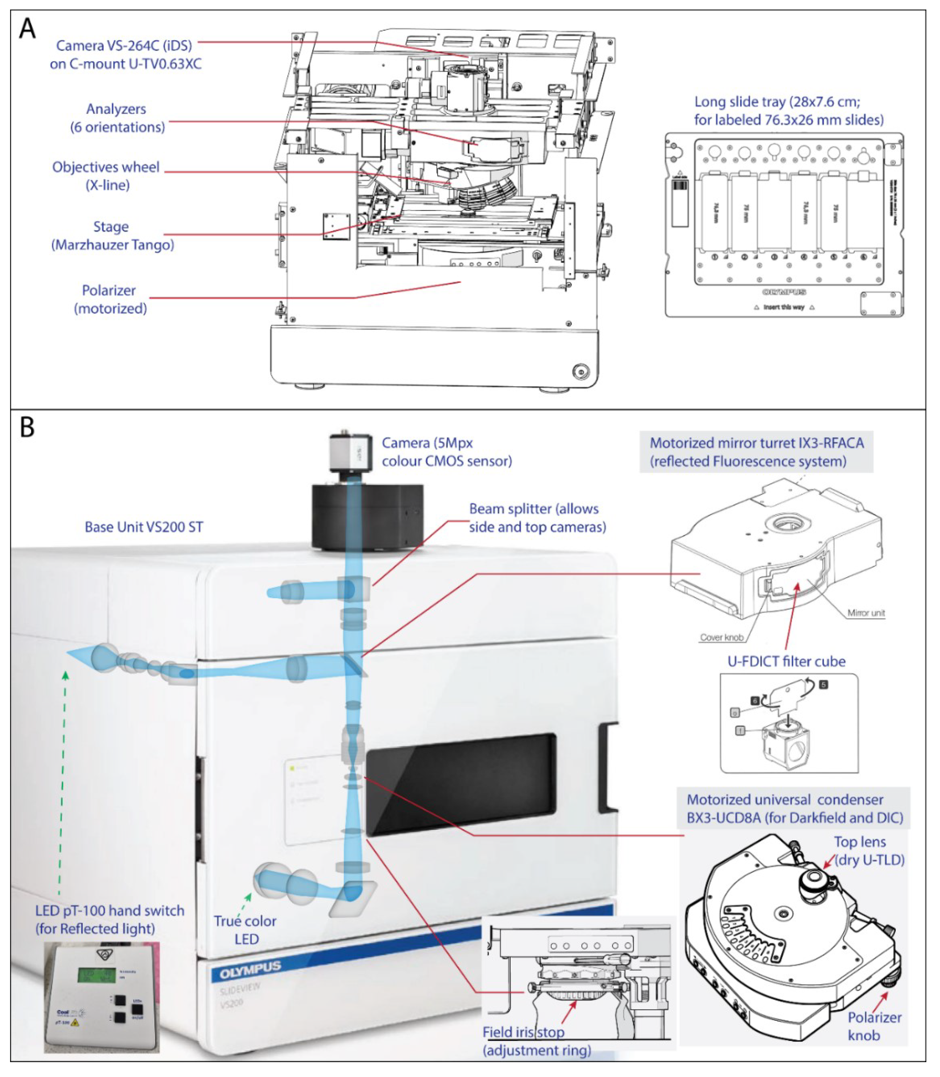
2.1.1. VS200 Slide Scanner

The instrument used here is the VS200 single tray (ST), a first-generation integrated optical microscope designed for research (not diagnostic) purposes. Its original setup can perform brightfield (BF), fluorescence (FL), and phase-contrast (PH) microscopy and their combinations. FL uses specialised techniques, such as confocal microscopy, to study cells in z-stacks, dark-field (DF) for following stem cell colonies within referential overviews, and differential interference contrast (DIC) to better understand optical path-difference ‘relief’, all of which require special filters. In collaboration with the manufacturer Evident Scientific (formerly Olympus), we have repurposed the VS200 polarised transmitted (POL), and brightfield reflected light (RL) modalities to perform petrographic plane-polarised (PPL) and cross-polarised (XPL) observation in multi-angle polariser orientations. An overview of VS200 is shown in Figure 1, and a more detailed explanation is given in Supplementary Materials S1 (VS200 calibration).
Notwithstanding the advances in geological WSI, there is also growing interest in studying non-geological materials in PPL, XPL, and RL, for instance, to characterize the human brain connectome [19], small organisms [20], parasites [21], and viral cytopathic effects [22], providing contextual analysis of molecular bond or fine structural form in cells. For example, the VS200 PPL RL has already found applications for human cartilage observations in collagen networks without staining and XPL for counting growth rings within fish otoliths (listed as an application note on the Evident webpage).
The base unit VS200 ST works with a single sample tray in which slides are automatically detected with inventory and proximity sensors. We used 6-pocket trays for either long (75 mm) or short (50 mm) thin sections. The former is a standard size for biological slides, while the latter tray is an adaption achieved with a tray insert for the 50 mm slides most widely used in earth sciences (Figure 2). Following a tray exchange, filled pockets are detected with the ‘2×’ objective lens and optional label QR codes are read. Usually, slides are scanned in two steps, first with an overview image (2×) followed by a detailed higher resolution scan. The workflow settings can be saved for each modality in ‘scan projects’ that will show up to other users (‘scan’ tab interface). Both steps include the calculation of auto-focus and auto-exposure within the defined scan area based on a grid of measuring sites over the detected sample area.
Vertical focus is found by moving the nosepiece turret as the stage only moves in the x and y directions to preserve the entering position of the automatic front door of the instrument. The advertised z-accuracy of the Marzhauzer stage is +/− 100 nm, enabling high-quality acquisition at any magnification. The focusing algorithm might not find a suitable starting focusing distance if a glass slide is off range, for example, being of considerably different thickness than the typical slides, or the thickness violates the security distance to prevent the collision of the sample and objective front lenses. Effective and unsupervised scanning thus requires the use of consistently dimensioned thin sections, but z-stage recalibration can be performed to allow scanning slim mounts (and loose materials) attached to glass slides. The sample focusing distances can be measured in a ‘single’ scan with ‘semi-automatic’ focus mode and, assuming perfect horizontality (the stage is adequately manufactured) and sample flatness (+/− 5 µm), it can serve as a digital calliper.

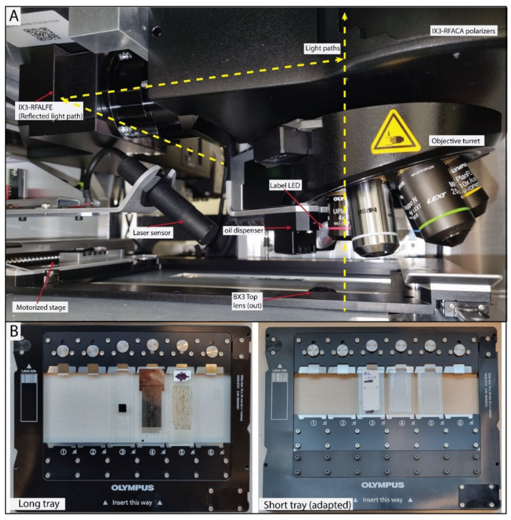
2.1.2. Repurposing the Scanner for Polarised Light Microscopy

The main changes made to the standard VS200 were necessary to perform TL-PPL and XPL observations with low (2×, 4×) and medium (10×, 20×, 40×) objective magnifications at different polarisation angles. The standard ability of the instrument to combine FL/PH and FL/DF was disabled in favour of BF/POL. The motorised polariser PPL-0 was oriented E-W, and the wheel analyser (XPL-0) was calculated to be N-S, relative to the imaging coordinate system that is perpendicular to the tray insertion direction. In addition, a BF RL path was added and turned into a mandatory modality that allows focusing on the sample surface at any magnification, which is not easily attainable in transmitted light (TL) due to the sample thickness (30–35 µm) exceeding the depth-of-field.
The transmitted (BF design) and reflected (FL design) light sources are true-colour LEDs located at the bottom and side of the base unit, respectively (Figure 1). Most light path components are motorised and can be controlled from software for single or batch scanning, with full setting freedom in the ‘manual acquisition’ panel. The software was informed about the physical modifications to the microscope to avoid in-built alerts (‘home’ menu). The RL setup is developmental and uses an analogue hand switch (pT-100) for turning on the LED source and a manually adjustable shutter within IX3-RFALFE (Figure 2) that have not yet been integrated into ASW software.
The dry objectives installed in the nosepiece are listed below in order of increasing magnifying power along with some of their properties:
  • PLN 2X. Achromat: 2.691 µm/px. Working distance (WD) = 5.8 mm UIS 2 NA = 0.06.
  • UPLFLN4X. Semi-apochromat: 1.369 µm/px. WD = 17 mm; OFN26 NA = 0.13.
  • MPLFLN10X. Semi-apochromat for no glass cover slip: 0.547 µm/px. WD = 11 mm; OFN26 NA = 0.30.
  • MPLAPON20XLEXT. Plan apochromat for no glass cover slip: 0.273 µm/px. WD = 1 mm FN18 NA = 0.6.
  • MPLFLN40X. Semi-apochromat for no glass cover slip: 0.137 µm/px. WD = 0.63 mm; CFN26 NA = 0.75.
All the chosen objectives have spherical aberration for more than 2 colours, except PLN 2×. The no glass cover slip objective designs assume a point source at the rock surface. The MPLAPON objective series can be dedicated to simple polarised observation incorporating field curvature correction. The MPLFLN series has limitations in polarised light observation. Furthermore, RL is not working with the 2× objective due to self-reflection on sample surfaces and, on the short pocket tray, yields imperfect shading calibration at 20× and 40×, despite successful Kohler illumination due to slight tilting of the prototype short-section tray. In all cases, the nominal LED lamp voltage used to achieve sufficient illumination was low (around 35–40% voltage), with the BX3 aperture stop opening at 75%.
At the top of the optical light path sits the IX3-RFACA turret, normally hosting 6 dichroic mirrors and excitation filters that were replaced with wire grid polarisers (analysers). They were positioned manually at nominal 18° incremental steps from the polariser (+clockwise rotation, 1° steps precision). The corresponding extinction positions of the fully rotatable polariser were saved in the software for all 6 analysers. For setting the positions, we recommend using a master rock thin-section with large isotropic minerals (in our case, a biotite-garnet gneiss) at practical and constant camera exposure levels (see Table 1). The fine extinction position is found with the help of the digital histogram adjustment feature in the ‘live’ view mode. Checking the lower tail in the histograms and observing the fringes of the sample allows finding full XPL extinction positions. The current six-analyser turret will eventually be replaced by one motorised analyser for accurate and systematic azimuthal crystal orientation estimations (2D only).
The bottom of the light path uses a motorised condenser (BX3-UCD8A) that has a dry top lens and enables working with the depth-of-field of higher magnification objectives (10×, 20×, and 40×), producing smoother images that are much more informative than 2× and 4× (see, e.g., Figure 3). Therefore, transmitted light skips most optical elements (phase contrast rings and DIC prisms) that are not required within a petrographic microscope and instead uses the single motorised polariser.

2.1.3. Olympus ASW Software

The microscope application software (ASW v3.3) is flexible for operating and calibrating the instrument and allows tailoring petrographic acquisition routines for multi-paged files of slide surfaces (giga-pixel) and z-series volumes (multi giga-pixel). The developed routines trick the system into obtaining multi-band nominal fluorescence acquisitions, which, given that the original filters were replaced with polarisers in the IX3 turret are multi-pol WSIs. All image modalities are acquired in a single-round batch acquisition in ‘fluorescence’ mode by making up a list of scanning modalities in a ‘scan project’ without losing individual white balance. The first ‘channel’ in the list is used for focusing and stitching the entire list.
The controlling PC is an HP Z2 Tower G4 workstation (i7 9700K @3.6 GHz 8 threads, 32 GB DDR4 RAM 1330 MHz dual channel) with a primary (PCIe Gen3 NVMe SSD of 1 TB, Samsung, Suwon, Republic of Korea) and a secondary (SATA 600–7200 RPM HDD of 2 TB, Seagate, Cupertino, CA, USA) disk. The primary disk is partitioned between a main Windows 10 installation (700 GB) and the VS200 swap memory (255 GB), reaching read and write speeds of 3400 and 2400 MB/s (measured with CrystalDiskMark v8.0.4). The secondary disk saves the slide scanner dataset with read and write speeds of 180 and 164 MB/s. Scanning has been successfully tested in all magnifications, but RAM memory issues occur at 40× and sometimes at 20×.
The ASW software produces files containing the Images of each slide in multiple planes (or pages) of information after the last round of a batch scan. These are in a coordinate space that is defined by the preconfigured slide shape factor (short slide, long slide, with or without labels) and applies to all user-defined scan areas within a slide. The WSI files are in a paired folder structure containing sub-folders with images recurrently downscaled and resampled (image pyramid) and a header containing all the experiment metadata (cellSens format: *.vsi). The header (normally up to 10 MB) can read the folders and contains all the experimental metadata required for further enquiries and navigation within 10× image pyramids of unlimited size (~13.5 GB, given that *.vsi allows JPEG compression). The compression seems not to affect the image processing quality when translating as *.tif (see Supplementary Materials S1 (Image analysis pipeline)).
Optionally, the user can manually build an apparent z-stack in which multi-pol navigation is intuitive, allowing viewers to zoom into areas and seamlessly change viewing modality (18° rotation and switching between RL, PPL, and XPL) simply by rotating the mouse wheel. This is only recommended for WSI at 4× *.vsi data trees (due to time and memory constraints).
In terms of acquisition time, it takes ~24 min to obtain a series of 14 WSI images (2 RL, 6 PPL, and 6 XPL) with the 10× objective lens. This time includes a label (QR-code) and overview scan (thumbnail), and simultaneous stitching and uploading to the local server (1 file at 140 Mbps; 2 files at 240 Mbps). The acquisition product is a single file in which each image has 3 layers (RGB) containing approximately 790 frames (tiles of 2456 × 2054) with ~20% overlap and a blending area of 8 pixels (Gaussian alpha). Tiles are acquired in a meandering path (within sub-areas) tied to the focus map reference frames. The output data tree scans are around 75 × 44 K pixels constituting a total of 10.3 K image tiles. The dimensionality of a single orientation image is: X, Y, Channels = 3, Z levels = 1, Time points = 1, containing ~700 stitched and blended original tiles.
Further acquisition customisation is via the configuration of the ‘expert’ mode (activated via press-hold shift + left click), enabling the settings tab, with the option to store the image tiles in a separate folder of the workstation. Moreover, the user can change the scan logic from ‘switch channel before moving XY’ to the opposite, at the expense of increasing the mechanical wearing of the motorised parts. This eliminates the multi-modal stage drift and dramatically increases the acquisition time. The XY movement is performed in meandric sub-samples that can have a specific focus map, risking a blurred sample trail if the algorithm does not find a focus distance (inadequate illumination, thin section of different makeup, etc.). To avoid partially unfocused trails in 20× and 40×, it is recommended to perform a focus map in ‘extra high’ site density, especially on tilted slides or thin sections exposing minerals of very different hardness (i.e., topography from polishing). Furthermore, inside the ‘scan’ panel, the areas can be imaged with z-series stacks that will automatically set up the scans at increasing focus map depths for producing virtual-Z (and EFI) images. This is a technology inherited from confocal microscopy designs.
For learning, teaching, and collaboration, the files are not downloaded onto the online PC hard drives but saved on a local server and visited using the OlyVIA freeware v3.3. Note that the connection to our local server is broadband and much faster than the usual bandwidth to a regular local area network (LAN). An example of a typical image data tree obtained on a spinel-harzburgite (olivine, orthopyroxene, clinopyroxene, spinel, and alteration products) is shown in Figure 4. OlyVIA software allows users to navigate and zoom on the sample image and review histograms and experiment metadata. In the server’s backend, the infrastructure with integrated security settings (Net Image Server SQL, NIS-SQL) works satisfactorily to the small-scale needs of the academic department, though within the institutional proxy server connections and internet logon (remote VPN).

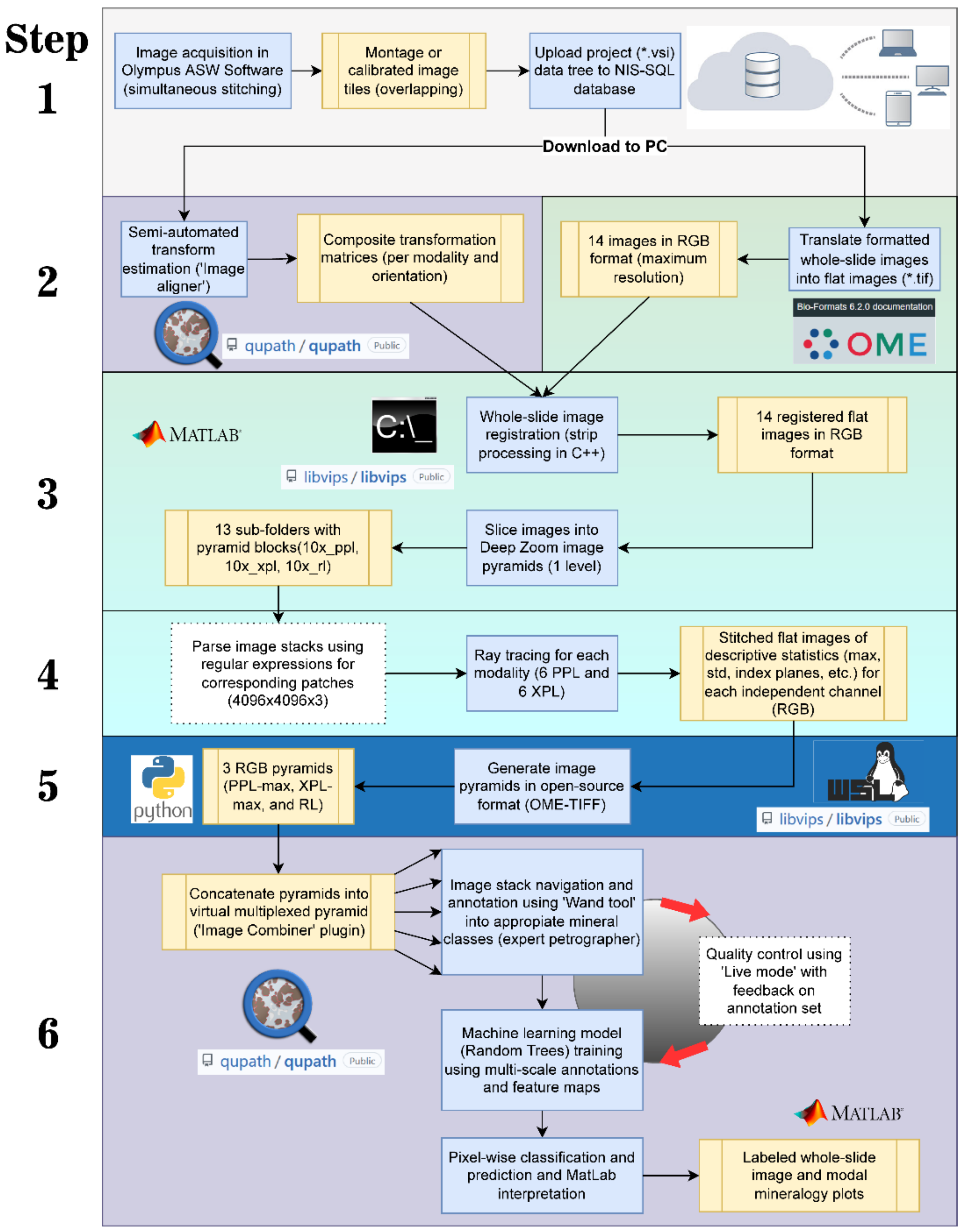
2.2. Image Analysis Pipeline

The VS200 is an effective tool for surveying large thin-section archives at low magnification, from which interesting rock specimens for higher magnification scanning are identified. High-resolution WSI and sophisticated image analysis are intended for specimens of high research value, typically also requiring chemical microanalysis. For this pilot project, we scanned a total of 8 thin sections, many with significant legacy data, including SEM-EDX phase map modal mineralogy [23,24]. For trialling the software pipeline, lithologies were selected to cover from peridotites to mafic granulites to granitoids, including contrasting grain sizes.

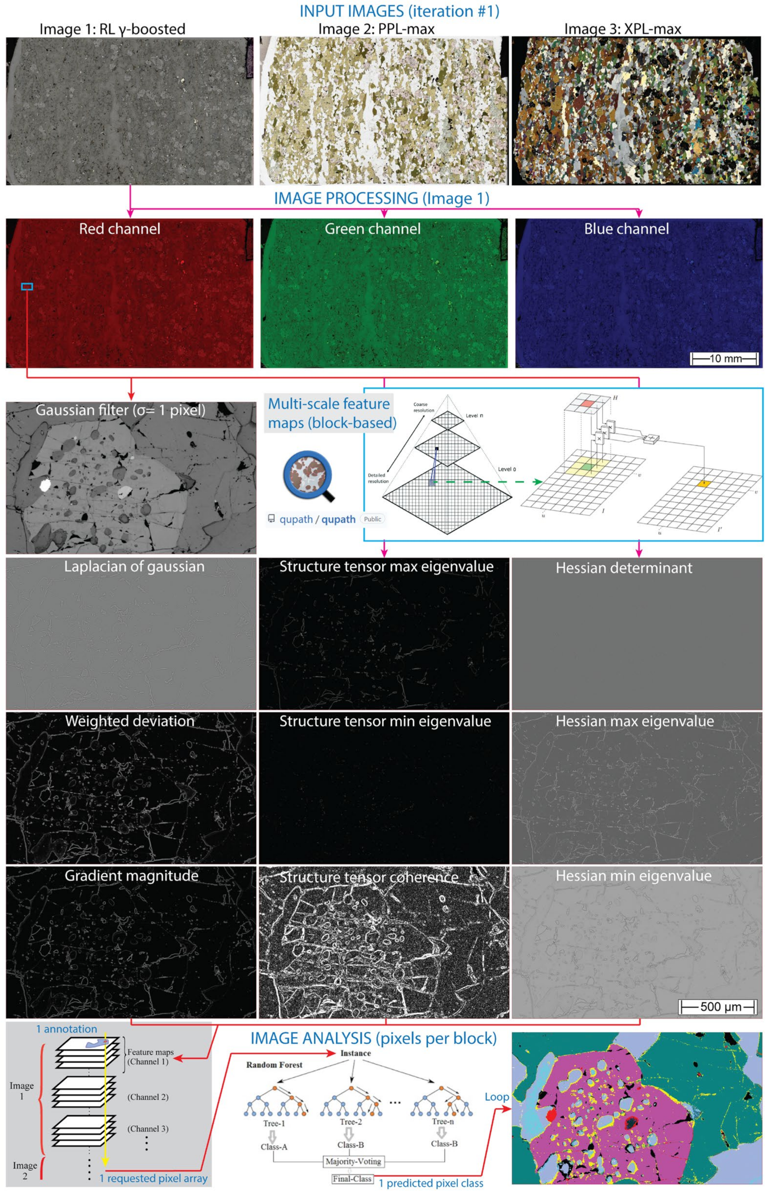
2.2.1. Image Analysis Pipeline Summary

A prototype image analysis pipeline was developed by forking open-source software. It enables saving intermediate image products that permit iterative improvements and assessing reproducibility. Under constant supervision, the semi-automated 6-step pipeline can process one thin section at 10× in 3–5 h (using CPU parallel threads in an Alienware X15 R1 computer). The details of the software pipeline and its two variants (Option A and B, see flowchart in Figure 5) are given in Supplementary Materials S1 (VS200 calibration). Option A requires more user input, while Option B is its pythonic evolution automating steps 2 to 5 but with more stringent ‘perfect’ image input requirements.
The first step is image acquisition, for which thin sections are set up in the tray, followed by batch scanning with our recommended settings. The resulting files are uploaded to the server allowing multiple users to pinpoint interesting samples and ROIs. On interesting samples, higher resolution scans are downloaded from the server before progressing to step 2.
In the second step, the software QuPath and a customised MatLab script (see GitHub page) are used to independently estimate the geometric transform matrices registering each WSI modality in best-found co-registration with the fixed image (RL). This step is performed manually for one scan in each modality and then semi-automatically with translations for every corresponding multi-pol plane. Follow-up exportation uses an image pyramid translator that understands any format (not only *.vsi).
In the third step, the pyvips library is deployed for applying the transforms (rewritten for the MatLab script) and registering the flat images. This library was chosen due to superior computational efficiency (C++ language). All operations are orchestrated from the script that interprets the file names (‘parsing’) to understand which images belong to which folder and to produce a sub-folder structure for subsequent steps. Because there is no RAM limit in using pyramid blocks, the minimum feasible size of the blocks needs to be judged against the user PC capabilities for adequate data management and transfer rates (MB/s).
In the fourth step, the sub-folders (for PPL and XPL) are taken over by a MatLab script for descriptive statistics and dimensionality reduction (reducing the six multi-pol images to one). The choice of the equations processing each pixel or the modalities participating in the image stack calculations is flexible. With pixel classification in mind, the user chooses the most adequate representations (explained in detail in the results section). The implementation was kept simple to enable using parallel threads but vectorisation to lessen operation time. Later, the new blocks are stitched either in MatLab or Python to produce a collection of ray-tracing flat images (PPL-max, XPL-max, and RL).
In the fifth step, pyvips converts the three images into OME-TIFF image pyramids for computationally cheaper navigation and operation with the datasets by specialised software. Optionally, the ray tracing (or any) flat images can be imported to ASW for generating z-stacks for (web-based) OlyVIA viewing.
The final image analysis is performed in QuPath (described in the following subsection). The ‘Image Combiner’ is deployed for combining the images into one multiplexed image pyramid that can be navigated, annotated (wand tool), and viewed using convenient colouring settings or screen views. Then, the ‘Pixel Classifier’ is used for performing machine learning semantic segmentation from internal training pixel data of image annotation areas according to the listed ‘feature’ maps. No new images are saved as all user inputs (and modifications) live only within the QuPath project as a GeoJSON file (Megabyte file). Later, the phase maps are re-interpreted in a MatLab script.

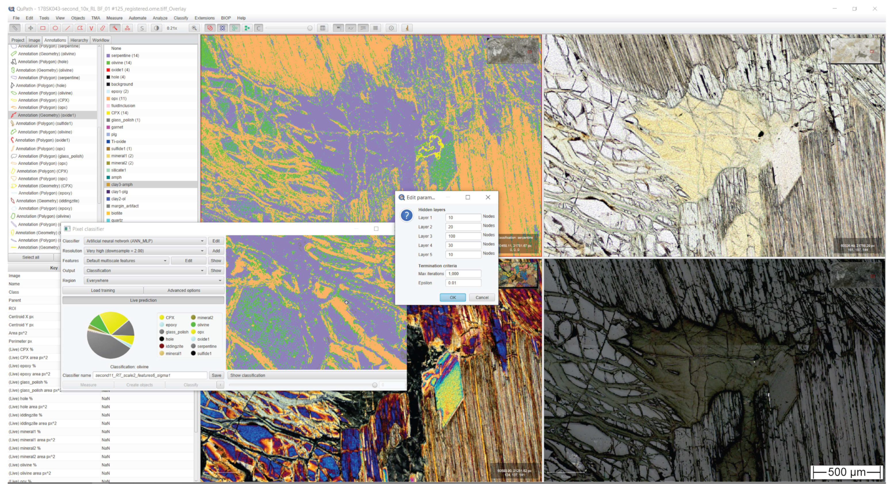
2.2.2. QuPath Software

QuPath [25] version 0.3.2 is a cross-platform open-source software for digital histopathology that can work offline on an average researcher PC using image pyramid formats. The software was developed for cell morphological analysis and positive (cancerous) cell detection with the ‘Object Classifier’, and it was not until the significant improvement of the ‘Pixel Classifier’ around version 0.2.0-m5 that working with any type of imaging data became easier. It performs semantic segmentation that separates and visualizes class masks (not grain instances) at a selected resolution level in the software canvas.
In normal use, the software handles multi-gigapixel WSI (single <30 GB) in 2D brightfield microscopy at very-high magnifications, typically scanning sectioned tissue pucks. However, multiplexed analysis is possible as QuPath was designed to also analyse confocal fluorescence microscope WSI. In this use, an efficient and feasible computational balance needs to be kept between the number of channels and the whole-slide image extension (at constant ‘cube’ volume), where dimensionality reduction and ray tracing are good options to maximise the information input. Pixel classification can temporarily freeze the computer for a few seconds when ‘live’ mode is activated during training, but control resumes. Previous workers [26] have trialled the console scripting in sedimentary rocks. The software documentation explains the full image analysis process [27].
The software incorporates extensive annotation (Figure 6) and visualisation tools (Figure 7). The canvas can be updated by modifying the z-stack/t-series plane index with a slider, transparency, and colour channel contrast of the opened images. Annotations and detected objects can represent and display relationships (hierarchical object-based data model) between very large numbers of GeoJSON objects in an efficient and intuitive manner across scans. Internally, the OpenCV libraries work together to support fast and interactive training of machine learning algorithms (Random Trees and Artificial Neural Networks). Analysing each pixel, the internal functionalities access an ‘image server’ that performs pixel requests from any pyramid level. The platform loads, caches, and processes FoV data block-by-block as the user interacts with the software front-end; thus, waiting for full image loading is not required.
Of particular use in petrography is the possibility of annotating imaging modalities separately. This allows the identification of features (e.g., reflective minerals) in one image modality, even though they may not be identifiable in the other two (PPL and XPL). This is performed in the channel selector sub-menu (shown on the right-hand side of Figure 6). Using the ’wand’ tool (region-growing algorithm), images are annotated until an extensive area of the section has been covered (including artefacts). It is recommended to find the largest class diversity and meaningful feature maps for training.
The ’Pixel Classifier’s closest relative in the Fiji ecosystem is the Trainable WEKA Segmentation (https://imagej.net/plugins/tws/ (accessed on 16 January 2023)), but QuPath is designed for WSI. The number of directly supported ImageJ [28] plugin functionalities is increasing with the user base. Essentially, the image filtering operations are performed on each channel (Figure 8) and are oriented to highlight ‘blobby’, ‘stringy’, and ‘patchy’ textured areas (https://qupath.readthedocs.io/en/0.4/docs/tutorials/pixel_classification.html (accessed on 16 January 2023)). Filters such as the Gaussian (smoothing) and gradient magnitude (edges) are available that yield reliable generalisations to broader image models. These turned out to be mandatory options for using QuPath for optical mineralogy purposes.

3. Results

The results are presented in four subsections beginning with a brief assessment of the preferred scanner setup. Next, we describe optical ray tracing on thin sections of various mineralogy and then present the results of petrographic observations with ray tracing images. Finally, we present phase maps and modal mineralogy estimates from image segmentation.

3.1. Findings from Instrument Calibration

The custom optical illumination calibrations (exposure, white balance, shading) for our application were developed over a trialling period with the finally selected tools listed in Table 1. Improving workflows and imaging outputs and ASW workflow development using the same wizard menu as when a new VS200 was first installed. Both BF and PPL are easy to calibrate using the VS200 calibrating slide and under normal operating conditions. It is found that compared to a camera-equipped traditional microscope, the instrument presents superior calibration steadiness with reduced servicing time. For instance, the LED lamp behaves similarly to a halogen lamp, having a long life duration and even luminosity. The user can edit the hardware, optical components, and illumination calibrations, making them specific to each modality (PPL, XPL, and BF RL) and magnification combinations. Further details on the calibration are given in the Supplementary Materials.
The polariser orientation is the most important setup. It requires inserting a master thin section for which we selected a gneiss with biotite and garnet. Biotite is used to test the orientations of the polariser and analyser since, in PPL, it should turn dark brown when oriented E-W (//polariser) and pale light yellow when N-S (//analyser). Garnet was used to find the optimal extinction with the help of the default digital histogram.
The sample contains plagioclase that was useful to set the white balance (WB). The camera WB is generalised for the multiple polarisation orientation angles of the same modality. It consists of reproducing natural light (true) colours and acquiring each RGB channel with the same distribution when viewing the histograms over grey areas. The ASW software interface in ‘manual control’ allows clicking an ‘illuminant’ value (true grey pixel or ROI) in ‘live mode’ (e.g., quartz or plagioclase crystals) for balancing by applying multiplying RGB factors to the raw images and can be found in the camera settings.
An important aspect of scanning rock thin sections is camera exposure. Rather than selecting automatic exposure, one manual exposure setting across a suite of multi-pol acquisitions is strongly preferred to avoid intensity variations between multi-pol scans. Auto-exposure, determined by the software on a handful of frames ahead of batch scans, can lead to sub-optimal exposure settings, particularly in heterogeneous samples, rocks containing minerals with strong crystallographic orientation (fabric) and generally coarse-grained assemblage (e.g., peridotites). Instead, manual exposure settings using an optimal dynamic range are defined in ‘live mode’, ensuring that there are no overexposed (highlighted in red) and underexposed (blue) pixels. Exposure times are preconfigured using manual exposure levels for all observation methods, but generalised settings are readily found for the most common rock types.
The next principal calibration is shading. It consists of a (residual) intensity gradient towards preferential tile directions, such as corners and overlapping areas. It is advised to iteratively perform WB before and after shading correction in the case of unnatural patterns arising from the underlining shading model. The XPL shading correction used two thin sections of large quartz crystals in contiguous pockets. It is important to carefully place the FoV (at each magnification) over pristine areas of the mineral at constant normal operating exposure times. When one of the crystals is near extinction, the other crystal produces better results (due to single orientation). This process removed all but the very slightest shading observed in grey crystals on overlapping areas. This might be related to the optical path (no coverslip samples and objectives not dedicated to polarisation). For RL shading calibration, we opted to use a mirror-quality silicon semi-conductor wafer. It yields optimal and pristine reflection on the entire FoV.

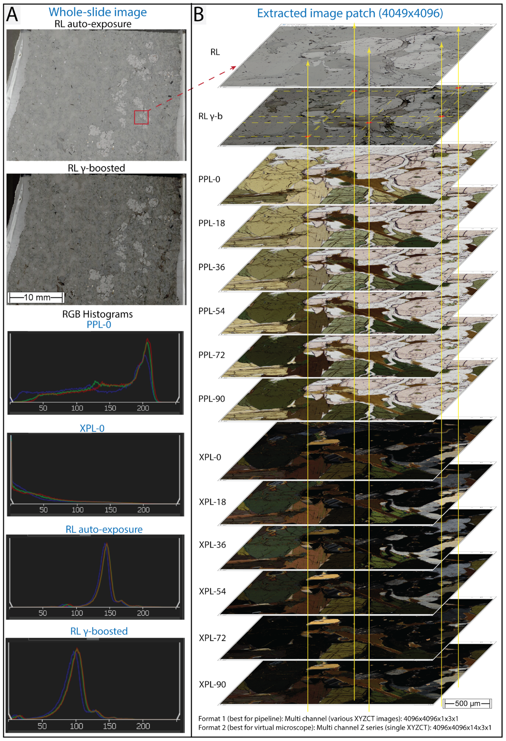
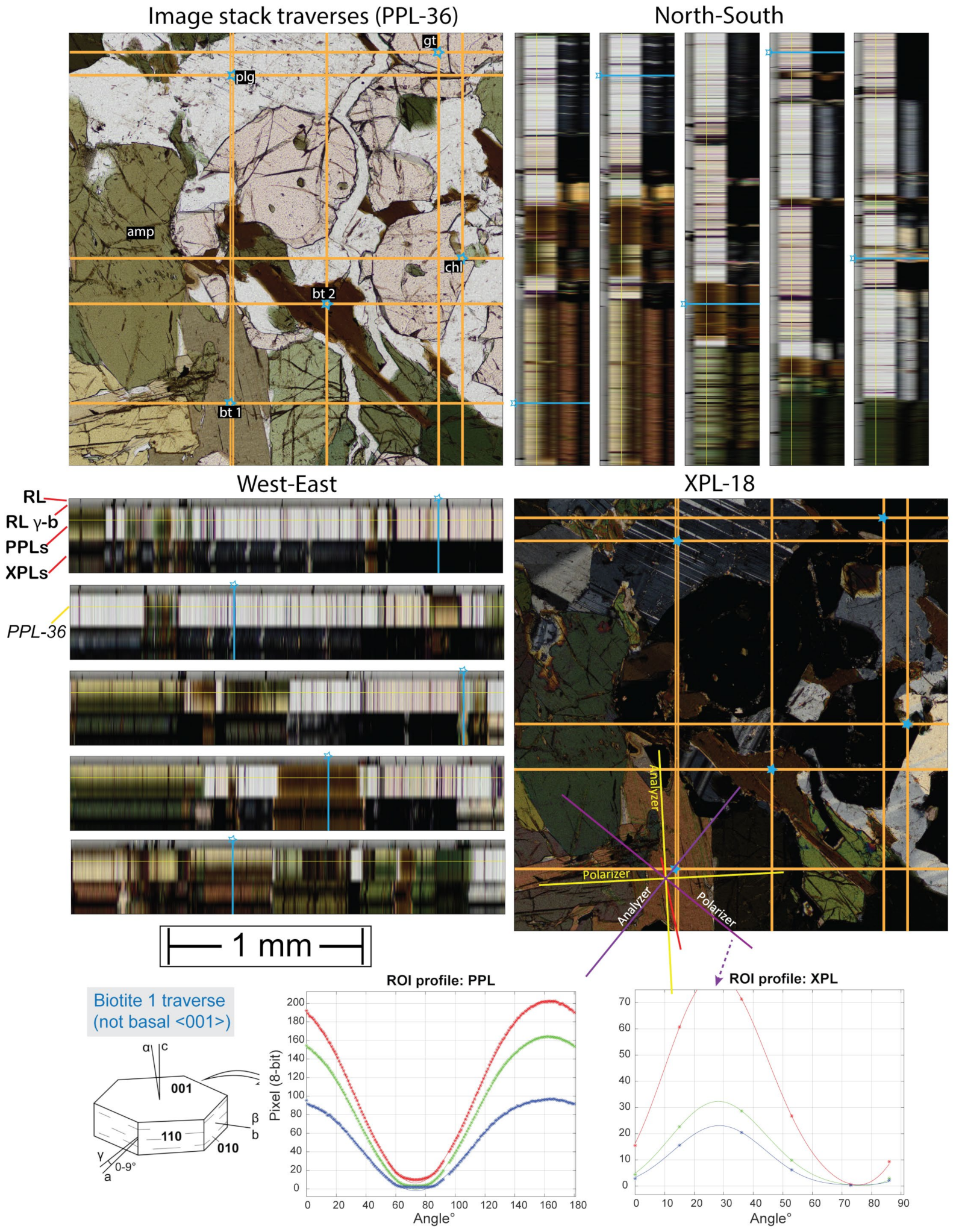
3.2. Optical Ray Tracing

Ray tracing serves three main purposes for digital optical mineralogy: (i) it reduces pleochroism in PPL; (ii) it avoids extinction in XPL [17,29,30,31,32,33]; and (iii) it reduces the number of image modalities having to be handled by the software in which pixel classification is performed.
In the simplest terms, the six multi-pol PPL and XPL stacks are each reduced into one new ‘composite’ ray trace image. Figure 9 shows an example of a perfectly registered whole-slide image pyramidal stack and an extracted region with five rays that are traced through RL and multi-pol PPL or XPL images. Different minerals show contrasting colour variations depending on their crystallographic system and orientation within the sample volume, where grain contacts might show mixed behaviour.
Statistical analysis is performed on the R, G, and B channel values of all six pixels from the PPL (or XPL) multi-pol stacks corresponding to the same location on the thin section. A new pixel is then generated containing the descriptive statistics (‘mean’, ‘max’, ‘min’, ‘sum’, ‘std’, ‘median’, ‘incremental PCA’), and the collective pixels of the entire scan are combined to create the new image. The statistical analysis is performed in a processing loop for every image pyramid block (registered images). The computation uses multi-thread CPU processing in MatLab software with an image patch size of 4096 × 4096 so that it can fit in the RAM memory. At 10×, ~200 patches are processed in 6 min 40 sec for the simplest functions ‘max’, ‘min’, and ‘mean’, in 8 min for standard deviation (‘std’), and in ~23 min for the more-complex incremental PCA that requires the data twice. Offline montaging and pyramiding of the images were then carried out at the end of the Python workflow (Option B).
Figure 10 illustrates a static overview of orthogonal traverses (orange lines) of the five ray traces relative to the grain mineralogy of the image patch stack. Within Fiji, this can be visualised dynamically. Each vertical traverse represents one pixel width. and the colour gradient (sinusoidal wave) within each traverse transitions from RL, γ-boosted RL, six-angle PPL, and six-angle XPL from left to right. For example, the fourth traverse shows an intersection with garnet marked with a blue line. Here it is evident that the colour in PPL does not change, and in XPL, the garnet remains black. In the horizontal traverses, the colour bar reflects, from top to bottom, RL, γ-boosted RF, six-angle PPL, and six-angle XPL. The second-lowest and lowest traverses show intersections with two differently oriented biotite grains showing a different PPL colour at each rotational angle. In each traverse, for most pixels, the colour information largely reflects the mineralogy, but the multiple dark bands across PPL angles show textural patterns, such as grain boundaries, inclusions, fractures, and cleavage, and XPL shows polysynthetic twinning and pinpoints chlorite crystal locations having high interference colours, which helps distinguishing quartz (yellowish at certain orientations) from plagioclase (grey).
For each pixel, RGB values can be extracted and plotted versus the polariser angle (two examples are shown at the bottom of Figure 10). The resulting plots show a clear 90° spectral period for XPL, while PPL can be fitted with a 180° period fixed-boundary condition. Furthermore, from the orientation of the maximum interference colour of the spectral fit line (purple arrow), it is possible to work out the true orientation of the polariser–analyser pair (yellow lines) and their relative orientation (purple lines) when biotite #1 (parallel extinction) cleavage (red line) is at maximum interference colour.

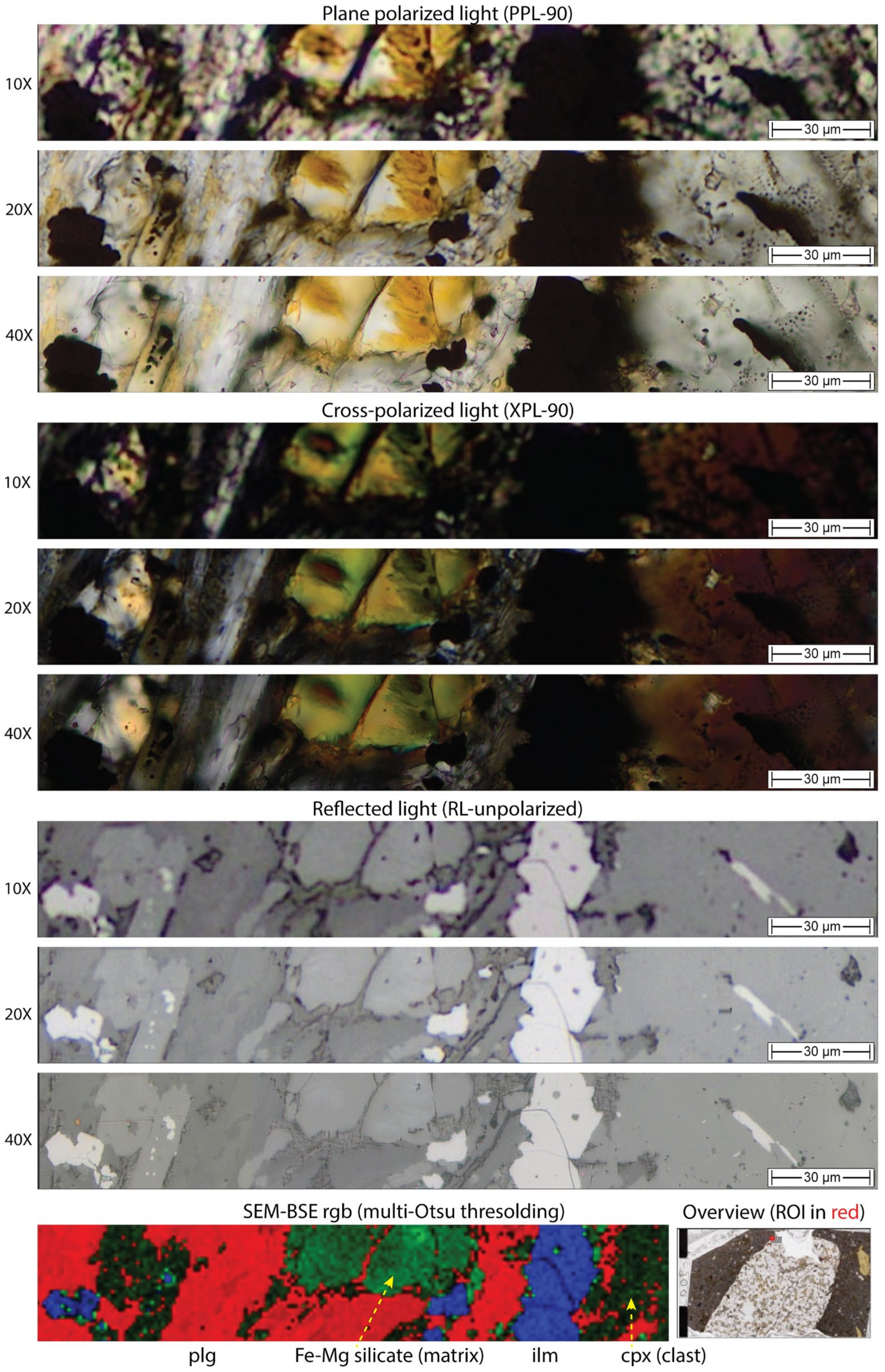
3.3. Petrographic Observations on Ray Trace Images

Figure 11 shows a variety of statistical ray tracing images for three samples of very different mineralogy: coarse-grained spinel-harzburgite 17-BSK-43; hornblende granulite 6KB-67; and granodiorite 2512-PTS. For all three diverse rock types, it is found that PPL-max and PPL-min greatly reduce the effects of pleochroism in PPL. This is most clearly seen in the hornblende of the granulite, which in PPL-max shows limited hues of green and in PPL-min ranges from dark green to brown-green. In both statistical representations, the pleochroism is thus much reduced compared to the colour variation shown in any given PPL, where hornblende ranges from pale yellow-green to dark green (e.g., Figure 10). Similarly, the pleochroism of biotite in the granulite and the granodiorite is much reduced, consistently showing yellow to pale brown colour in PPL-max and dark brown in PPL-min. In the granodiorite, PPL-max also easily identifies altered biotite (largely green chlorite).
It was found that PPL-max affords the clearest distinction of phases. The reduction in pleochroism for orthopyroxene in the harzburgite is less pronounced both in PPL-max and -min. This is, in part, due to the colouration (bronzite) of the orthopyroxene reflecting crystallographically oriented clinopyroxene exsolution lamellae. In addition, the strongly different intensities for differently oriented orthopyroxene crystals (parallel extinction) remain, in part, because the six angles at which the PPL scans were obtained only cover half the periodicity of pleochroism (90 instead of 180°) as also seen in Figure 10. Additionally, the bluish tint in PPL-min exists because this section was made on a 0.3 mm thinner quartz glass slide, for which the standard instrument calibration resulted in inaccurate WB. This can be seen in the mismatching RGB spectra for PPL-0 in the histogram in Figure 4.
Information is also contained in the standard deviation (PPL-std) images, where pleochroic minerals have stronger intensities than colourless minerals or phases of a single isotropic colour. As a result, garnet in the granulite appears nearly black, similar to plagioclase. In the felsic granodiorite, the PPL-std image is very dark because of the non-existent pleochroism (and hence low standard deviation) of quartz and the feldspars. In the harzburgite, orthopyroxene has stronger intensities in PPL-std than olivine and serpentine (veinlets). The harzburgite PPL-std image shows noisy artefact stripes of image tiles in brighter colours that are horizontally appearing at regular distances. This is caused by slight stack misalignment, increasing the standard deviation of each pixel and image stitching artefacts due to x-y stage drift.
In cross-polarised light, it is evident that XPL-max shows the maximum interference colour of the assemblage. In harzburgite, nearly all minerals show vivid colour with only one orthopyroxene oriented close to perpendicular to the c-axis (near extinction regardless of multi-pol angle). The XPL-max image also strongly exposes serpentine, which due to its cryptocrystalline nature, remains dark, but in low-angle cracks, it becomes brighter due to the over- and underlying wedges. At high zoom levels, XPL-max also shows clinopyroxene rimming orthopyroxene, but it is harder to distinguish from olivine due to colour overlaps. In the granulite, XPL-max helps to distinguish between amphibole and biotite while also exposing the generally banded fabric with garnets in extinction and plagioclases showing well-defined grain contacts.
The XPL-min images show some grains that are not in full extinction (i.e., black) because only six multi-pol angles were used at 18° spacing, missing full extinction. Furthermore, in those instances, the faint colours in XPL-min are quite similar to XPL-max, demonstrating that for a given crystal orientation, interference colour (retardation) is independent of the effect of the relative orientation between the optic indicatrix and polarising pair. The plagioclase grains’ internal features (zonation) and distinction from quartz (yellowish grains) are better observed in XPL-min than XPL-max. In the granodiorite (2512-PTS), distinguishing plagioclase, quartz (yellowish in XPL-min), and microcline is challenging based on XPL colour alone due to grey tone overlapping, but XPL-max reveals muscovite locations, which are not readily seen in PPL. Although microcline presents the characteristic grating structure twinning, its anhedral shape in this rock makes it difficult to discriminate from subhedral and equant plagioclase or the unaltered quartz (yellowish in XPL-min). Notably, grains finer than the thickness of the section (~35 µm) or very low-angle contacts might never go into extinction since there is no single orientation that would darken all stacked grains, and their mutual intergrowths might scatter light. This exposes clay-filled micro-fractures (Figure 12), which are not easily seen in PPL. The XPL-min image also picks out tiny mineral inclusions within fractured grains. The granodiorite contains several accessory minerals, such as titanite, prismatic apatite, and zircon, whose optical appearance will be discussed in the next sections.
The appearance of XPL-std in many ways resembles that of XPL-max. It has two advantages. First, because it combines data from six pixels rather than extracting a single-pixel RGB value, the resulting image is smoother than XPL-max. Secondly, compared to XPL-max, -std decreases the channel intensity range by a factor of 2   .
In summary, the most straightforward reduction in dimensionality is obtained when the six multi-pol PPL and XPL images are each projected into the ‘max’ values, and these were subsequently used for image segmentation. However, other statistical operations can contain an additional value, for example, in identifying the least-altered feldspar around alteration veinlets (XPL-min). This could readily be used to inform the selection of spot analyses, e.g., for Pb-isotopes by laser-ablation ICP-MS, where pristine feldspar is needed to avoid labile Pb.

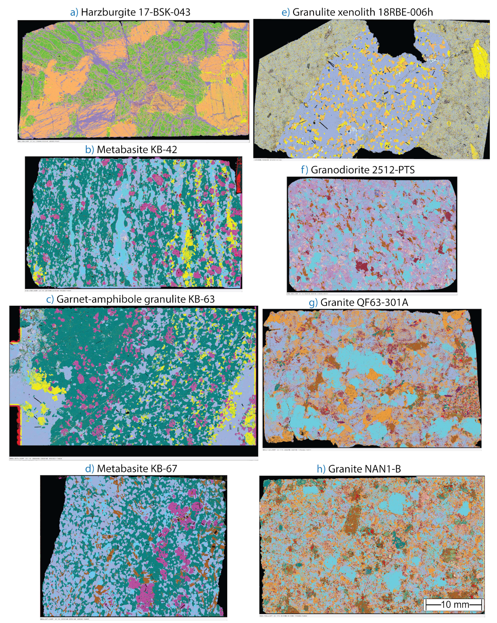
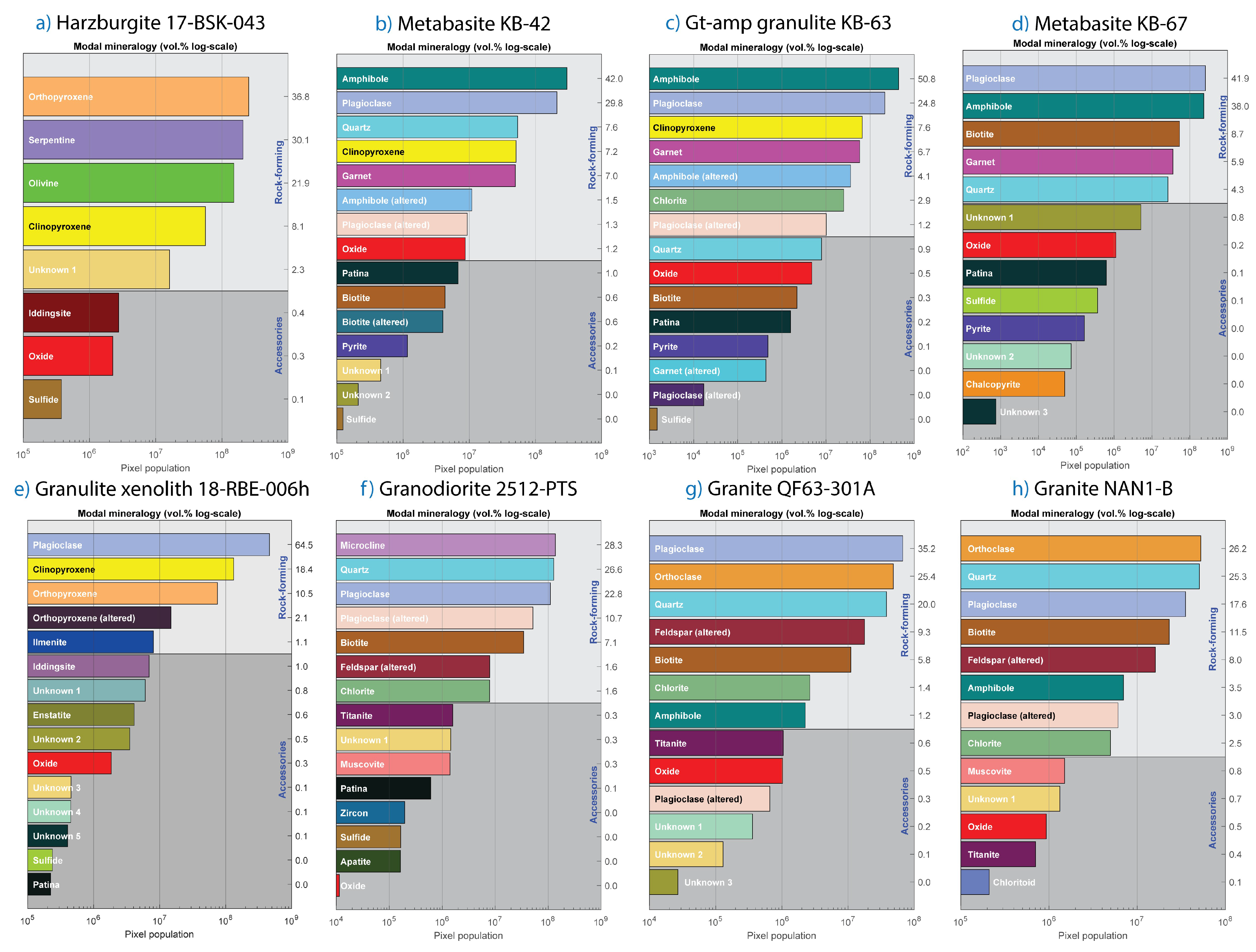
3.4. Phase Maps and Modal Mineralogy with Semantic Segmentation

Using a brief image annotation dataset for every thin section, QuPath was used to perform pixel classification (GeoJSON file output) using the aforementioned ray tracing image inputs (registered image stack). In conjunction with a programming bridge with MatLab, the optical phase maps were interpreted as modal mineralogy (%), showing phases in different colours (but without the application of one systematic colour legend). Figure 13 and Figure 14 present the semantic segmentation estimates. This yields meaningful modal mineralogies but represents mineral group masks without identifying grain instances. Thus, this approach misses information about rock texture and fabric, as it does not apply a grain boundary splitting approach, e.g., [16]. The legends of the maps show that similar to SEM-EDX-based phase segmentation, arbitrary decisions need to be made by the expert informing the training data. For example, altered plagioclase has a different optical appearance to fresh feldspar and the two can be distinguished even though in the original rock, they represented one phase. The legends also show that for accessory phases making up less than 0.5 volume % of the slide, optical identification was not always successful because the microscope is not equipped with the conoscopic abilities that would be needed to pin down the diagnostic optical properties. The appearance of the phase maps (Figure 13) also qualitatively highlights that phase recognition was most successful for the ultramafic rocks, followed by the mafic granulites, while the quartz and feldspar-rich granitoids show phase distribution that is apparently too intergrown. This is not due to lacking optical resolution but reflects the difficulty of visible-light distinction between quartz from feldspar and different feldspar types, as well as their alteration products.

4. Discussion

In this section, we first compare the optically derived phase proportions of the rock-forming minerals with the published modal mineralogy estimated by SEM-EDX. Next, we turn our attention to the difficulties posed by identifying (i.e., masking) fine-grained minerals, including the minor and accessory phases, with a pure optical and pixel-based approach. We show that in transmitted light, the 30–35 µm thickness of a thin section causes many optical complexities that are not seen in RL or in SEM-EDX-based phase maps where the electron beam interacts only to a depth of 1–2 µm. Then we discuss, in more detail, the additional insight gained from the various ray-tracing statistics and, finally, we discuss preliminary findings about combining the purely optical WSI modalities with chemical information, e.g., back-scatter-electron (BSE) maps.

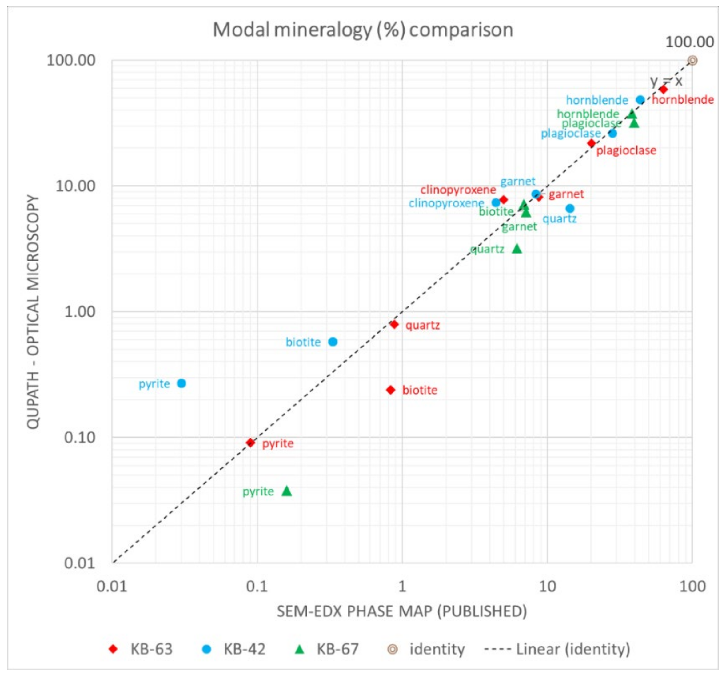
4.1. Comparison between Optical and SEM-EDX Modal Mineralogies

The image segmentation based on gamma-boosted RL, PPL-max, and XPL-max, shows the following level of correspondence with ground-truth modal mineralogy values: acceptable for ultramafic and mafic rocks; medium for granites; and low for granodiorites. The 1:1 trend in Figure 15 illustrates that the pixel population of minerals in mafic granulites is very similar between SEM-EDX phase maps (X-axis) [24], and ray tracing segmentation (Y-axis) for the rock-forming minerals. Sample KB-63 yielded an unforced trend line (y = 0.930x + 0.450) with R2 = 0.993 that improves in accuracy to y = 0.941x with R2 = 0.994 using the (0, 0) intercept. Sample KB-67 shows y = 0.898x − 0.240 with R2 = 0.985, and y = 0.891x with R2 = 0.987 using a forced intercept. Finally, sample 7KB-42 shows y = 1.05x − 0.424 with R2 = 0.964, and y = 1.03x with R2 = 0.971 using a forced intercept. For the samples in Figure 15, the percentage difference between the new method and the SEM-EDX phase mapping is best for plagioclase (11.5%), garnet (8%), and amphibole (6.9%) and worst for pyrite (95%), biotite (56%), and quartz (48.9%). Abundances of alkali-feldspar, calcite, ilmenite, Fe-oxide, apatite, titanite, and chlorite were difficult to compare in the selected samples because of scarcity and large uncertainty in at least one of the methods used. The section fringe artefacts (stage pocket edge, epoxy, etc.) might also have biased the optical mineralogy results, which could be improved by masking the appropriate area. For instance, xenolith 18-RBE-006h was not compared as the published values are for the xenolith only and not for the enclosing fine-grained basalt.
Not unexpectedly, accessory phases (<1 vol.%) show a larger mismatch. Some improvement in estimating the modal abundance of scarcer minerals would be possible if more time and effort were spent annotating and classifying them in the QuPath training dataset. However, we note that there is also a substantial difference in nominal spatial resolution. The SEM-EDX maps were obtained with 4.14 µm/px, while optical microscopy at 10× magnification yields 0.547 µm/px, making it hard to compare modalities in very fine-grained minerals.
In the studied rocks, the two main issues found with computer-assisted optical distinction were, first, to confidently distinguish between orthopyroxene-clinopyroxene (in granulites) and, second, between quartz-plagioclase-alkali feldspar (in granitoids). Other secondary issues are exposed and can be of variable severity, mainly depending on the desired number of segmentation classes and annotation training set quality. It was found that collectively attributing artefact pixels (dust, misregistered pixels, grain boundaries, surface scratches, and laser-ablation tracks on one of the studied granulites) to one unclassified class (e.g., ‘hole’, ‘glass-polish’, ‘patina’, etc.) minimizes their impact on overall modal estimates. We note that the annotation set for most rocks was kept to ca. 20 polygons per section without further improvements in the mineral masks in the interest of speed and ease of use.

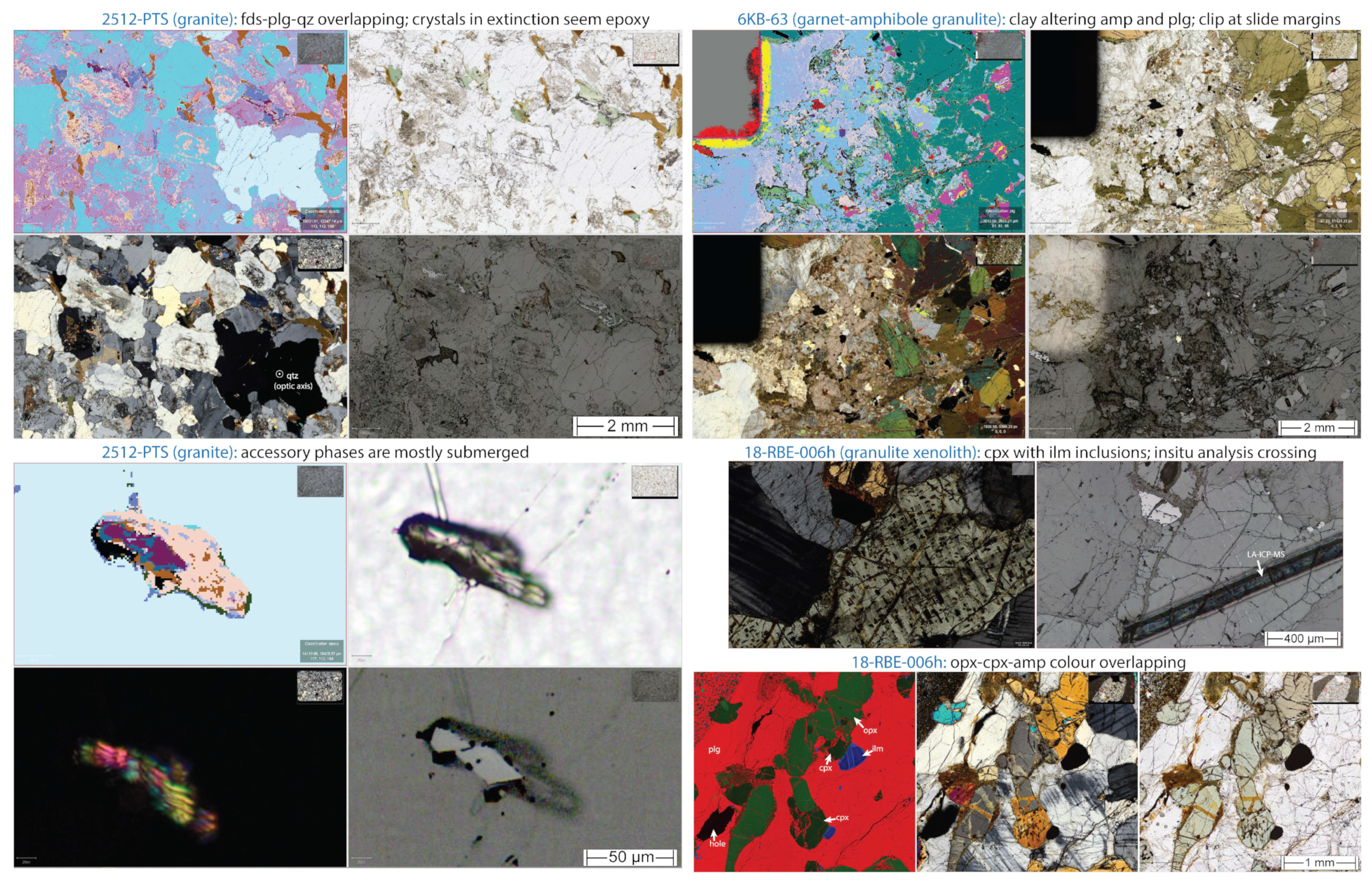
4.2. Examples of Challenging Segmentation of Optically Similar Phases and Very Fine-Grained Minerals

A catalogue of the more challenging situations for automated optical mineralogy is given in Figure 16, which shows the QuPath ‘multi-view’ canvasses. As expected, due to their lack of colour in PPL and similar low-order XPL interference colours, it is difficult to accurately distinguish between quartz, plagioclase, and alkali-feldspar without staining the feldspars. This is illustrated in Figure 16 with granodiorite 2512-PTS where the segmentation failed to define proper grain boundaries between microcline (linen colour), plagioclase (light blue), and quartz (cyan). By contrast, in the same FoV, biotite, chlorite, and muscovite were easily recognised (colour legend in Figure 14) on account of their characteristic combinations of PPL and XPL optical properties. With respect to the feldspars, the altered plagioclase is easier to recognize than the unaltered plagioclase, which in part was confused with quartz. A particular situation is displayed with a 2.5 mm anhedral quartz grain that happens to be perpendicular to the optical axis. In the segmentation, it was confused with the epoxy resin having full extinction in XPL-max, no variation in PPL-max, and irregular fractures in RL. A strength of the algorithm chain is that it finds grains in this optical orientation, which could be revisited by operators for producing interference figures and measuring the optic sign and/or angle (‘2V’) [8].
Of the studied samples, the granitoids are richest in abundance and diversity of accessory phases (apatite, zircon, titanite, oxides, etc.). Typically, accessory grains are quite small and expose an inherent limitation of transmitted light imaging of minerals in sections of 30–35 µm thickness. At the bottom-left of Figure 16, adjacent ca. 80 µm long prismatic zircon grains are enclosed in plagioclase along with a much thinner, highly acicular apatite crystal. The first thing to note is that in conventional transmitted light microscopy, it would not be obvious that the zircon grains are largely submerged within the thin section. However, RL (bottom-right panel) readily shows that the apatite is fully submerged, and only ca. 1/3 of the zircon crystals is exposed at the surface. Focusing initially only on the exposed zircon areas, the segmentation confused most of the pixels with titanite (purple in the phase map) and only recognised thin strips of zircon (shown in dark blue). The small stripe of zircon mingled with titanite shows the sensitivity of the Random Tree classifier, which was trained by re-weighting the unbalanced classes. The additional issue concerns the area of submerged zircon and apatite, which cause optical complexities, including colour overlap with plagioclase and altered plagioclase (magnolia colour). Furthermore, an example of a misregistration artefact is seen in the bottom-left panel (XPL-max), where ray tracing has propagated incorrectly along the grain boundaries, producing blurriness, which is obvious from seeing third-order interference colours next to a crystal in extinction.
At the top-right of Figure 16, one of the studied granulites (6KB-63) has experienced secondary alteration converting plagioclase, amphibole, and some garnet into clay minerals and other sheet silicates evidenced in XPL-min. In contrast, XPL-max is best suited for estimating the original minerals despite pseudomorphous replacement, for example, from altered plagioclase rimming less altered plagioclase. The phase map shows the difficulty of distinguishing altered amphibole (light blue) from plagioclase (light purple) and some sporadic clinopyroxene (yellow) ghosts that are misclassified and appear on top of altered amphibole. Therefore, the best pick of a ray tracing stack input is subject to trial and error, as discussed in the next section. Note also that grain contacts between amphibole (dark green) are ignored and/or misclassified as clinopyroxene in semantic segmentation. Moreover, the imaged area at the very edge of the slide (top-left) sitting above the stage holder next to the stage pocket edge (Figure 2) produced false medium reflectivity; that is, a dark area in transmitted light. Therefore, the segmentation was prone to failing in guessing the area as unclassified (grey) with false oxide (red) and clinopyroxene at the border. Most of these fringing areas can be masked within the MatLab script that interprets the phase map exports.
At the bottom-right of Figure 16, the pyroxene-plagioclase granulite xenolith (18-RBE-006h) panel shows clinopyroxene with prominent lamellar ilmenite exsolution along NW structural domains in transmitted light (XPL). When viewed at high zoom levels, the RL image shows that on the surface, the ilmenite only occupies a very small area as it outcrops as very fine grey planar crystals, with some forming peripherally around clinopyroxene. The RL image also shows a groove left after in situ laser-ablation analysis, which would necessarily have combined trace elements contained in the clinopyroxene and the ilmenite as the lamellae are much finer-grained than the diameter of the laser beam. Finally, the panel at the bottom illustrates a comparison between SEM-BSE, XPL-max, and unpolarised RL (right) on an area containing ortho- and clinopyroxene and plagioclase. The denser orthopyroxene appears in medium green false colour, while clinopyroxene (less dense) has a dark green colour in the recoloured BSE. The XPL-max image shows the birefringence overlap (1st-order orange) between the two pyroxenes at certain indicatrix orientations. In this situation, PPL-max (very bottom-right panel) was more successful at segmenting the two pyroxenes, whereas, including XPL-max, as required by the rest of the mineral assemblage, caused the algorithm to misidentify some ortho- as clinopyroxene.

4.3. Ray Tracing Insights

Ray tracing during virtual stage rotation uses descriptive statistics of the components of elliptically polarised light escaping sectioned mineral bottoms with (PPL) or without (XPL) crossing the analyser, which can be represented in images with integer (min, max, etc.) or double (e.g., std, pca) pixels. For segmentation, it is convenient to read pixels as absolute values that are rescaled within (1–99) percentiles to 24-bit RGB images. Note that this results in representations that are adaptable for different mineral assemblages but not specific mineral species between samples. Following petrographic observations within QuPath (used, in this instance, as an offline virtual microscope), the following main insights were gained from ray tracing:
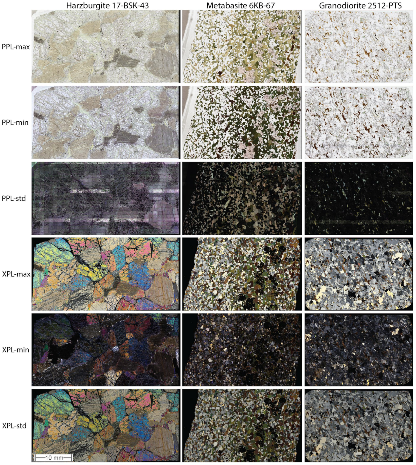
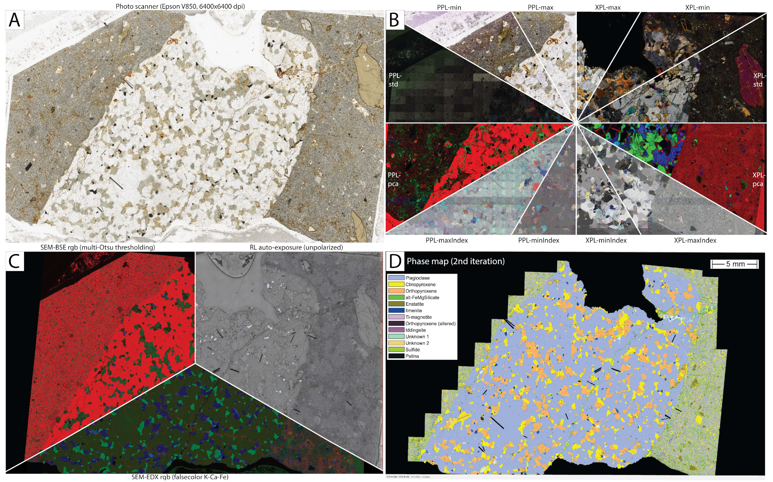
  • PPL-min: best at exposing strongly translucent minerals (weak colour), dark inclusions, and micro-fractures;
  • PPL-max: shows the pleochroism colour peak and slightly smoothens transparent mineral roughness due to the unpolished bottom of the section. This image orientation coincides with XPL-min due to the O-wave (isotropic) component behaviour;
  • PPL-std: picks out strongly pleochroic minerals. It is very susceptible to uncorrected residual shading. In perfectly unshaded WSI, PPL-std can reveal otherwise invisible image stitching issues. It also exposes micro-structures with ‘wobbling’ shadows;
  • XPL-min, e.g., [29]: displays mineral inclusions, micro-fractures, secondary alteration minerals within grains in extinction, and very low-angle contacts. It can solve the quartz colour overlap with plagioclase since quartz bands (metabasite 7KB-42) can appear in yellow and grey (not only grey), and also finds areas for producing interference figures;
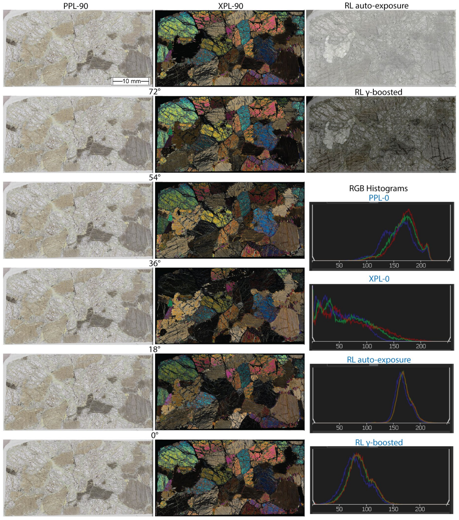
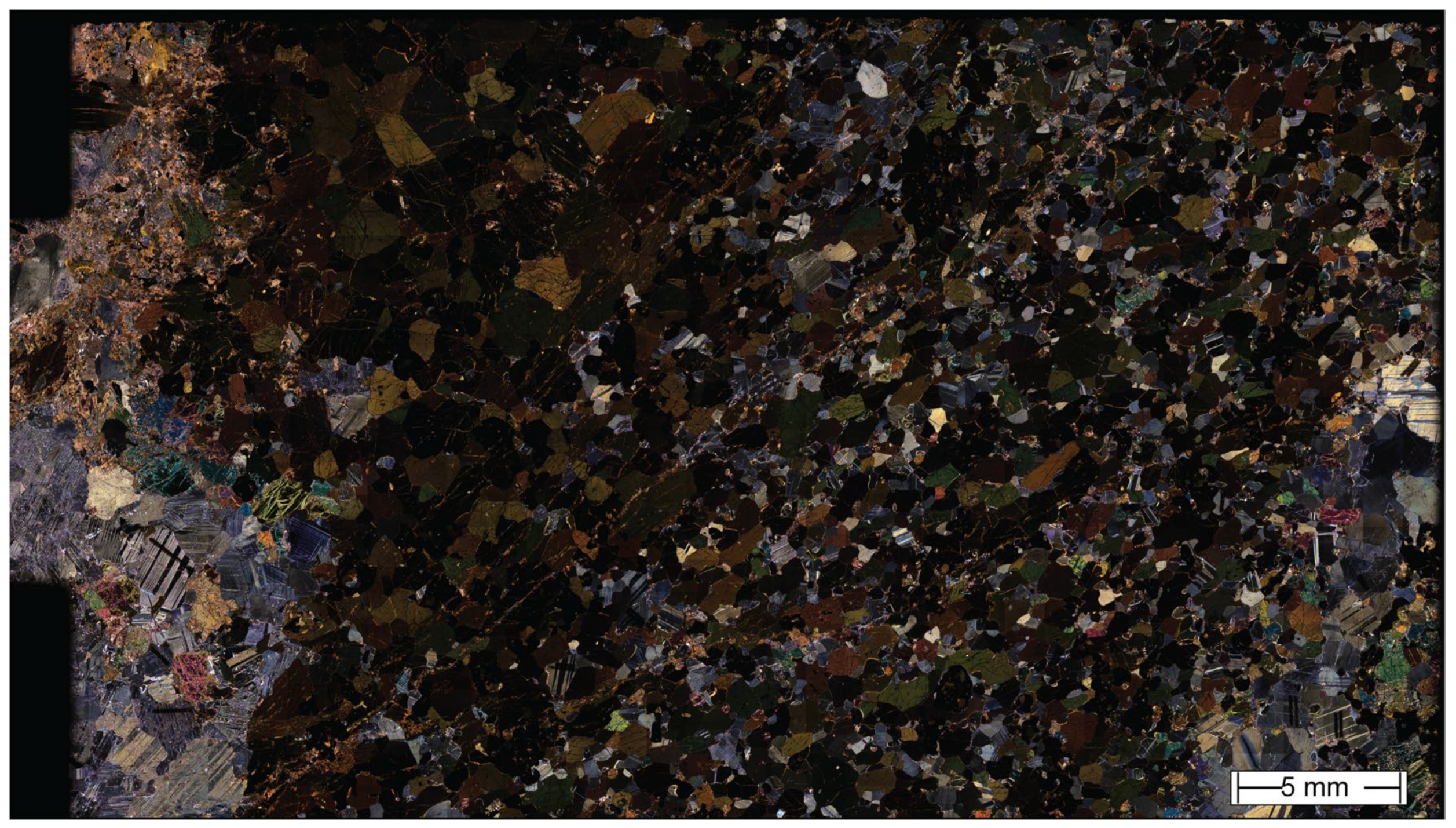
  • XPL-max and XPL-std, e.g., [30]: shows the approximate interference colour peak (not interpolated) of each pixel location that improves the rock texture visualisation. Therefore, slight colour intensity differences depend on grain crystallographic orientation, which might depend on rock fabric, but as shown with the last example in Figure 16, XPL-max can lead the segmentation algorithm to misidentify minerals that show a large range in birefringence (e.g., clinopyroxene);
  • PPL-pca: helps visualise the altered Fe-Mg silicate networks and halos shown in the xenolith basaltic matrix. Very slight colour differences are also observed depending on crystal orientation;
  • XPL-pca: highlights the grain boundaries and internal texture, such as twinning, fractures, and inclusion trails. The colouring mostly depends on the grain orientation and not on the mineral identity;
  • PPL-maxIndex or -minIndex: the initial polarisation setup has not captured the full 180° period in PPL. A new setup covering 0, 30, 60, 90, 120, and 150° has solved this issue and improved spectral homogeneity (applied only to 18-RBE-006h);
  • XPL-maxIndex or -minIndex: depending on the multi-pol step size, it can separate grains if they are oriented differently. It is useful for describing twinning and undulous extinction. As processing RGB channels works in the fourth-dimension, there is a chance of colouring the grains for certain indicatrix orientation that could become beneficial.
Observing mineral grains, ‘max’ and ‘min’ ray traces significantly reduce the outline of crystal twinning within single crystals and reduce the complexity if there are enough multi-pol steps. Previous workers identified the same benefits in using PPL-min, -max, -minIndex, XPL-max, and -maxIndex [17,31] and in using orthogonal traverses, e.g., [32], such as Figure 10, to understand the colour periodicity. XPL-pca and XPL-maxIndex (azimuthal orientation) show potential to contour grains, but they carry no information on the diagnostic wavelengths, while the XPL-range, e.g., [33] (XPL-max minus XPL-min), might produce coloured artefacts but conveniently darkens edges. Further images can be calculated, including incremental PCA in a single stack (RL, PPL, and XPL). This technique has a linear dependence on the variability in the feature space, and such variability does not relate to physical phenomena. Thus, future work will test deep sparse auto-encoders [34] that are non-linear and can be trained within a master sample collection mineralogy and image stack order (further generalised for all tiles), which might help reduce the embedded space dimensionality and improve QuPath performance.
The γ-boosted RL imaging has enhanced silicate and carbonate colour contrasts while widening the WSI histogram. However, the acquisition should carefully consider very reflective phases (e.g., pyrite and gold) that, in RGB histograms, are considerably separated from the bulk intensity mode of the non-reflective phases. Normally the brightness needs to be reduced to avoid oversaturation of the reflective phases to a point where still enabling observation of less-reflective areas (Figure 4 and Figure 5). For this reason, we opted to also acquire γ-boosted RL images, noting that the pixel values are not used for quantifying optical phenomena. To provide further insight into the capacity of using RL for improved segmentation, polarisation (RL-PPL and XPL) will need to be explored.

4.4. Combining Chemical Maps with Optical WSI (Second Iteration Phase Mapping)

The logical addition of more information to the stacks begins with either considering bulk mineral density (SEM-BSE) or the distribution of chemical constituents (element maps). An example of these two options is shown in Figure 17 for a thin section WSI of a granulite xenolith contained within fine-grained basalt. Density can be represented in a single layer, originally a grayscale BSE that can be non-linearly recoloured with thresholding techniques (see Supplementary Materials S1 (SEM-BSE greyscale recoloring by Multi-Otsu thresholding)). The resulting false-colour image encompasses many mineral properties (crystal lattice associations). In terms of chemical map WSI, it is most economical to generate a three-element map as a false-colour RGB, selecting a combination of three elements that best distinguish between phases that were difficult to tell apart from pure optical microscopy. Preliminary work with the inclusion of a high spatial resolution (~1 µm/px) SEM-BSE layer (Figure 17) to the ray tracing image stack) has improved the accuracy of the QuPath phase classification, with good results for the medium-grained granulite xenolith. However, the trial work has also revealed issues with slightly imperfect whole-slide image registration between the optical and SEM modalities. Therefore, with a greater number of microscopy modalities distinguishing fine-grained accessory minerals of less conspicuous features becomes increasingly difficult, which limits the image segmentation performance and textural analysis.
The pair-wise image registration was performed in Fiji with the ‘BigWarp’ plugin [35] using control-point image registration (20-point hexagonal grid on top of both images) and thin-plate spline transformation model to compensate for stage drift (large-scale cumulative offsets). The registered images were then re-imported into QuPath to apply the ‘Combiner’ plugin rescaling (upscale factor = 2). Follow-up visual inspection showed that the alignment between optical and SEM microscopy images was still not perfect, particularly in very fine-grained rocks, such as the xenolith basaltic matrix shown in Figure 17 and Figure 18C,D.
Therefore, to improve the second-iteration segmentation, prime-quality image stitching and alignment of the montages are a priority. Open-source software, such as Fiji ‘TrakEM2′ [36] or ‘MIST’ [37] plugins, are viable for tile-based navigation and globally optimised stitching of superior quality to proprietary software. Moreover, QuPath can also be utilised within the ‘Warpy’ software [38], allowing a three-step estimation of non-rigid transforms between confocal and TEM imagery, which might prove useful for localised tiling areas of challenging registration. Some of these issues and the ambiguity of knowing the most adequate image to act as a ‘fixed’ or ‘target’ could be resolved with the provision of a ground-truth geometry, for example, from a flatbed photo scan (perfect geometry).
Even for perfectly aligned images, it is safe to predict that some segmentation issues will remain. Most notably, it will remain difficult to contour very fine-grained minerals due to the ray trajectory within grains at non-perpendicular low-angle contacts causing a shadow ‘wobbling’ effect related to the ray internal reflection and intensity variations due to the dielectric metallic behaviour of the reflective minerals that polarize light into p- and s-waves along the resulting plane of incidence [39]. Navigating within QuPath, the shadowing is seen in PPL-std by observing the fracture networks that stand out in green within minerals that are not pleochroic (e.g., 18-RBE-006h and 17-BSK-043).
To further identify accessory minerals and improve on the truthful identification of fine-grained rock-forming minerals, a second iteration of the phase map is required. It is logical to consider importing chemical information from SEM-EDX and combining it with the first-iteration optical phase map. There are several paths towards achieving this step. The first is to run a WSI EDX scan and use the proprietary software to generate a purely SEM-based phase map, independent from the optical microscopy iteration #1 phase map. Some SEM-EDX software provides convenient report files along with the phase map that list the spectra for the identified compounds. This was explored with one trial and quickly identified several limitations. First, an EDX phase map can contain many more (>50) unclassified masks than the simpler optical microscopy iteration #1 phase list. Many of these unclassified masks are unlikely to correspond to actual phases, and their number depends on the selected binning factor, ‘grouping level’, and ‘boundary tolerance’. It is impossible to find an agreeable comparison of such large numbers of compound (unclassified) masks with the much lower expected number of phases reasonably expected to be present in most rocks.
There are many more pixels (billions) than mineral grains (hundreds of thousands) to be classified. To overcome this issue, the most economical approach would be to use the iteration #1 phase map to generate a list of x-y-coordinates to instruct the SEM-EDX system to target analysis. For example, in unevenly grained rocks, it makes limited sense to put rigid x-y EDX grids across the entire thin section because this will result in the acquisition of analyses on large grains that were already successfully identified with the iteration #1 phase map. Instead, the SEM-EDX should analyses should be targeting grains of uncertain mineralogy based on optical properties. Targeted SEM-EDX analysis, such as envisaged here, already exists in some proprietary software, for example, informed by SEM-BSE greyscale classes in TIMA [40]. However, the data reduction routines require selecting characteristic X-ray lines and/or producing spectral databases and validating (XRD and SEM-WDS), which is especially troublesome for complex samples and low elemental concentration (and contrasts).
The other approach is to resample the full-scale SEM-EDX phase map. This was trialled here with a communication script that lays out registered EDX grids on top of the WSI image stack. The two-step script occupies a 30 min routine that requires an input text file that the expert modifies with a desired regrouping of compounds into minerals that are verifiable by optical microscopy. The spectra report (*.pdf) is used for first-hand expert identification, and the mask files (*.tif) aid in geographical comparisons between classes and the multi-pol z-stacks in OlyVIA. Next, the EDX phase map is re-saved, registered (with BigWarp), and converted into a final grid that can easily be imported into QuPath because it can import ‘point’ annotations. The importing computing cost escalates quickly depending on the original binning factor of the map (converted into a grid). Nevertheless, the correlative routine (at a binning factor of 1) has improved our knowledge of the granulite xenolith hypersthene, augite and matrix orthopyroxene and altered Fe-Mg silicate of a reddish tone (also penetrating the xenolith and riming orthopyroxene). It also showed that the xenolith contained most of the apatite and ilmenite (only traces in the matrix), while the xenolith ilmenite lamellae were of titano-magnetite exsolution.
In summary, our initial assessments of combining WSI optical with SEM-derived information have yielded some promising results. The optical-mineralogy-based iteration #1 phase maps of typical fully crystalline rocks is substantially improved when information from BSE is added (e.g., the granulite xenolith shown in Figure 17D). For most rocks, this approach is expected to yield phase maps of comparable quality to SEM-EDX automated mineralogy with much lower SEM offline processing time requirements. However, in very-fine-grained rocks, apparently random misregistration was found, even when two very-well-registered sets of images were used. This implies that at least one set of images, albeit internally consistently registered and aligned, is deformed. Most likely, both sets of images contain long-range non-rigid deformation, and more work will be required to align optical and SEM-BSE image mosaics for targeting very fine objects. Moving on to adding SEM-EDX or -WDS information, the preliminary investigation shows that:
  • It will be most economical, in terms of both SEM instrument time and computational effort, to use the iteration #1 optical phase map to generate an x-y-coordinate list for targeted chemical analysis and to retrieve this information back into QuPath as ‘point’ annotation training data. However, this will not resolve the issue of not having achieved more sophisticated grain segmentation. Hence, prior scalable object-based segmentation will need to be developed. This will produce edge maps independent of the sub-grain structure (twinning, inclusions, fractures, etc.) Ongoing work is exploring this way of avoiding ‘mixels’ and improving correlative microscopy time per grain.
  • The SEM-EDX instrument software needs to provide full programming access to allow pre-setting strategic analytical grids beyond the auto-generated pre-segmentation already available to target accessory phases, avoid cracks, and refrain from oversampling large homogeneous grains.
  • In terms of manufacturing, it would be beneficial to reach a consensus on standardised thin-section dimensions and stages; for instance, stage drift could be minimised upstream using motion-estimation-corrected trajectories with live feedback from faster and more sensitive detectors. This would significantly help register WSI from different modalities.

5. Summary and Outlook

This study proposes two main steps towards quantitative digital petrographic microscopy. The first is to reduce multi-angle polarisation WSI (here six each in PPL and XPL) into single new statistical representation images with ray tracing. This can both greatly reduce the effects of grain orientation-dependent anisotropy (e.g., via -max or -min projections) or distinguish between strongly and modestly anisotropic phases. The second step is a pilot software pipeline within which images are corrected and registered and in which ray tracing is performed before semantic image segmentation.
Within the studied rocks of known mineralogy and modal abundance, two main future challenges have been identified using QuPath navigation, namely the alkali feldspar-plagioclase-quartz and orthopyroxene-clinopyroxene-amphibole colouring overlaps. In addition, the areas where ‘live’ segmentation has shown to be more doubtful are grain contacts. These can be outlined with the ‘wand’ tool in γ-boosted RL, distinguishing low-reflectivity silicates, clay alteration clots, opaques, and outcropping fine-grained accessory phases (at 40×). Notably, the immersive petrographic experience has been further improved by recolouring SEM-BSE, dimensionality reduction, and image pyramid segmentation that allows navigation on fewer images. Such virtual microscopes allow better documenting petrographic findings than representative digital microscope photographs.
The study has revealed that petrographic WSI image analysis will progress in a sequence of steps in which information additional to pure optical micrographs is required. The first iteration phase map with the analysis of RL and ray-traced PPL and XPL representations is a solid starting point of negligible cost and requirements against SEM-EDX [41]. The resulting follow-up iterations have shown greater accuracy and potentially could quantify accessory phases provided image stitching and pair-wise image registration is prioritised. Meanwhile, for all but the finest-grained rocks and overlapping/low birefringence minerals (e.g., apatite), the logical next addition is a high-resolution SEM-BSE image as well as SEM-EDX analyses, guided by optical WSI object maps.
Image segmentation of geological thin sections has so far resorted to simple rock types that are often sedimentary, monomineralic, medium-grained, and contain uniaxial phases of low (but distinctive) anisotropy, generating dichroic and interference colours against a dark uniform background (matrix, epoxy resin, etc.). It is no surprise that sandstones and heavy detritus have become successful examples of the digital characterisation of porosity with dyed injected resins and particle detection. For holocrystalline igneous (here peridotites to granites) and metamorphic rocks, we require much more complex image feature engineering. These rocks hold promise to address questions of greater ambition. For example, mineral grain maps hold the potential to tackle questions such as which phases constitute an equilibrium assemblage, which minerals belong to various alteration assemblages, and what are the mutual grain contact, e.g., [42], and size relationships despite shape similarity.
Finally, the remaining developing priorities are perfect image registration and object-based segmentation (identifying true crystal faces). Image annotation and object description and classification, e.g., [43], are more feasible with a hybrid-learning approach, where user annotations are augmented by pre-segmentation [44]. In terms of mineralogical modelling, one future goal is to model the refractive index in 3D and to overcome the major limitation of interference colour overlap. The first principle spectral modelling of multi-pol images (Supplementary Materials S1 (Fourier spectral modeling)) can reduce the data to orientation and pole maps [45] that may eventually overcome some of these limitations.

Supplementary Materials

The supporting information providing details into the instrument calibration and image analysis pipeline can be downloaded at: https://www.mdpi.com/article/10.3390/min13020156/s1, Supplementary Materials S1: Methodology details; Supplementary Materials S2: Visualizing whole-slide images. References [46,47,48,49,50,51,52] are listed in the Supplementary Materials S1 and S2.

Author Contributions

Conceptualisation, project administration, visualisation, M.A.A.Z. and B.S.K.; methodology, software, investigation, data curation, writing—original draft preparation, formal analysis, validation, M.A.A.Z.; supervision, writing—review and editing, B.S.K. All authors have read and agreed to the published version of the manuscript.

Funding

This research was supported by a QUT South American Scholarship (STHAM) that sponsored the PhD tuition fees and living cost.

Data Availability Statement

The slide scanner data of two thin sections can be accessed via the ‘database’ feature in the free web-based OlyVIA slide viewer. Instructions for accessing the two slides can be found in Supplementary Materials S2. The code of the pipeline is provided within the ‘Acevedo&Kamber’ folder (https://github.com/marcoaaz (accessed on 16 January 2023)). Interested readers can make use of the recommendations about VS200 upgrades and pipeline trials within Supplementary Materials S1 (Future work recommendations).

Acknowledgments

The data reported in this paper were obtained at the Central Analytical Research Facility (CARF). We acknowledge funding from QUT’s Strategic Major Equipment Program for the VS200. The CARF staff are thanked for their support, flexibility during the experimentation period, and software inductions. Robert Emo is thanked for granting access to the SEM databases of his thin sections. We are grateful to Sandrine Roy and Tong Wu from Evident (Olympus) Australia, who provided on- and off-site VS200 support and who coordinated the modifications of the instrument with the factory. We thank the three journal reviewers and the guest editor for their suggestions for improvement. Finally, our thanks go to the bioinformatics developer community (https://forum.image.sc/ (accessed on 16 January 2023)) on whose mostly anonymous open-source contributions our image analysis work is built.

Conflicts of Interest

The authors declare no conflict of interest. The funders had no role in the design of the study; in the collection, analyses, or interpretation of data; in the writing of the manuscript, or in the decision to publish the result.

References

  1. Gunter, M.E. The Polarized Light Microscope: Should We Teach the use of a 19th Century Instrument in the 21st Century? J. Geosci. Educ. 2004, 52, 34–44. [Google Scholar] [CrossRef]
  2. Kile, D.E. The Universal Stage: The Past, Present, and Future of a Mineralogical Research Instrument. Geochem. News 2009, 140, 1–21. [Google Scholar]
  3. Frost, M.J. Refractive Index. In Mineralogy; Springer: Berlin/Heidelberg, Germany, 1983; pp. 438–441. [Google Scholar]
  4. Wallace, C.T.; St Croix, C.M.; Watkins, S.C. Data management and archiving in a large microscopy-and-imaging, multi-user facility: Problems and solutions. Mol. Reprod. Dev. 2015, 82, 630–634. [Google Scholar] [CrossRef] [PubMed] [Green Version]
  5. Marée, R.; Rollus, L.; Stevens, B.; Hoyoux, R.; Louppe, G.; Vandaele, R.; Begon, J.-M.; Kainz, P.; Geurts, P.; Wehenkel, L. Collaborative analysis of multi-gigapixel imaging data using Cytomine. Bioinformatics 2016, 32, 1395–1401. [Google Scholar] [CrossRef] [PubMed] [Green Version]
  6. Saalfeld, S. Computational methods for stitching, alignment, and artifact correction of serial section data. Methods Cell Biol. 2019, 152, 261–276. [Google Scholar] [CrossRef]
  7. Giesen, C.; Wang, H.A.O.; Schapiro, D.; Zivanovic, N.; Jacobs, A.; Hattendorf, B.; Schüffler, P.J.; Grolimund, D.; Buhmann, J.M.; Brandt, S.; et al. Highly multiplexed imaging of tumor tissues with subcellular resolution by mass cytometry. Nat. Methods 2014, 11, 417–422. [Google Scholar] [CrossRef]
  8. Raith, M.M.; Raase, P. Thin Section Microscopy: A Comprehensive Guide. Available online: http://nationalpetrographic.com/thin-section-microscopy-a-comprehensive-guide.html (accessed on 24 May 2022).
  9. Heilbronner, R.P.; Pauli, C. Integrated spatial and orientation analysis of quartz c-axes by computer-aided microscopy. J. Struct. Geol. 1993, 15, 369–382. [Google Scholar] [CrossRef]
  10. Heilbronner, R. Automatic grain boundary detection and grain size analysis using polarization micrographs or orientation images. J. Struct. Geol. 2000, 22, 969–981. [Google Scholar] [CrossRef]
  11. Ng, A. Sparse Autoencoder; CS294A Lecture Notes; Stanford Univ.: Stanford, CA, USA, 2011; Available online: https://web.stanford.edu/class/cs294a/sparseAutoencoder_2011new.pdf (accessed on 28 January 2022).
  12. Matthew, A. A Revolution in Quantitative Petrography_Digitization and Automation with Machine Learning; Carl Zeiss Microscopy GmbH: Pleasanton, CA, USA, 2021; Available online: https://www.zeiss.com/microscopy/en/c/rwm/22/natres/quantitative-petrography/quantitative-petrography.html (accessed on 16 January 2023).
  13. Koh, E.J.Y.; Amini, E.; McLachlan, G.J.; Beaton, N. Utilising convolutional neural networks to perform fast automated modal mineralogy analysis for thin-section optical microscopy. Miner. Eng. 2021, 173, 107230. [Google Scholar] [CrossRef]
  14. Dickson, J.A.D. Carbonate identification and genesis as revealed by staining. J. Sediment. Res. 1966, 36, 491–505. [Google Scholar] [CrossRef]
  15. Grove, C.; Jerram, D.A. jPOR: An ImageJ macro to quantify total optical porosity from blue-stained thin sections. Comput. Geosci. 2011, 37, 1850–1859. [Google Scholar] [CrossRef]
  16. Roduit, N. JMicroVision: Un Logiciel d‘Analyse d‘Images Pétrographiques Polyvalent. Monograph, Section des Sciences de la Terre, Université de Genève 2007. Available online: http://archive-ouverte.unige.ch/unige:468 (accessed on 16 January 2023).
  17. Fueten, F. A computer-controlled rotating polarizer stage for the petrographic microscope. Comput. Geosci. 1997, 23, 203–208. [Google Scholar] [CrossRef]
  18. Ogliore, R.; Jilly-Rehak, C. Gigapixel Optical Microscopy for Meteorite Characterization. Planet. Sci. 2013, 2, 1023. [Google Scholar] [CrossRef] [Green Version]
  19. Axer, M.; Strohmer, S.; Gräßel, D.; Bücker, O.; Dohmen, M.; Reckfort, J.; Zilles, K.; Amunts, K. Estimating Fiber Orientation Distribution Functions in 3D-Polarized Light Imaging. Front. Neuroanat. 2016, 10, 40. [Google Scholar] [CrossRef] [Green Version]
  20. Koike-Tani, M.; Tani, T.; Mehta, S.B.; Verma, A.; Oldenbourg, R. Polarized light microscopy in reproductive and developmental biology. Mol. Reprod. Dev. 2015, 82, 548–562. [Google Scholar] [CrossRef] [Green Version]
  21. Pirnstill, C.W.; Cote, G.L. Malaria Diagnosis Using a Mobile Phone Polarized Microscope. Sci Rep 2015, 5, 13368. [Google Scholar] [CrossRef] [Green Version]
  22. Buchrieser, J.; Dufloo, J.; Hubert, M.; Monel, B.; Planas, D.; Rajah, M.M.; Planchais, C.; Porrot, F.; Guivel-Benhassine, F.; Van der Werf, S.; et al. Syncytia formation by SARS-CoV-2-infected cells. EMBO J. 2020, 39, e106267. [Google Scholar] [CrossRef]
  23. Emo, R.B.; Kamber, B.S. Evidence for highly refractory, heat producing element-depleted lower continental crust: Some implications for the formation and evolution of the continents. Chem. Geol. 2021, 580, 120389. [Google Scholar] [CrossRef]
  24. Emo, R.B.; Kamber, B.S. A Reconstitution Approach for Whole Rock Major and Trace Element Compositions of Granulites from the Kapuskasing Structural Zone. Minerals 2020, 10, 573. [Google Scholar] [CrossRef]
  25. Bankhead, P.; Loughrey, M.B.; Fernandez, J.A.; Dombrowski, Y.; McArt, D.G.; Dunne, P.D.; McQuaid, S.; Gray, R.T.; Murray, L.J.; Coleman, H.G.; et al. QuPath: Open source software for digital pathology image analysis. Sci. Rep. 2017, 7, 16878. [Google Scholar] [CrossRef] [Green Version]
  26. Caja, M.Á.; Pena, A.; Campos, J.; Diego, L.; Tritlla, J.; Bover-Arnal, T.; Martín-Martín, J.D. Image Processing and Machine Learning Applied to Lithology Identification, Classification and Quantification of Thin Section Cutting Samples. In Proceedings of the SPE Annual Technical Conference and Exhibition, Calgary, AL, Canada, 30 September–2 October 2019. Paper SPE-196117-MS 2019. [Google Scholar]
  27. Bankhead, P. Analyzing Fluorescence Microscopy Images with ImageJ; Queen’s University Belfast: Belfast, UK, 2014. [Google Scholar]
  28. Schneider, C.A.; Rasband, W.S.; Eliceiri, K.W. NIH Image to ImageJ: 25 years of image analysis. Nat. Methods 2012, 9, 671–675. [Google Scholar] [CrossRef] [PubMed]
  29. Yesiloglu-Gultekin, N.; Keceli, A.S.; Sezer, E.A.; Can, A.B.; Gokceoglu, C.; Bayhan, H. A computer program (TSecSoft) to determine mineral percentages using photographs obtained from thin sections. Comput. Geosci. 2012, 46, 310–316. [Google Scholar] [CrossRef]
  30. Jungmann, M.; Pape, H.; Wißkirchen, P.; Clauser, C.; Berlage, T. Segmentation of thin section images for grain size analysis using region competition and edge-weighted region merging. Comput. Geosci. 2014, 72, 33–48. [Google Scholar] [CrossRef]
  31. Fueten, F.; Mason, J. An artificial neural net assisted approach to editing edges in petrographic images collected with the rotating polarizer stage. Comput. Geosci. 2007, 33, 1176–1188. [Google Scholar] [CrossRef]
  32. Zhou, Y.; Starkey, J.; Mansinha, L. Identification of Mineral Grains in a Petrographic Thin Section Using Phi- and Max-Images. Math. Geol. 2004, 36, 781–801. [Google Scholar] [CrossRef]
  33. Zhang, Y.; Zhong, H.-R.; Zhang, X.; Gao, S.-C.; Zhang, D. Orthogonal microscopy image acquisition analysis technique for rock sections in polarizer angle domain. J. Struct. Geol. 2020, 140, 104174. [Google Scholar] [CrossRef]
  34. Thomas, S.A. Fast Data Driven Estimation of Cluster Number in Multiplex Images using Embedded Density Outliers. In Proceedings of the 2022 IEEE Conference on Computational Intelligence in Bioinformatics and Computational Biology (CIBCB), Ottawa, ON, Canada, 15–17 August 2022. [Google Scholar]
  35. Bogovic, J.A.; Hanslovsky, P.; Wong, A.; Saalfeld, S. Robust registration of calcium images by learned contrast synthesis. In Proceedings of the 2016 IEEE 13th International Symposium on Biomedical Imaging (ISBI), Prague, Czech Republic, 13–16 April 2016; pp. 1123–1126. [Google Scholar] [CrossRef] [Green Version]
  36. Cardona, A.; Saalfeld, S.; Schindelin, J.; Arganda-Carreras, I.; Preibisch, S.; Longair, M.; Tomancak, P.; Hartenstein, V.; Douglas, R.J. TrakEM2 software for neural circuit reconstruction. PLoS One 2012, 7, e38011. [Google Scholar] [CrossRef] [Green Version]
  37. Chalfoun, J.; Majurski, M.; Blattner, T.; Bhadriraju, K.; Keyrouz, W.; Bajcsy, P.; Brady, M. MIST: Accurate and Scalable Microscopy Image Stitching Tool with Stage Modeling and Error Minimization. Sci. Rep. 2017, 7, 4988. [Google Scholar] [CrossRef] [Green Version]
  38. Chiaruttini, N.; Burri, O.; Haub, P.; Guiet, R.; Sordet-Dessimoz, J.; Seitz, A. An Open-Source Whole Slide Image Registration Workflow at Cellular Precision Using Fiji, QuPath and Elastix. Front. Comput. Sci. 2022, 3, 780026. [Google Scholar] [CrossRef]
  39. Gunter, M.E. Polarized light reflection from minerals; a matrix approach. Eur. J. Mineral. 1989, 1, 801–814. [Google Scholar] [CrossRef]
  40. Hrstka, T.; Gottlieb, P.; Skala, R.; Breiter, K.; Motl, D. Automated mineralogy and petrology—Applications of TESCAN Integrated Mineral Analyzer (TIMA). J. Geosci. 2018, 63, 47–63. [Google Scholar] [CrossRef] [Green Version]
  41. Maitre, J.; Bouchard, K.; Bédard, L.P. Mineral grains recognition using computer vision and machine learning. Comput. Geosci. 2019, 130, 84–93. [Google Scholar] [CrossRef]
  42. Higgins, M. Advances in the textural quantification of crystalline rocks. Geosci. Can. 2015, 42, 263–270. [Google Scholar] [CrossRef] [Green Version]
  43. Latif, G.; Bouchard, K.; Maitre, J.; Back, A.; Bédard, L.P. Deep-Learning-Based Automatic Mineral Grain Segmentation and Recognition. Minerals 2022, 12, 455. [Google Scholar] [CrossRef]
  44. Yu, J.; Wellmann, F.; Virgo, S.; von Domarus, M.; Jiang, M.; Schmatz, J.; Leibe, B. Superpixel segmentations for thin sections: Evaluation of methods to enable the generation of machine learning training data sets. Comput. Geosci. 2023, 170, 105232. [Google Scholar] [CrossRef]
  45. Goodchild, J.S. Geological Image Processing of Petrographic Thin Sections Using the Rotating Polarizer Stage. Brock University. 1998. Available online: http://hdl.handle.net/10464/1891 (accessed on 9 July 2009).
  46. Ross, D. A.; Lim, J.; Lin, R.-S.; Yang, M.-H. Incremental Learning for Robust Visual Tracking. Int. J. Comput. Vis. 2008, 77, 77–125. [Google Scholar] [CrossRef]
  47. Schroeder, A. B.; Dobson, E. T. A.; Rueden, C. T.; Tomancak, P.; Jug, F.; Eliceiri, K. W. The ImageJ ecosystem: Open-source software for image visualization, processing, and analysis. Protein Science 2021, 30, 234–249. [Google Scholar] [CrossRef]
  48. Cupitt, J.; Martinez, K. VIPS: An imaging processing system for large images. Proc. SPIE—Int. Soc. Opt. Eng. 1996, 1663. [Google Scholar] [CrossRef] [Green Version]
  49. Otsu, N. A Threshold Selection Method from Gray-Level Histograms. IEEE Trans. Syst. Man Cybern. 1979, 9, 62–66. [Google Scholar] [CrossRef] [Green Version]
  50. Gunter, M. E. Refractometry by Total Reflection; Virginia Polytechnic Institute and State University: Blacksburg, VA, USA, 1987. [Google Scholar]
  51. Sørensen, B. E. A revised Michel-Lévy interference colour chart based on first-principles calculations. Eur. J. Mineral. 2013, 25, 5–10. [Google Scholar] [CrossRef]
  52. Axer, M.; Graessel, D.; Kleiner, M.; Dammers, J.; Dickscheid, T.; Reckfort, J.; Huetz, T.; Eiben, B.; Pietrzyk, U.; Zilles, K.; et al. High-Resolution Fiber Tract Reconstruction in the Human Brain by Means of Three-Dimensional Polarized Light Imaging. Front. Neuroinformatics 2011, 5, 34. [Google Scholar] [CrossRef] [PubMed]
Figure 1. VS200 ST research slide scanner components. (A) The fundamental parts (top-left) are referenced (red lines) to the sketch of the base unit without housing panels (top-right). (B) The part diagrams (bottom-right) point out two possible optical paths (bottom-left) showing the source LED lamps. Copyright: Modified from Installation Manual VS200, Olympus.
Minerals 13 00156 g001
Figure 2. VS200 setup photos. (A) Sample chamber without sample tray showing components. The upper half of the optical axis is shown in dashed yellow lines. (B) Slide trays with the calibrating samples inserted in the long (pocket #3: Si semi-conductor wafer; 4: vs. calibrating sample; 5: biotite-garnet gneiss) and short (pocket #3: white label; 4 and 5: quartz crystals) trays.
Minerals 13 00156 g002
Figure 3. Example of VS200 optical performance in transmitted (PPL-90 and XPL-90) and reflected (RL unpolarised) light compared to a corresponding false-colour SEM-BSE image. From top to bottom (10×: 0.547; 20×: 0.273; 40×: 0.137 µm/px), the image shows a small area of a pyroxene-plagioclase granulite xenolith within a basalt (overview at bottom-right). In PPL, the decreasing depth-of-field at greater spatial resolutions is evident. In RL, the similarity of grain shapes is expected to be best in the recoloured SEM-BSE (Supplementary Materials for details). Sample 18-RBE-006h [23].
Minerals 13 00156 g003
Figure 4. Whole-slide images in plane polarized (PPL) (left) and cross-polarized light (XPL) (centre) in multi-angle polarisation showing 18° steps of slight pleochroism and vivid interference colours of a coarse-grained harzburgite with olivine, pyroxene (ol > opx > cpx), spinel, and alteration products. Two unpolarised reflected light (RL) images (top-right) are obtained, one with standard illumination and the other with the gamma value boosted (second on the top-right). This allows us to better distinguish different silicates in RL, as seen in the histograms (bottom-right). Sample ID: 17-BSK-043.
Minerals 13 00156 g004
Figure 5. Flowchart of the image analysis pipeline (option A) showing the main steps (blue squares), outputs (light orange squares), and deployed software (logos) for semantic segmentation. In Step 1, the images are uploaded to the server in proprietary format (*.vsi). Windows and Linux operating systems (OS) are utilised using packages detailed in the Supplementary Materials S1.
Minerals 13 00156 g005
Figure 6. QuPath image annotation on a powerful laptop (top-left) using the user-friendly annotation toolbar to generate internal GeoJSON files (top-centre) that describe the drawn polygons for the selected RL γ-boosted image (main picture). The tools use the visible layers (right panel) that can be toggled for convenience, helping the ‘wand’ tool for precise contouring of grains. The yellow square shows the field of view of Figure 7. Sample: harzburgite 17-BSK-043.
Minerals 13 00156 g006
Figure 7. QuPath platform using a multi-view canvas (2 × 2) with the ray tracing image stack overlaid by ‘live’ segmentation (top-left). The views show PPL-max (top-right), XPL-max (bottom-left), and RL γ-boosted (bottom-right) to give a petrographer views across all relevant modalities. The ‘Pixel classifier’ is operated to improve the labelled annotation set and to define classes for parametrised supervised clustering (centre sub-menu) following the mineral library (top-left tab: ‘Annotations’). The graphical user interface (GUI) navigates and updates the segmentation on each pyramid block (see Figure 8) of the combined image while reading annotations, calculating feature maps, and enabling the saving of the WSI semantic segmentation maps.
Minerals 13 00156 g007
Figure 8. QuPath ‘Pixel classifier’ workflow on the registered image stack (top) that is split into red-green-blue image layers (RGB) and then processed block-wise. The multi-scale feature map calculation (blue box inset) uses filtering for all selected channels. This helps find characteristic features with a random trees model during prediction. A loop reconstructs the phase map for each pixel and block (bottom-right). Sample ID: granulite-facies metabasite 7KB-42.
Minerals 13 00156 g008
Figure 9. Imaging of a hornblende granulite. (A) Whole-slide images in RL auto-exposure and γ-boosted marking the position of a ROI (red square) (top-left) and RGB histograms of PPL-0, XPL-0, and both RL (bottom-left). RL γ-boosting allows for better distinguishing of dielectric minerals of low reflectivity. (B) Schematic drawing shows ray tracing in an image patch stack at five different sample locations (vertical yellow lines) of distinct mineralogy. The two typical image dimensionality options (bottom-right) are specified. Sample ID: KB-67.
Minerals 13 00156 g009
Figure 10. Orthogonal views of Figure 9 stack (pyramidal level = 0) of the hornblende granulite KB-67. The PPL-36 (top-left) and XPL-18 (middle-right) positions illustrate the mineralogy. Five pixels of distinct mineralogy (biotite 1 and 2, plagioclase, garnet, and chlorite) are marked (blue stars) for each modality (RL, PPL, XPL) and orientation. Colour gradients within the orthogonal traverses are arranged left–right (vertical) and top–bottom (horizontal). The change in PPL and XPL colour is seen as a gradient as the stage is virtually rotated. ROI RGB spectra at 180 (PPL) steps and six steps (XPL) are shown at the bottom with ideal spectral fits to 180 (PPL) and 90° (XPL) periods.
Minerals 13 00156 g010
Figure 11. Ray tracing for PPL and XPL whole-slide images in ultra-mafic, mafic, and felsic rocks showing the mutual relationships between mineralogy and statistical measures (maximum, minimum, and standard deviation). The sample names are given at the top.
Minerals 13 00156 g011
Figure 12. XPL-min image of granulite-facies metabasite KB-63. It allows seeing areas of clay (prominently in the top-left) altering plagioclase, amphibole, and garnet (possibly kelyphite). Further, note the clay-filled micro-fractures that are oriented NE across the thin section. The sub-grain structural complexity of plagioclase can also be interpreted in XPL-min.
Minerals 13 00156 g012
Figure 13. Optical phase maps of the image stacks (RL γ-boosted, PPL-max, and XPL-max). Visually, the fidelity is better in ultra-mafic and mafic rocks. It generally decreases towards felsic compositions due to pyroxenes and quartz-feldspar colour overlaps. The prediction scales of the maps (2 × 2 px: (af) maps, and 4 × 4 px: (g,h) maps) were set according to the visual quality assessment (iteration #1), see the colour legends in Figure 14. The published EDX phase maps are available for (bd) in [24] and e in [23].
Minerals 13 00156 g013
Figure 14. Legends and volume (%) modal abundance plots for the phase maps shown in Figure 13. The X-axis shows the pixel population (logarithmic) for easy comparison between the order of magnitude, whereas the Y-axis shows the conversion to volume % values for each phase. Phases for which identification was equivocal were tagged as ‘unknown’ or were named with broad mineral family names (oxide, sulphide, altered, etc.). The identification could be refined by adding chemical information.
Minerals 13 00156 g014
Figure 15. Modal mineralogy comparison of the segmentation from ray tracing stack and the SEM-EDX phase maps of metabasites [24]. The volume % abundance was weighted by nominal mineral densities. Note the logarithmic scale of the axes. Rock-forming minerals fit better to the 1:1 line (not the log-log scale) than accessory phases. Several phases identified in Figure 14 were omitted from the plot for clarity.
Minerals 13 00156 g015
Figure 16. QuPath showing challenges in the image analysis methodology with optical microscopy (iteration #1) on thin sections. The granitoid sample panels (left) are shown in logical ‘multi-view’ canvas order (top-left: phase map, bottom-left: XPL-max, top-right: PPL-max, and bottom-right: RL γ-boosted). The granulite (top-right) illustrates challenging secondary sheet silicate segmentation near the section margin. The pyroxene-plagioclase granulite xenolith (bottom-right) displays the difficulty of separating orthopyroxene from clinopyroxene depending on crystallographic orientation.
Minerals 13 00156 g016
Figure 17. Visual cross-referencing between a regular photo scan (A), ray tracing products (B), and electron microscopy (C) and a phase map (iteration #2) with a colour legend (D). Iteration #2 incorporated recoloured SEM-BSE and the -EDX ‘TruMap’ stack (27 characteristic X-ray lines) principal component analysis (PCA) to the ray tracing stack for improving segmentation accuracy. This has helped resolve the distinction between pyroxenes within the xenolith. The output map intersects have defined a smaller sample area (15 selectable channels, evidencing areas filled with alteration minerals, fracturing, epoxy, and prior laser ablation grooves). Pyroxene-plagioclase granulite xenolith 18-RBE-006h.
Minerals 13 00156 g017
Figure 18. QuPath zoom-in to 10× whole-slide image (WSI) of Figure 17. (A): iteration #1 phase map comparison alongside detailed RL image (B). This shows the imperfect distinction between the two pyroxenes. (C): Image overlay on medium-grained xenolith showing perfect image registration between SEM-BSE (40% transparency) and RL, which contain complementary information. (D): Contact between xenolith and basalt matrix illustrating random pixel offsets (top-left and bottom-right) due to intrinsic deformation within montages. Top-right inlets show fields-of-view (FoV) locations. Sample ID: 18-RBE-006h.
Minerals 13 00156 g018
Table 1. Repurposed VS200 calibration items and parts.
Calibration ItemOptical Light Path (Camera at the Top)Illumination Modality (Detailed Scan)Label Scan
BrightfieldPlane PolarisedCross-PolarisedReflected Light
VS Olympus calibration slide v2.0stage XYZ calbration, distortion, rotation, objective XY shift, parfocality, etc.shading (dark-field and flat-field)WB, shading
Bt-gt gneiss WB targeting epoxyorientation targeting biotite, WB targeting epoxyorientations cross-polarisation targeting garnet, WB targeting quartz
Semi-conductor silicon wafer (bluish color) shading (unfocusing dust)
Natural quartz slide (yellowish color, nearly perpendicular to C-axis) shading (unfocusing inclusions or dust)
White label (pasted on glass slide) WBWB, shading
Added part (not default):
Objective PLN 2× (achromat) X (overview scan) X
Objectives MPLFLN 10× and 40× (no cover glass semi-apochromat)XXXXX
Objective MPLAPON 20× LEXT (no cover glass plan-apochromat)XXXXX
pT-100 LED (CoolLED) X
Mounted wire grid polariser φ = 25 mm for 420–700 nm. Installed within U-FDICT cubes of IX3 (6 units) X
Ø1.5” (φ = 38.1 mm, thick= 9.53 mm) N-BK7 Plano-Convex Lenses (Uncoated) (2 units)demagnification required before C-mount (replaced the beam splitter)
Short-slide tray (51 × 26 mm slides)X
Disclaimer/Publisher’s Note: The statements, opinions and data contained in all publications are solely those of the individual author(s) and contributor(s) and not of MDPI and/or the editor(s). MDPI and/or the editor(s) disclaim responsibility for any injury to people or property resulting from any ideas, methods, instructions or products referred to in the content.

