
CO2 Dipole Moment: A Simple Model and Its Implications for CO2-Rock Interactions

Abstract
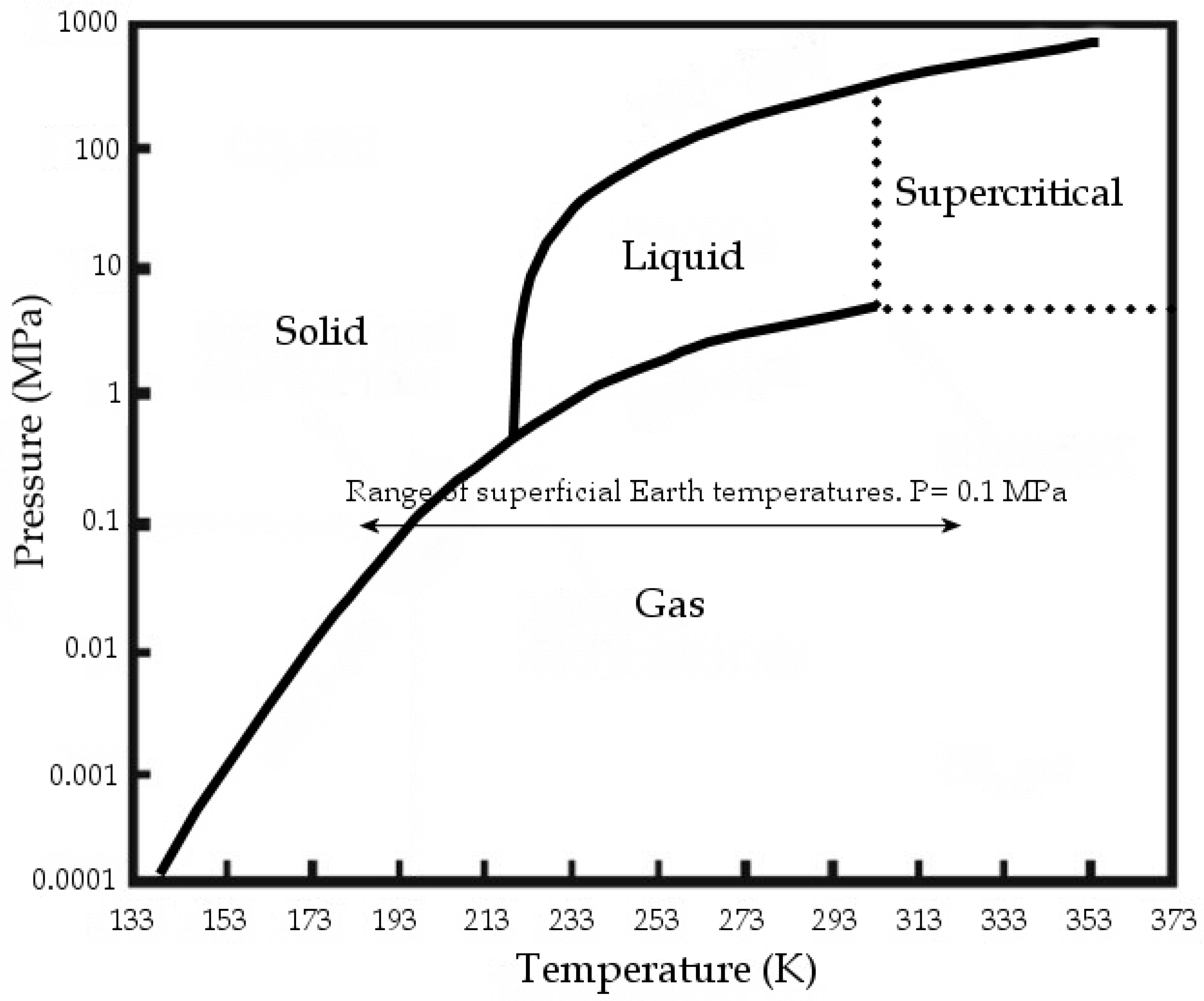
:1. Introduction
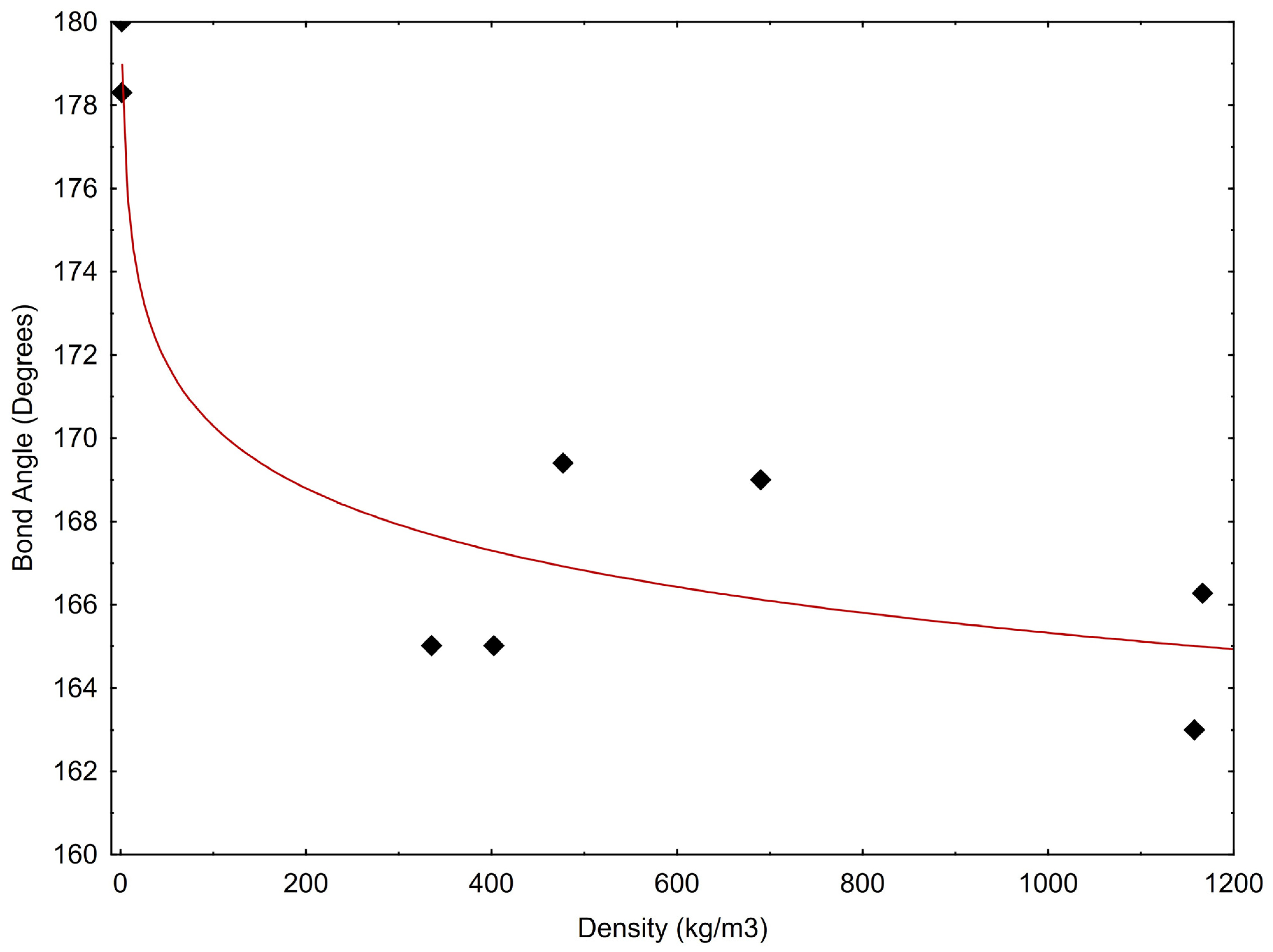
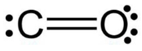
2. CO2 Molecular Structure Generalities and Geometry Variations

| Temp (K) | Press (MPa) | Density (kg/m3) | Bond Angle | Specific Enthalpy (kJ/mol) | Aggr. State According NIST | Internal Energy (kJ/mol) | Cv (J/mol·K) | Cp (J/mol·K) | Ref |
|---|---|---|---|---|---|---|---|---|---|
| 273.15 | 0.1 | 1.78 | 180 | 21.34 | 19.08 | 27.81 | 36.38 | ||
| 298 | 0.1 | 1.78 | 178.3 | 22.257 | 19.792 | 28.928 | 37.435 | [27] | |
| 220 | 0.85 | 1167 | 166.27 | 3.8198 | liq | 3.7877 | 42.696 | 86.257 | [35] |
| 320 | 10.2 | 477.4 | 169.4 | 15.659 | sc | 14.719 | 46.314 | 328.55 | [32] |
| 222 | 0.65 | 1158 | 163 | 19.027 | liq | 17.354 | 28.374 | 41.522 | [34] |
| 310 | 10.1 | 690.36 | 169 | 13.046 | sc | 12.402 | 43.801 | 190.11 | [36] |
| 320 | 9.7 | 403 | 165.01 | 16.486 | sc | 15.427 | 46.475 | 315.33 | [36] |
| 320 | 9.2 | 335.8 | 165.01 | 17.327 | sc | 16.121 | 45.272 | 240.56 | [36] |
3. A Simple Model to Evaluate the Single Molecule CO2 Dipole Moment
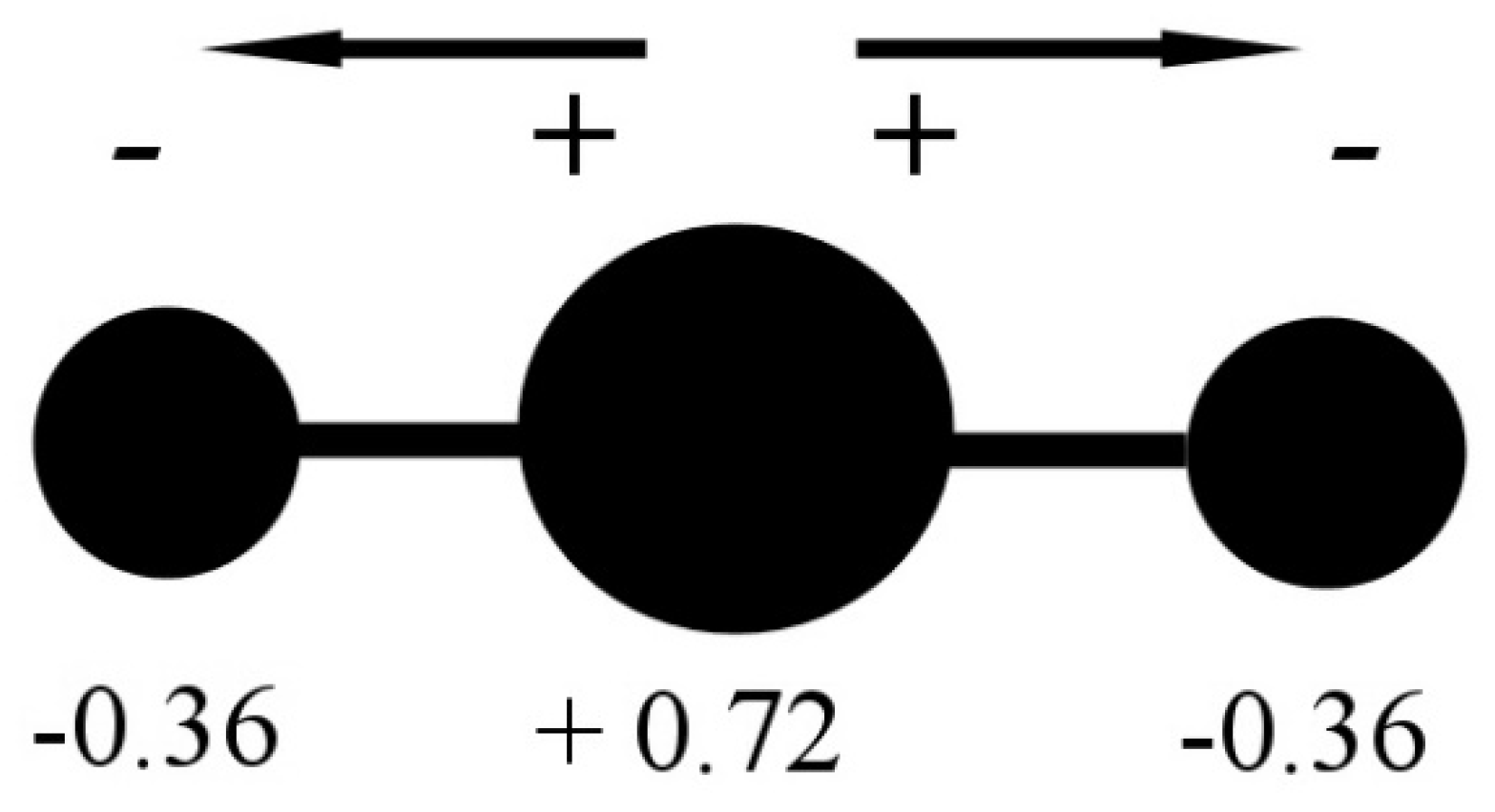
3.1. Partial Charge of Carbon and Oxygen Atoms
= 4 − [2 + 4 × (2.55/(2.55 + 3.44))] = +0.29 e;
= 6 − [4 + 4 × (3.44/(3.44 + 2.55))] = −0.29 e.
3.2. Partial Charge of the C=O Couple
3.3. The Dipole Moment of the C=O Couple
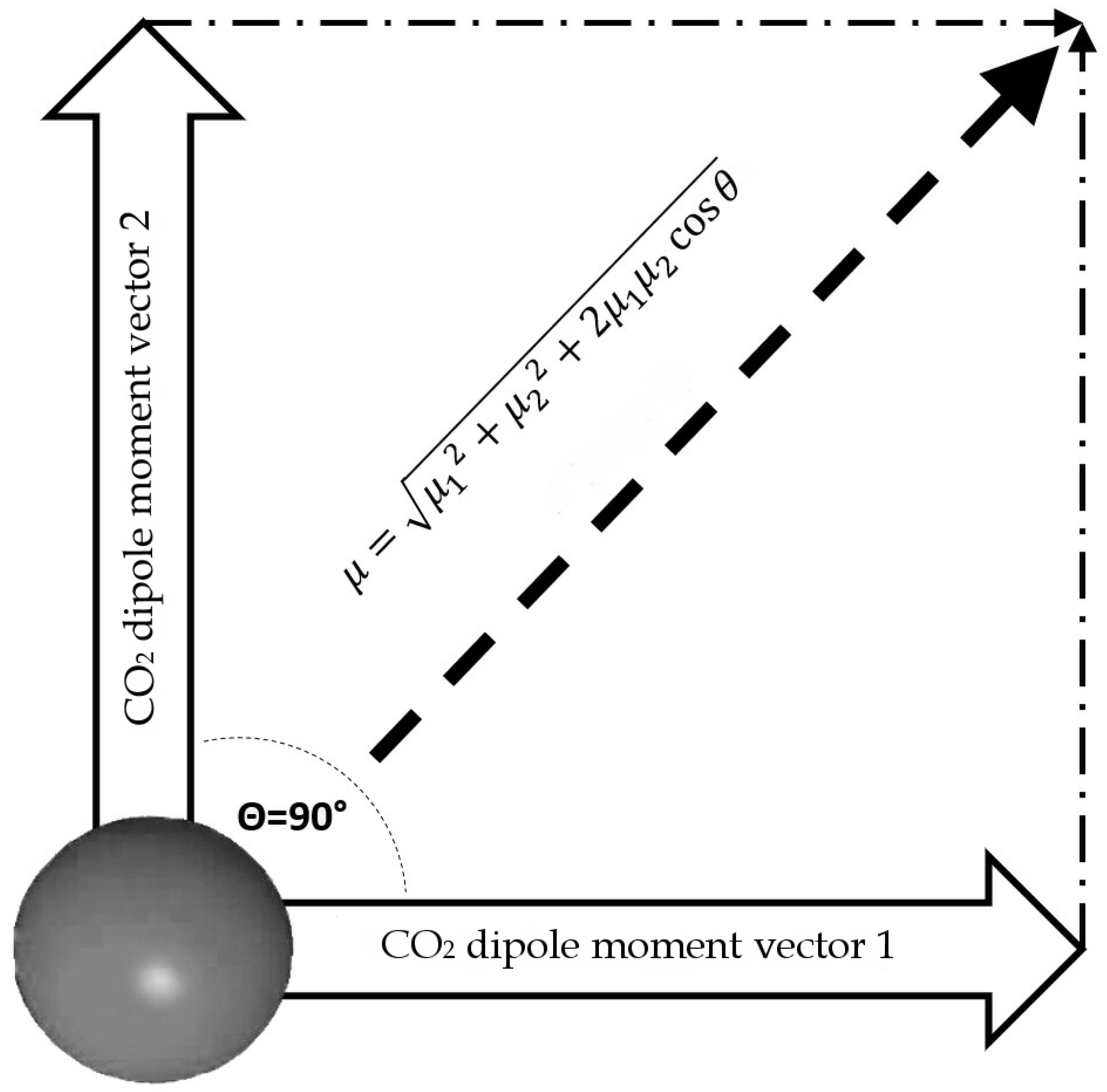
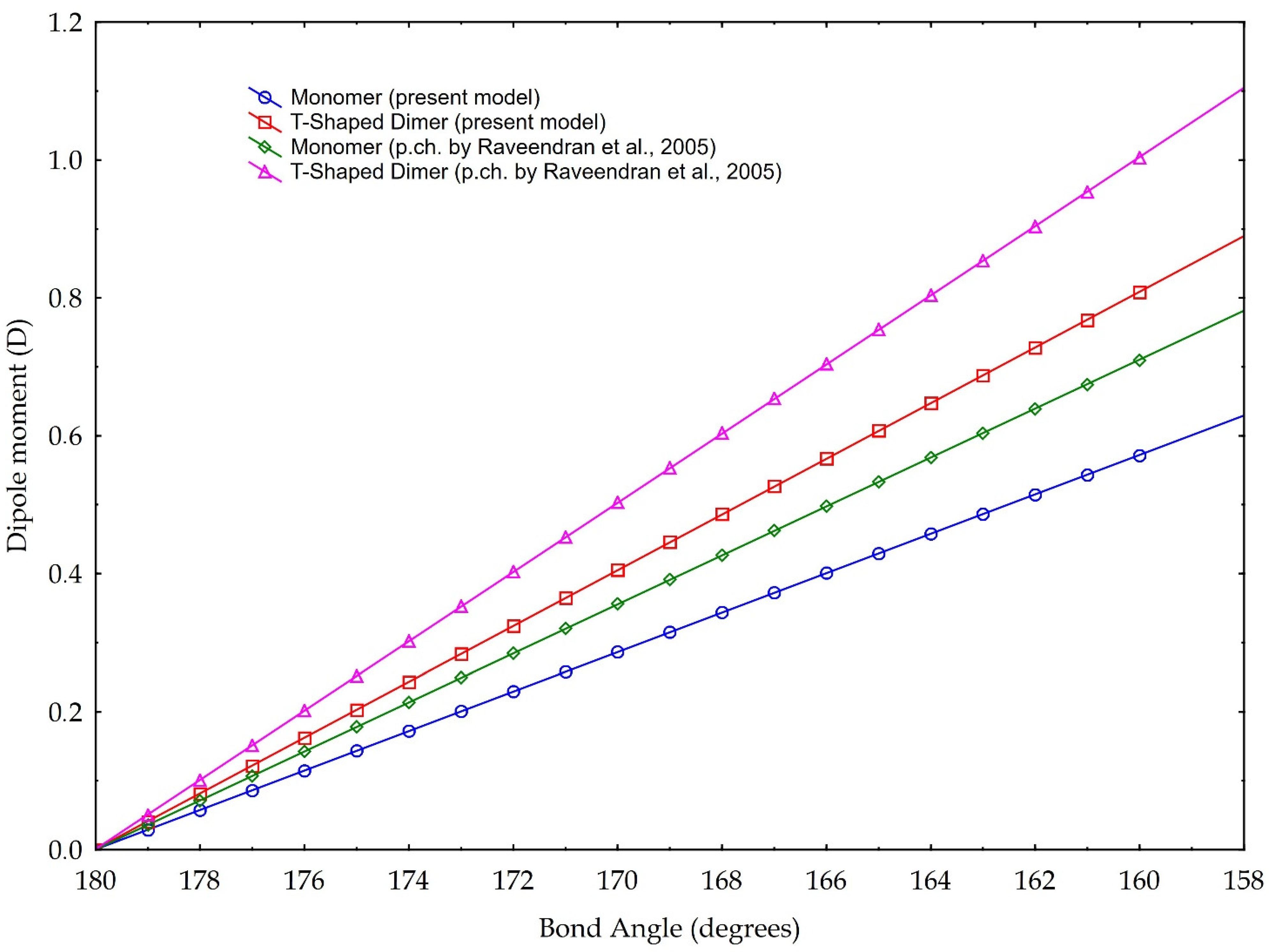
3.4. The Dipole Moment of the Entire CO2 Molecule
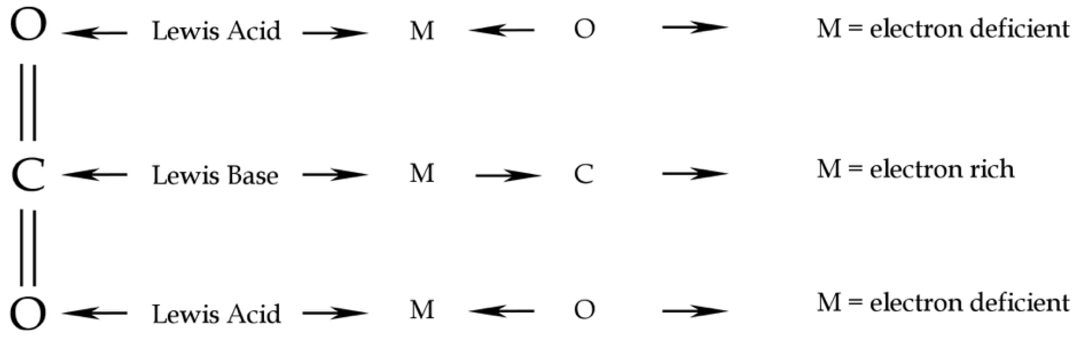
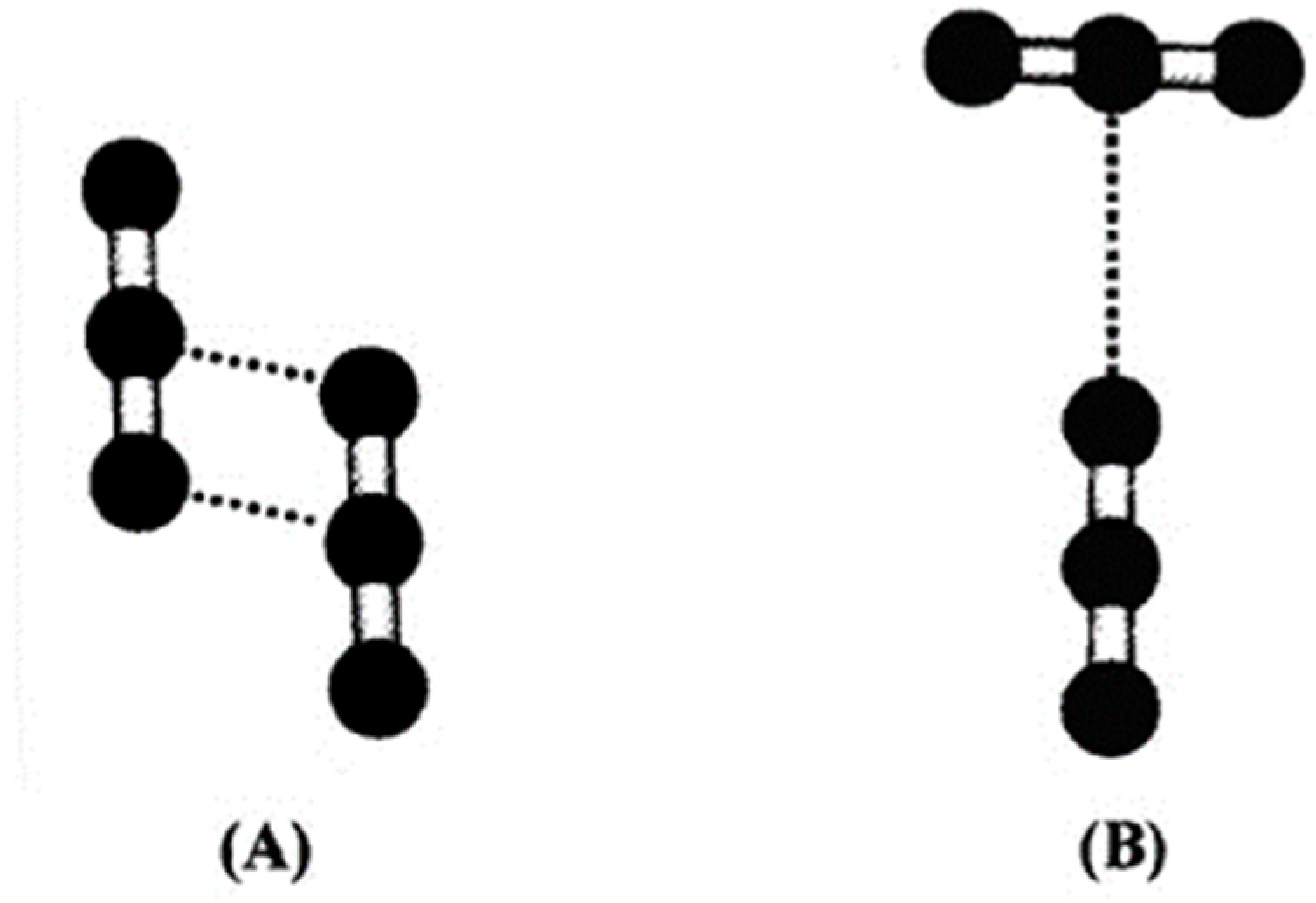
4. Discussion
Capability of CO2 to Bind and Solubilise Elements
5. Conclusions
Author Contributions
Funding
Data Availability Statement
Acknowledgments
Conflicts of Interest
References
- Witowski, A.; Majkut, M.; Rulik, S. Analysis of pipeline transportation systems for carbon dioxide sequestration. Arch. Thermodyn. 2014, 35, 117–140. [Google Scholar] [CrossRef] [Green Version]
- Buckingham, A.D.; Disch, R.L. The Quadrupole Moment of the Carbon Dioxide Molecule. Proc. R. Soc. Lond. Ser. A Math. Phys. Sci. 1963, 273, 275–289. [Google Scholar] [CrossRef]
- Raveendran, P.; Ikushima, Y.; Wallen, S.L. Polar Attributes of Supercritical Carbon Dioxide. Acc. Chem. Res. 2005, 38, 478–485. [Google Scholar] [CrossRef] [PubMed]
- Raveendran, P.; Wallen, S.L. Cooperative C-H···O Hydrogen Bonding in CO2-Lewis Base Complexes: Implications for Solvation in Supercritical CO2. J. Am. Chem. Soc. 2002, 124, 12590–12599. [Google Scholar] [CrossRef]
- Sahena, F.; Zaidul, I.S.M.; Jinap, S.; Karim, A.A.; Abbas, K.A.; Norulaini, N.A.N.; Omar, A.K.M. Application of supercritical CO2 in lipid extraction—A review. J. Food Eng. 2009, 95, 240–253. [Google Scholar] [CrossRef]
- Gouveia, L.; Nobre, B.P.; Marcelo, F.M.; Mrejen, S.; Cardoso, M.T.; Palavra, A.F.; Mendes, R.L. Functional food oil coloured by pigments extracted from microalgae with supercritical CO2. Food Chem. 2007, 101, 717–723. [Google Scholar] [CrossRef]
- De Marco, I.; Riemma, S.; Iannone, R. Life cycle assessment of supercritical CO2 extraction of caffeine from coffee beans. J. Supercrit. Fluids 2018, 133, 393–400. [Google Scholar] [CrossRef]
- Subramaniam, B.; Rajewski, R.A.; Snavely, K. Pharmaceutical processing with supercritical carbon dioxide. J. Pharm. Sci. 1997, 86, 885–890. [Google Scholar] [CrossRef]
- Bertucco, A.; Canu, P.; Devetta, L.; Zwahlen, A.G. Catalytic Hydrogenation in Supercritical CO2: Kinetic Measurements in a Gradientless Internal-Recycle Reactor. Ind. Eng. Chem. Res. 1997, 36, 2626–2633. [Google Scholar] [CrossRef]
- Blanchard, L.A.; Gu, Z.; Brennecke, J.F. High-Pressure Phase Behavior of Ionic Liquid/CO2 Systems. J. Phys. Chem. B 2001, 105, 2437–2444. [Google Scholar] [CrossRef]
- Rochelle, C.A.; Moore, Y.A. The Solubility of Supercritical CO2 into Pure Water and Synthetic Utsira Porewater; British Geological Survey: Nottingham, UK, 2002; 28p. [Google Scholar]
- Wang, Z.; Zhou, Q.; Guo, H.; Yang, P.; Lu, W. Determination of water solubility in supercritical CO2 from 313.15 to 473.15 K and from 10 to 50 MPa by in-situ quantitative Raman spectroscopy. Fluid Phase Equilibria 2018, 476, 170–178. [Google Scholar] [CrossRef]
- Regnault, O.; Lagneau, V.; Catalette, H.; Schneider, H. Étude expérimentale de la réactivité du CO2 supercritique vis-à-vis de phases minérales pures. Implications pour la séquestration géologique de CO2. C. R. Geosci. 2005, 337, 1331–1339. [Google Scholar] [CrossRef]
- Regnault, O.; Lagneau, V.; Schneider, H. Experimental measurement of portlandite carbonation kinetics with supercritical CO2. Chem. Geol. 2009, 265, 113–121. [Google Scholar] [CrossRef]
- Criscenti, L.J.; Cygan, R.T. Molecular Simulations of Carbon Dioxide and Water: Cation Solvation. Environ. Sci. Technol. 2013, 47, 87–94. [Google Scholar] [CrossRef]
- Rempel, K.U.; Liebscher, A.; Heinrich, W.; Schettler, G. An experimental investigation of trace element dissolution in carbon dioxide: Applications to the geological storage of CO2. Chem. Geol. 2011, 289, 224–234. [Google Scholar] [CrossRef]
- Di Noto, V.; Vezzù, K.; Conti, F.; Giffin, G.A.; Lavina, S.; Bertucco, A. Broadband Electric Spectroscopy at High CO2 Pressure: Dipole Moment of CO2 and Relaxation Phenomena of the CO2–Poly(vinyl chloride) System. J. Phys. Chem. B 2011, 115, 9014–9021. [Google Scholar] [CrossRef]
- Santosh, M.; Omori, S. CO2 flushing: A plate tectonic perspective. Gondwana Res. 2008, 13, 86–102. [Google Scholar] [CrossRef]
- Stewart, E.M.; Ague, J.J.; Ferry, J.M.; Schiffries, C.M.; Tao, R.B.; Terry, T.; Isson, T.T.; Noah, J.; Planavsky, N.J. Carbonation and decarbonation reactions: Implications for planetary habitability. Am. Mineral. 2019, 104, 1369–1380. [Google Scholar] [CrossRef] [Green Version]
- Gibbins, J.; Chalmers, H. Carbon capture and storage. Energy Policy 2000, 36, 4317–4322. [Google Scholar] [CrossRef] [Green Version]
- Zhang, M.; Zhan, S.; Jin, Z. Recovery mechanisms of hydrocarbon mixtures in organic and inorganic nanopores during pressure drawdown and CO2 injection from molecular perspectives. Chem. Eng. J. 2020, 382, 122808. [Google Scholar] [CrossRef]
- Pruess, K. On production behavior of enhanced geothermal systems with CO2 as working fluid. Energy Convers. Manag. 2008, 49, 1446–1454. [Google Scholar] [CrossRef] [Green Version]
- Borgia, A.; Pruess, K.; Kneafsey, T.J.; Oldenburg, C.M.; Pan, L. Simulation of CO2-EGS in a fractured reservoir with salt precipitation. Energy Procedia 2013, 37, 6617–6624. [Google Scholar] [CrossRef] [Green Version]
- Borgia, A.; Oldenburg, C.M.; Zhang, R.; Pan, L.; Daley, T.M.; Finsterle, S.; Ramakrishnan, T.S. Simulating CO2 injection into fractures and faults for Improved characterization of EGS sites. Geothermics 2017, 69, 189–201. [Google Scholar] [CrossRef] [Green Version]
- Leitner, W. The coordination chemistry of carbon dioxide and its relevance for catalysis: A critical survey. Coord. Chem. Rev. 1996, 153, 257–284. [Google Scholar] [CrossRef]
- Sato, H.; Matubayasi, N.; Nakahara, M.; Hirata, F. Which carbon oxide is more soluble? Ab initio study on carbon monoxide and dioxide in aqueous solution. Chem. Phys. Lett. 2000, 323, 257–262. [Google Scholar] [CrossRef]
- Xantheas, S.S. Ab initio studies of cyclic water clusters (H2O)n, n = 1–6. Analysis of many body interactions. J. Chem. Phys. 1994, 100, 7523. [Google Scholar] [CrossRef]
- Jena, N.R.; Mishra, P.C. An ab initio and density functional study of microsolvation of carbon dioxide in water clusters and formation carbonic acid. Theor. Chem. Acc. 2005, 114, 189–199. [Google Scholar] [CrossRef]
- Zhang, Y.; Yang, J.; Yu, Y.-X. Dielectric Constant and Density Dependence of the Structure of Supercritical Carbon Dioxide Using a New Modified Empirical Potential Model: A Monte Carlo Simulation. J. Phys. Chem. B 2005, 109, 13375–13382. [Google Scholar] [CrossRef]
- Cipriani, P.; Nardone, M.; Ricci, F.P.; Ricci, M.A. Orientational correlations in liquid and supercritical CO2: Neutron diffraction experiments and molecular dynamics simulations. Mol. Phys. 2001, 99, 301–308. [Google Scholar] [CrossRef]
- Saharay, M.; Balasubramanian, S. Enhanced Molecular Multipole Moments and Solvent Structure in Supercritical Carbon Dioxide. ChemPhysChem 2004, 5, 1442–1445. [Google Scholar] [CrossRef]
- Mi, W.; Ramos, P.; Maranhao, J.; Pavanello, M. Ab Initio Structure and Dynamics of CO2 at Supercritical Conditions. J. Phys. Chem. Lett. 2019, 10, 7554–7559. [Google Scholar] [CrossRef] [PubMed]
- Saharay, M.; Balasubramanian, S. Evolution of Intermolecular Structure and Dynamics in Supercritical Carbon Dioxide with Pressure: An ab Initio Molecular Dynamics Study. J. Phys. Chem. B 2007, 111, 387–392. [Google Scholar] [CrossRef] [PubMed]
- Anderson, K.E.; Mielke, S.L.; Siepmann, J.I.; Donald, G.; Truhlar, D.G. Bond Angle Distributions of Carbon Dioxide in the Gas, Supercritical, and Solid Phases. J. Phys. Chem. A 2009, 113, 2053–2059. [Google Scholar] [CrossRef] [PubMed]
- Adya, A.K.; Wormald, C.J. Intra and intermolecular structure in the condensed phases of ethylene, ethane and carbon dioxide by neutron diffraction. Mol. Phys. 1992, 77, 1217–1246. [Google Scholar] [CrossRef]
- Ishii, R.; Okazaki, S.; Odawara, O.; Okada, I.; Misawa, M.; Fukunaga, T. Structural study of supercritical carbon dioxide by neutron diffraction. Fluid Phase Equilibria 1995, 104, 291–304. [Google Scholar] [CrossRef]
- Silvestroni, P. Fondamenti di Chimica; College English Association: San Antonio, TX, USA, 1996; ISBN 8808084019. [Google Scholar]
- Wilmshurst, J.K. An Empirical Expression for Bond Dipole Moments. J. Phys. Chem. 1958, 62, 631–633. [Google Scholar] [CrossRef]
- Breneman, C.M.; Wiberg, K.B. Determining atom-centered monopoles from molecular electrostatic potentials. The need for high sampling density in formamide conformational analysis. J. Comp. Chem. 1990, 11, 361. [Google Scholar] [CrossRef]
- Schaef, H.T.; Loganathan, N.; Bowers, G.M.; Kirkpatrick, R.J.; Yazaydin, A.O.; Burton, S.D.; Hoyt, D.W.; Thanthiriwatte, K.S.; Dixon, D.A.; McGrail, B.P.; et al. Tipping Point for Expansion of Layered Aluminosilicates in Weakly Polar Solvents: Supercritical CO2. ACS Appl. Mater. Interfaces 2017, 9, 36783–36791. [Google Scholar] [CrossRef] [Green Version]
- Propp, W.A.; Carleson, T.E.; Wai, C.M.; Huang, S. Transport of Metal Sulfides in Supercritical Carbon Dioxide; Lockheed Idaho Technologies Co.: Idaho Falls, CO, USA, 1996. [Google Scholar] [CrossRef] [Green Version]
- Sanguinito, S.; Goodman, A.; Tkach, M.; Kutchko, B.; Culp, J.; Natesakhawat, S.; Fazio, J.; Fukai, I.; Crandall, D. Quantifying dry supercritical CO2-induced changes of the Utica Shale. Fuel 2018, 226, 54–64. [Google Scholar] [CrossRef]
- Kwak, J.H.; Hu, J.Z.; Turcu, R.V.F.; Rosso, K.M.; Ilton, E.S.; Wang, C.; Sears, J.A.; Engelhard, M.H.; Felmy, A.R.; David, W.; et al. The role of H2O in the carbonation of forsterite in supercritical CO2. Int. J. Greenh. Gas Control. 2011, 5, 1081–1092. [Google Scholar] [CrossRef]
- Rahmani, O.; Highfield, J.; Junin, R.; Tyrer, M.; Pour, A.B. Experimental Investigation and Simplistic Geochemical Modeling of CO₂ Mineral Carbonation Using the Mount Tawai Peridotite. Molecules 2016, 21, 353. [Google Scholar] [CrossRef] [Green Version]
- Sugama, T.; Ecker, L.; Butcher, T. Carbonation of Rock Minerals by Supercritical Carbon Dioxide at 250 °C; Energy Resources Department/Energy Resources Division Brookhaven National Laboratory: Upton, LI, USA, 2010; p. 25. [Google Scholar] [CrossRef] [Green Version]
- Tutolo, B.M.; Luhmann, A.J.; Kong, X.Z.; Saar, M.O.; Seyfried, W.E., Jr. Experimental Observation of Permeability Changes In Dolomite at CO2 Sequestration Conditions. Environ. Sci. Technol. 2014, 48, 2445–2452. [Google Scholar] [CrossRef]
- Xu, T.; Pruess, K.; Apps, J. Numerical Studies of Fluid Rock Interaction in Enhanced Geothermal Systems (EGS) with CO2 as Working Fluid. In Proceedings of the Thirty-Third Workshop on Geothermal Reservoir Engineering Stanford University, Stanford, CA, USA, 28–30 January 2008. [Google Scholar]
- Lupton, J.; Butterfield, D.; Lilley, M.; Evans, L.; Nakamura, K.; Chadwick Jr., W.; Resing, J.; Embley, R.; Olson, E.; Proskurowski, G.; et al. Submarine venting of liquid carbon dioxide on a Mariana Arc volcano. Geochem. Geophys. Geosyst. 2006, 7, Q08007. [Google Scholar] [CrossRef] [Green Version]
- Chivas, A.R.; Barnes, I.; Evans, W.C.; Lupton, J.E.; Stone, J.O. Liquid carbon dioxide of magmatic origin and its role in volcanic eruptions. Nature 1987, 326, 587–589. [Google Scholar] [CrossRef]
- Beccaluva, L.; Bonatti, E.; Dupuy, C.; Ferrara, G.; Innocenti, F.; Lucchini, F.; Macera, P.; Petrini, R.; Rossi, P.L.; Serri, G.; et al. Geochemistry and Mineralogy of Volcanic Rocks from ODP Sites 650, 651, 655, and 654 in the Tyrrhenian Sea. Proc. Ocean. Drill. Program Sci. Results 1990, 107, 49–74. [Google Scholar] [CrossRef]
- Lauro, S.E.; Pettinelli, E.; Caprarelli, G.; Guallini, L.; Rossi, A.P.; Mattei, E.; Cosciotti, B.; Cicchetti, A.; Soldovieri, F.; Cartacci, M.; et al. Multiple subglacial water bodies below the south pole of Mars unveiled by new MARSIS data. Nat. Astron. 2020, 5, 63–70. [Google Scholar] [CrossRef]
- Booth, M.C.; Kieffer, H.H. Carbonate formation in Marslike environments. J. Geophys. Res. 1978, 83, 1809–1815. [Google Scholar] [CrossRef]
- Stephens, S.K.; Stevenson, D.J. Dry Carbonate Formation on Mars: A Plausible Sink for an Early Dense CO2 Atmosphere? In Proceedings of the Lunar and Planetary Science Conference, Houston, TX, USA, 12–18 March 1990; Volume 21, p. 56. [Google Scholar]
- Wray, J.J.; Murchie, S.L.; Bishop, J.L.; Ehlmann, B.L.; Milliken, R.E.; Wilhelm, M.B.; Seelos, K.D.; Chojnacki, M. Orbital evidence for more widespread carbonate-bearing rocks on Mars. J. Geophys. Res. Planets 2016, 121, 652–677. [Google Scholar] [CrossRef]
- Di Lorenzo, F.; Ruiz-Agudo, C.; Ibañez-Velasco, A.; Gil-San Millán, R.; Navarro, J.A.R.; Ruiz-Agudo, E.; Rodriguez-Navarro, C. The Carbonation of Wollastonite: A Model Reaction to Test Natural and Biomimetic Catalysts for Enhanced CO2 Sequestration. Minerals 2018, 8, 209. [Google Scholar] [CrossRef] [Green Version]
- Kelektsoglou, K. Carbon Capture and Storage: A Review of Mineral Storage of CO2 in Greece. Sustainability 2018, 10, 4400. [Google Scholar] [CrossRef]


| Temp (K) | Press (Mpa) | Density (kg/m3) | Bond Angle | Specific Enthalpy (kJ/mol) | Internal Energy (kJ/mol) | Cv (J/mol·K) | Cp (J/mol·K) | |
|---|---|---|---|---|---|---|---|---|
| Temp (K) | 1.00 | 0.77 | −0.67 | 0.15 | 0.34 | 0.38 | 0.50 | 0.72 |
| Press (Mpa) | 0.77 | 1.00 | −0.07 | −0.43 | −0.14 | -0.08 | 0.85 | 0.94 |
| Density (kg/m3) | -0.67 | -0.07 | 1.00 | −0.74 | -0.69 | -0.69 | 0.19 | -0.08 |
| Bond Angle | 0.15 | −0.43 | −0.74 | 1.00 | 0.48 | 0.45 | −0.56 | −0.44 |
| Specific Enthalpy (kJ/mol) | 0.34 | −0.14 | −0.69 | 0.48 | 1.00 | 1.00 | −0.58 | −0.17 |
| Internal energy (kJ/mol) | 0.38 | −0.084 | −0.69 | 0.45 | 1.00 | 1.00 | −0.54 | −0.12 |
| Cv (J/mol·K) | 0.50 | 0.85 | 0.19 | −0.56 | −0.58 | −0.54 | 1.00 | 0.88 |
| Cp (J/mol·K) | 0.72 | 0.94 | −0.08 | −0.44 | −0.17 | −0.12 | 0.88 | 1.00 |
| Factor 1 | Factor 2 | |
|---|---|---|
| Temp (K) | −0.53 | 0.83 |
| Press (Mpa) | 0.07 | 0.97 |
| Density (kg/m3) | 0.91 | −0.19 |
| Bond Angle | −0.72 | −0.35 |
| Specific Enthalpy (kJ/mol) | −0.92 | −0.11 |
| Internal energy (kJ/mol) | −0.91 | −0.06 |
| Cv (J/mol·K) | 0.46 | 0.87 |
| Cp (J/mol·K) | 0.1 | 0.97 |
| % Total Variance | 48.53 | 39.41 |
| Cumulative Variance | 48.53 | 87.94 |
| Eigenvalue | 3.88 | 3.15 |
| Cumulative Eigenvalue | 3.88 | 7.03 |
| Number (n) of Water Molecules | Dipole Moment (Debye) |
|---|---|
| 3 | 0.837 |
| 4 | 2.325 |
| 5 | 4.192 |
| 6 | 1.235 |
| 7 | 4.419 |
| 8 | 3.400 |
| Extraction (mg Metal/g Fluid) | ||||||||
|---|---|---|---|---|---|---|---|---|
| Fluid | As | Cd | Co | Cu | Pb | Fe | Ni | Zn |
| Pure CO2 0.76 g/mL, 71 °C | 7.6 × 10⁻⁴ | 1.8 × 10⁻⁵ | 1.1 × 10⁻⁵ | 1.0 × 10⁻³ | 2.8 × 10⁻⁴ | 4.2 × 10⁻⁴ | 1.3 × 10⁻² | 4.7 × 10⁻³ |
| Water 0.99 g/mL, 68 °C | 2.4 × 10⁻² | 1.5 × 10⁻⁴ | 2.2 × 10⁻⁴ | 6.2 × 10⁻⁵ | 2.0 × 10⁻⁵ | 1.2 × 10⁻² | 3.2 × 10⁻⁴ | 1.2 × 10⁻⁴ |
Disclaimer/Publisher’s Note: The statements, opinions and data contained in all publications are solely those of the individual author(s) and contributor(s) and not of MDPI and/or the editor(s). MDPI and/or the editor(s) disclaim responsibility for any injury to people or property resulting from any ideas, methods, instructions or products referred to in the content. |
© 2023 by the authors. Licensee MDPI, Basel, Switzerland. This article is an open access article distributed under the terms and conditions of the Creative Commons Attribution (CC BY) license (https://creativecommons.org/licenses/by/4.0/).
Share and Cite
Calcara, M.; Caricaterra, M. CO2 Dipole Moment: A Simple Model and Its Implications for CO2-Rock Interactions. Minerals 2023, 13, 87. https://doi.org/10.3390/min13010087
Calcara M, Caricaterra M. CO2 Dipole Moment: A Simple Model and Its Implications for CO2-Rock Interactions. Minerals. 2023; 13(1):87. https://doi.org/10.3390/min13010087
Chicago/Turabian StyleCalcara, Massimo, and Matteo Caricaterra. 2023. "CO2 Dipole Moment: A Simple Model and Its Implications for CO2-Rock Interactions" Minerals 13, no. 1: 87. https://doi.org/10.3390/min13010087