CO₂ Reaction-Diffusion Experiments in Shales and Carbonates

Abstract

The evaluation of caprock integrity and reservoir efficiency is critical for safe CO₂ geological storage management. It is therefore important to investigate geochemical reactions between CO₂-rich fluids and host rocks and their contribution in retaining CO₂ at depth. This study deals with diffusive reaction experiments on shales and carbonate samples cored from an offshore structure in the Malaysian basin, a potential target for CO₂-enhanced gas recovery. The aim is to evaluate the CO₂ reaction front velocity in a typical shaly caprock and the mineral response of the reservoir. Rock samples were characterized in terms of texture, chemistry, and mineralogy by X-ray diffraction, electron microscopy (SEM), microanalysis (EDS), infrared spectroscopy (FT-IR), rock geochemistry (XRF), and mercury injection capillary permeability (MICP). Performed analyses show mineralogical alteration induced by CO₂ as it penetrated into the samples. Carbonate dissolution and weathering of pyrite to form secondary carbonates belonging to siderite-ankerite series were observed along two reaction fronts. Estimated diffusion coefficients of CO₂ are two orders of magnitude lower than CO_2(aq) molecular diffusion in pure water and from half to an order of magnitude lower than diffusivity computed on unaltered sample, highlighting the important effect of gas–water–rock reactions on the CO_2(aq) diffusivities in shales and carbonates. Results obtained in this study provide an insight regarding the effect of geochemical reactions on CO₂ transport and represent a further discussion point on the diffusion coefficients.

1. Introduction

CO₂ geological storage (CCS) has been recognized as able to efficiently mitigate the climate change induced by greenhouse gasses [1,2,3,4]. In order to ensure a safe storage of CO₂ at depth, potential leakage from the reservoir throughout the overburden have to be carefully evaluated [5,6,7,8,9].

In sedimentary basins, shales are generally considered optimal caprock for CCS reservoirs since they are characterized by low permeability and high capillary entry pressure which prevent migration of injected CO₂ toward the surface. In addition, they are mainly constituted by siliciclastic and clay minerals, which can react with CO₂-rich brines, permanently trapping CO₂ as newly formed solid phases [10]. These solid phases are generally present also in sandstones and limestones reservoirs, although in minor amounts. The dissolution of primary minerals and the precipitation of secondary ones control the porosity and the permeability of the hosting rock, ruling the velocity of the CO₂ reaction front at the caprock–reservoir interface. Depending on mineral assemblage, fluid chemical composition, and boundary conditions, geochemical reactions may contribute to retain CO₂ at depth by self-sealing process or to enhance fluid migration towards the surface by mineral dissolution; and they should be evaluated throughout site-specific analyses.

The characterization of rocks mineralogical and petrophysical alteration due to CO₂ injection can be carried out by laboratory analysis and experiments at in-situ condition by using available, site-specific rock samples [11,12,13]. Due to the slow kinetics of some minerals (e.g., siliciclastic and clayey), laboratory experiments allow to evaluate the chemical weathering effect on reservoir and caprock stability only in the short-term, but they can be a useful tool to obtain reliable geochemical input parameters for long-term numerical models, covering uncertainties linked to kinetic rates, mineral reactive surface areas, petrophysical properties of rocks, and diffusion coefficients of supercritical CO₂.

In this framework, the objective of this study is to qualitatively evaluate the geochemical reactions induced by CO₂ in a carbonate reservoir and on the shaly caprock and quantify the velocity of reaction front by means of reaction-diffusion experiments. A depleted hydrocarbon reservoir, in offshore Malaysia, a potential target for CO₂ geological storage [14], was used as a case study for our experiments, focusing on shale overburden, which is often neglected during hydrocarbon exploitation.

The texture, geochemistry, and mineral composition of three selected rock samples were determined before and after alteration experiments, combining several petrophysical techniques: X-ray diffraction, rock geochemistry (XRF), electron microscopy plus energy dispersive system (SEM-EDS), infrared spectroscopy (FT-IR), and mercury injection capillary permeability (MICP).

The lab analysis and diffusion experiments allowed to: (i) characterize the mineralogy of cores; (ii) describe their changes related to geochemical weathering induced by CO₂; (iii) evaluate the velocity of CO₂ penetration into the samples; and (iv) estimate the CO₂ diffusion coefficients. Following our previous methodological approach (e.g., [15]), these results provide information to set and calibrate reliable reactive transport models useful to investigate short-to-long-term consequences of CO₂ storage and to evaluate the effect of trapping mechanisms on fluid flow [16].

2. Materials and Methods

2.1. Geological Structure, Rock Formations and Studied Samples

The selected study structure (Figure 1a) is located in the north of Central Luconia Province in the Sarawak Basin, East Malaysia. Sedimentary stratigraphy of the area can be divided in 8 regressive cycles (from the Eocene to present) that are separated by major transgressions [17,18]. In the selected structure, rock formations belong to V-VII sedimentary cycles [19], which are comprised of middle Miocene carbonate reservoir (V cycle) discordantly overlain by Pliocene sediments (VI and VII cycles). The overburden formations are thick, approximately 2000 m, and consist mainly of interbedded silt, silty clay, and shale intervals. They are divided in three main layers based on the contrast in sonic-log velocity: soft sediments right below the seabed, the Seal 6 and below the Seal 4 (Figure 1a). Based on the quick correlation, the presence of silty layers is prominent in Seal 6 while shales dominate Seal 4 with some intercalation of silt. The underlying reservoir is constituted by fractured limestones. Geothermal and geobaric gradients (Figure 1b), measured in well logs, show a high-temperature, high-pressure zone from around 1400 m of depth, roughly corresponding to Seal4 top to the reservoir (133 °C and 315 bar at about 1900 m, top reservoir).

Rock samples employed in diffusion experiments were taken from a deep well, located in the case study structure and provided by operator. Generally speaking, in hydrocarbon exploration very limited attention is reserved for coverture characterization, mainly focusing on the reservoir. Only three rocks samples (C1, C2, and C3), representing Seal 6, Seal 4, and limestone reservoir matrix (Figure 1a), were available for the experiments.

2.2. Sample Preparation and Characterization

Petrophysical analysis of cores was performed before and after the alteration experiments to study textural and mineralogical changes.

In particular, X-ray diffraction (XRPD), X-ray fluorescence (XRF), Rietveld, and electron with energy dispersive system microscopy (SEM-EDS) (Carl Zeiss, Oberkochen, Germany) analyses were carried out before the diffusion experiments to define chemical composition of the samples and semi-quantitative and morphological evaluation of minerals. SEM-EDS analyses were repeated after experiments to evaluate the alteration degree and the velocity of the reaction front. Infrared spectroscopy (FT-IR) (is50, Thermo Fisher Scientific Inc., Waltham, MA, USA) was used to further evaluate the compositional changes, allowing an easy comparison among spectra of pristine and altered materials. Finally, mercury injection capillary pressure (MICP) analyses were also carried out to measure porosity, pore distribution, and tortuosity.

All original samples were massive and well-preserved. After experiments, shale specimens were still cohesive, but after the SEM analyses, preparation, and storage, they progressively lost cohesion (Figure 1d,e), requiring different analytical procedures as described below.

Before starting diffusion experiments, each rock was cut to obtain a representative sample and heated in an oven for five days at 40 °C to avoid a crumbly braking of clays and remove the water present in the samples. This procedure is necessary to evaluate the weight of the sample at dry and saturated conditions before and after the experiments.

A rock portion of initial cores was powdered for XRPD and XRF analysis, whereas another one was cut to create a thin section for SEM-EDS analysis. Finally, a core fraction was devoted to destructive analysis of MICP.

The XRPD analyses were performed on powdered samples by using an X-ray Philips PW 1050/37 diffractometer (PW 1050/37, Philips, Amsterdam, Netherlands), with the X’Pert PRO Philips acquisition system, operating at 40 kV-20 mA, with a Cu anode and graphite monochromator at an interval 2θ of 5–70° and 2–32° for the clay analysis. The powders were mixed with corundum at 2.5% w/w.

XRF was performed on powdered samples with a Rigaku II wavelength dispersive spectrometer (ZSX, Rikaku, Tokyo, Japan) with a Rh anode. The main composition was acquired with a ZSX Rigaku Software Package version 3.50 and quantified with the SQX semi-quantitative elemental analysis routine by the fundamental parameter (FP) method without the use of reference standard samples. In the quantifying process, a sensitivity library (Rigaku analytical system) containing the FP reference values for every element was used. Pure metals and reagents were used for the XRF calibration. The analytic error is 3% w/w for major and 10% w/w for trace elements.

CO₂ was determined as loss from carbonates by calcimetric analysis which was used to correct XRF data. The concentration of FeO was calculated by volumetric titration with Potassium dichromate (N: 0.400) (K₂Cr₂O7) on a quantity of powdered sample (up to 0.5 g), transferred to a 10 mL Pt capsule and solubilized by 10 mL of H₂SO₄ and 5 mL of HF [20] under a Bunsen burner. Natrium-diphenylamine-sulfonate (solubilized in H₂SO₄) was used as an indicator. To compute the amount of FeO (in % by weight), the mL of titration solution was multiplied for 0.4 (calibration coefficient for titrating solution).

Rietveld analyses were performed on XRPD data by Maud v2.2 code [21] to obtain the modal mineralogy. Maud v2.2 is a general diffraction/reflectivity analysis program mainly based on the Rietveld method which permits to calculate the reciprocal ratios among present phases and normalize them. Carbonate content was determined by calcimetry with a Dietrich–Fruhling apparatus, including correction for carbonates other than calcite, based on the XRPD Rietveld refinement data. XRF results for total chemical composition were then corrected including carbonate abundances.

Scanning electron microscopy equipped with an energy dispersive system (SEM/EDS) on thin sections (preliminary carbon coated) allowed rock texture and semi-quantitative chemical analysis. Morphological and morphometrical images at high resolution in a back scattered mode and micro-chemical analyses were obtained using a ZEISS EVO MA15 scanning electron microscope with microanalysis (EDS) OXFORD INCA 250 at the M.E.M.A lab. Analytical conditions include a working distance of 9mm, voltage 15–20 kV and spot size for EDS of 2 µm. Error is estimated at 5% for major elements.

After diffusion experiments SEM-EDS analyses were also performed on material positioned on stub to highlight mineralogical changes due to CO₂–water interaction. In this case, the most cohesive portion of C1 and C2 specimens was taken carefully considering the orientation with respect to the fluid interaction front during the experiment.

FT-IR analyses were carried out by a Nicolet is50 instrument equipped with a Polaris™ long-life IR source (is50, Thermo Fisher Scientific Inc., Waltham, MA, USA). Spectra were acquired in the 7400–400 cm⁻¹ range on grain fraction taken from the original samples and from the altered zone after the experiments. Furthermore, the original C3 and C1 samples and C3 altered sample allowed analysis as blocks in NIR mode. For the NIR range, sample portions and blocks were positioned on a glass lamina and analyzed in the Integrating Sphere module using a InGaAs detector and a CaF₂ beamsplitter; settings included 8 resolution, 1 sample gain, 70 aperture. The rest of spectrum range was acquired on grain portions pressed under a built-in mid- and far-IR capable diamond ATR using the DTGS detector and the KBr beamsplitter; settings included 4 resolution, 1 sample gain, 100 aperture. Hence, 50 scans were acquired in both cases. An air dryer fluxing air up to 34 l/m at the dew point of –75 °C and low (down to 1 ppm) CO₂ was used to purge the system. The OMNIC Data Collector 9.11© provided instrument control, data acquisition, and spectra elaboration.

Finally, porosity, pore distribution, and tortuosity were determined by MICP on 1 cm³ specimens from original samples, after drying to 105 °C. Thermo Scientific™ Pascal Mercury Porosimeter (PASCAL 120 and 240) instruments (PASCAL 120 and 240, Thermo Fisher Scientific Inc., Waltham, MA, USA) were used to determine macropores (with diameter ranging from 116 to 3.8 µm) and micropores (from 15 to 0.0074 µm) working up the maximum pressure of 200 MPa and temperature of 22 °C. The samples were first submitted to a vacuum to degas the material and to permit the mercury filling of the dilatometer. The PASCAL instruments were managed by the S.O.L.I.D. (SOLver of Intrusion Data) software (by Thermo Fisher Scientific) to elaborate raw data.

2.3. Experimental Settings

The diffusion experiments allow to define the velocity of reactive reaction front in a rock by placing a solution with high concentration of CO₂ in contact with an intact rock for a certain period of time; in this study, for 2–5 days.

Experiment duration was calibrated based for both the small dimension of the specimens and estimated velocity of the diffusion front, to allow a noticeable CO₂ diffusion (some mm) while leaving an unaltered core zone, to be able to detect the altered/unaltered boundary. In this short period of time, only fast kinetic reactions (i.e., carbonate, oxides and pyrite) and clay mineral structure changes were expected to occur after weathering, since clay minerals take within weeks to months to fully react [22].

Original carbonate reservoir sample (C3) was cut in two cubes of 1 × 1 × 1 cm each and positioned on the base of the micro-reactor (Figure 2). In this way, the reaction with CO₂-rich brine proceeds symmetrically from the external to internal of the cube by means of diffusion only. Shale samples of Seal 6 and Seal 4 (C1 and C2, respectively), due to the clay swelling and sample dissolution in water, were cut in cylinders of about 1 × 3 cm and inserted in a custom-made reaction vessel in high density polytetrafluoroethylene (PTFE) open from two sides to allow the reaction.

The experimental apparatus is a micro-reactor 4590 HP/HT (manufactured by Parr Instrument Company, Moline, IL, USA), equipped with perfluoroelastomer (FFKM) O-ring for temperatures up to 300 °C, 200 bar. In each experiment, the micro-reactor was charged with one specimen and 5.5 mL of MilliQ water (enough to completely submerge the sample). The micro-reactor was initially flushed with pure CO_2(g) to get rid of atmospheric air before setting the CO₂ partial pressure (PCO₂). The specimen within the micro-reactor was completely immersed in water and covered by a thin layer of water, separating the gas phase, above, from the rock below (Figure 2). This thin water layer is crossed by a diffusive CO₂ flux controlling reaction front.

Experiments were carried out at temperatures of 75 °C, 105 °C and 145 °C, corresponding to Seal 6 (C1), Seal 4 (C2), and reservoir (C3) core samples at in-situ conditions (Figure 1b) and PCO₂ of 60 bars. Experimental pressure, employed for all the experiments, was subject to CO₂ cylinder availability, a maximum pressure of 60 bars.

After experiments, the samples were taken out from the apparatus, dried in a 40 °C oven to recover mechanical consistency of the material, extracted from the reaction vessel, and weighted again. The specimens were then cut in half, from the CO₂-rich brine exposed side toward the inner part.

3. Results

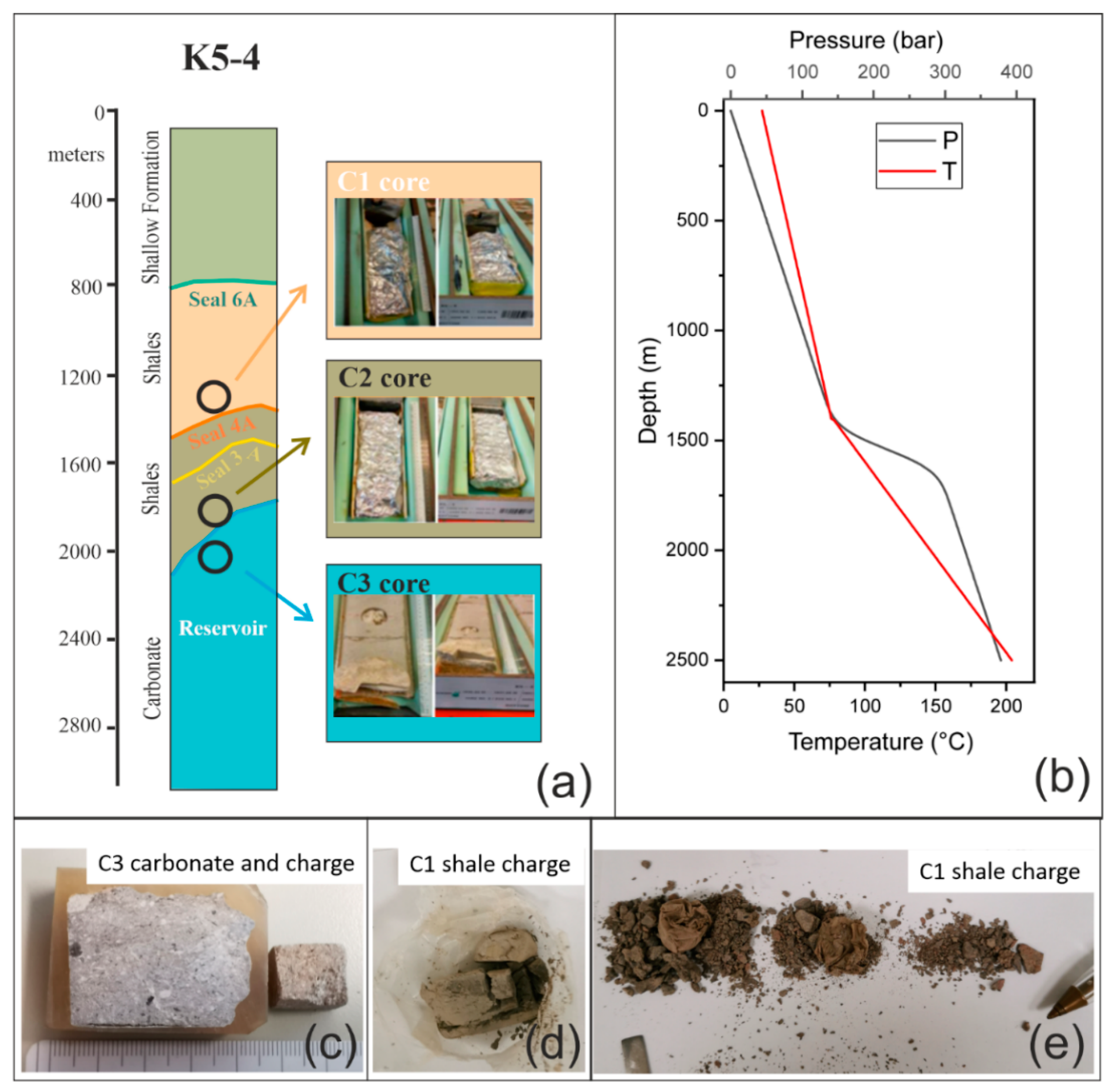
3.1. Cores Characterization

Original petrographic features of core samples were defined at various scales by XRPD, XRF, FT-IR, and SEM-EDS analyses.

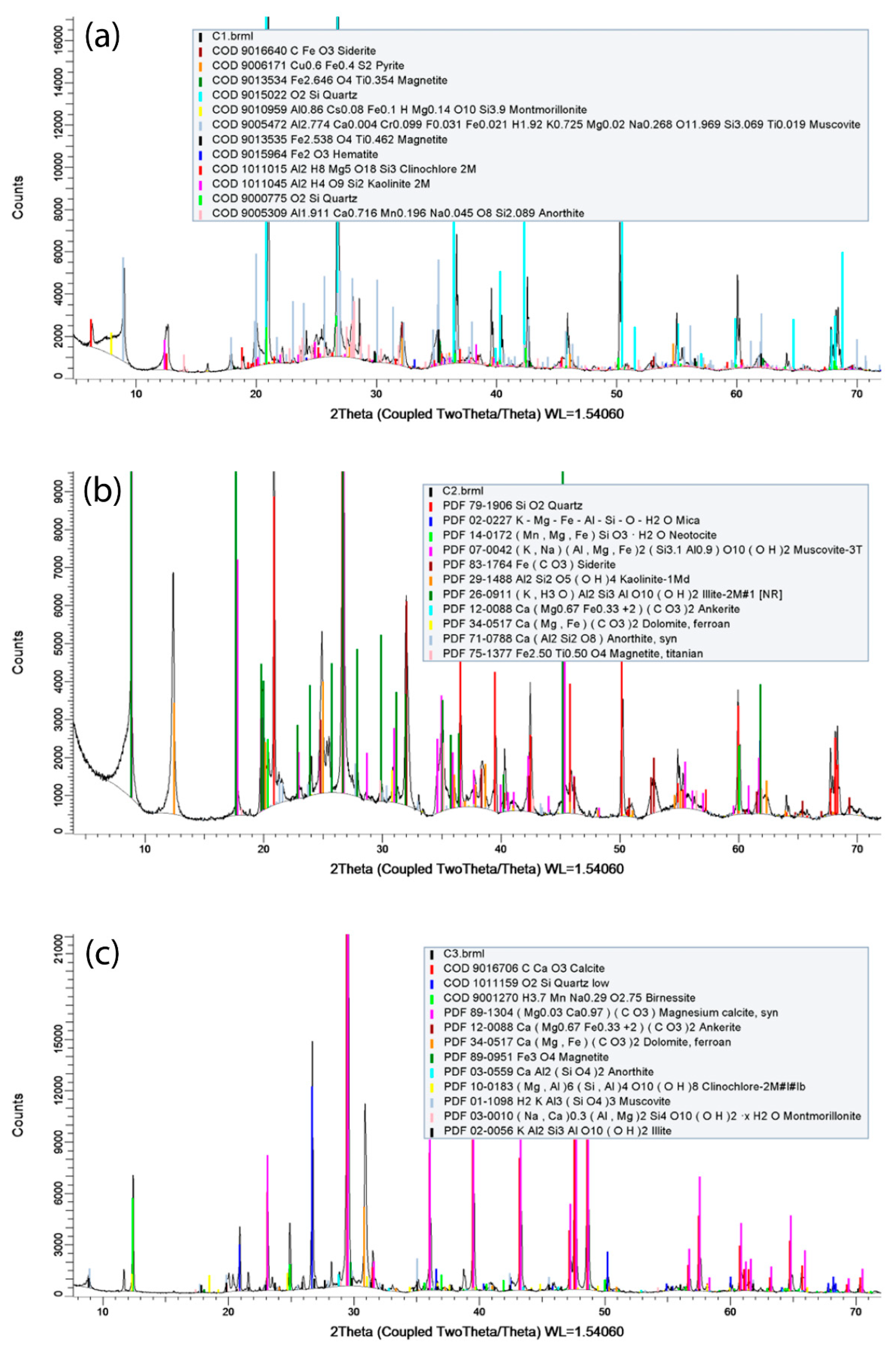
XRPD combined with Rietveld refinement (Figure 3) allowed a semi-quantitative mineralogical composition normalized to 100 (

Table 1. Semi-quantitative mineralogical composition of selected cores (weight %) after Rietveld refinement, normalized to 100.

Minerals	Seal 6	Seal 4	Reservoir
	C1	C2	C3
Quartz	35.96	31.27	10.04
Siderite	4.29	9.64	0.64
Dolomite	2.05	3.16	11.63
Calcite	1.07	1.07	63.94
Ankerite	-	-	<1
Plagioclase	14.98	4.32	2.05
Muscovite	10.83	10.78	1.57
Anatase	<1	-	-
Pyrite	<1	<1	<1
Chlorite	3.04	1.16	1.59
Kaolinite	5.43	14.14	4.70
Illite	22.35	24.46	3.85

-: not present.

). Analytical results show that the shale and shaly silt overburden (C1 and C2 samples) is constituted by ca. 36 and 51% by weight of quartz and plagioclase (anorthite by Rietveld analysis), respectively. Clay minerals (illite, kaolinite and chlorite) contribute from 31 to 40% w/w with minor mica (muscovite) content of 11% w/w. Finally, low amounts of carbonates (calcite, dolomite, and siderite) are present (C1 sample = 7% w/w, C2 sample = 14% w/w). If we compare Seal 6 and Seal 4 samples, this latter shows the major contents of carbonate (14%) and clay minerals (40% w/w) and the minor contents of quartz and anorthite (sand = 36% w/w). The reservoir (C3 sample) is constituted by limestone (76% w/w), mainly calcite and dolomite, subordinate quartz (13% w/w), anorthite and mica, and a very low abundance of clay minerals (10% w/w; illite, chlorite and kaolinite).

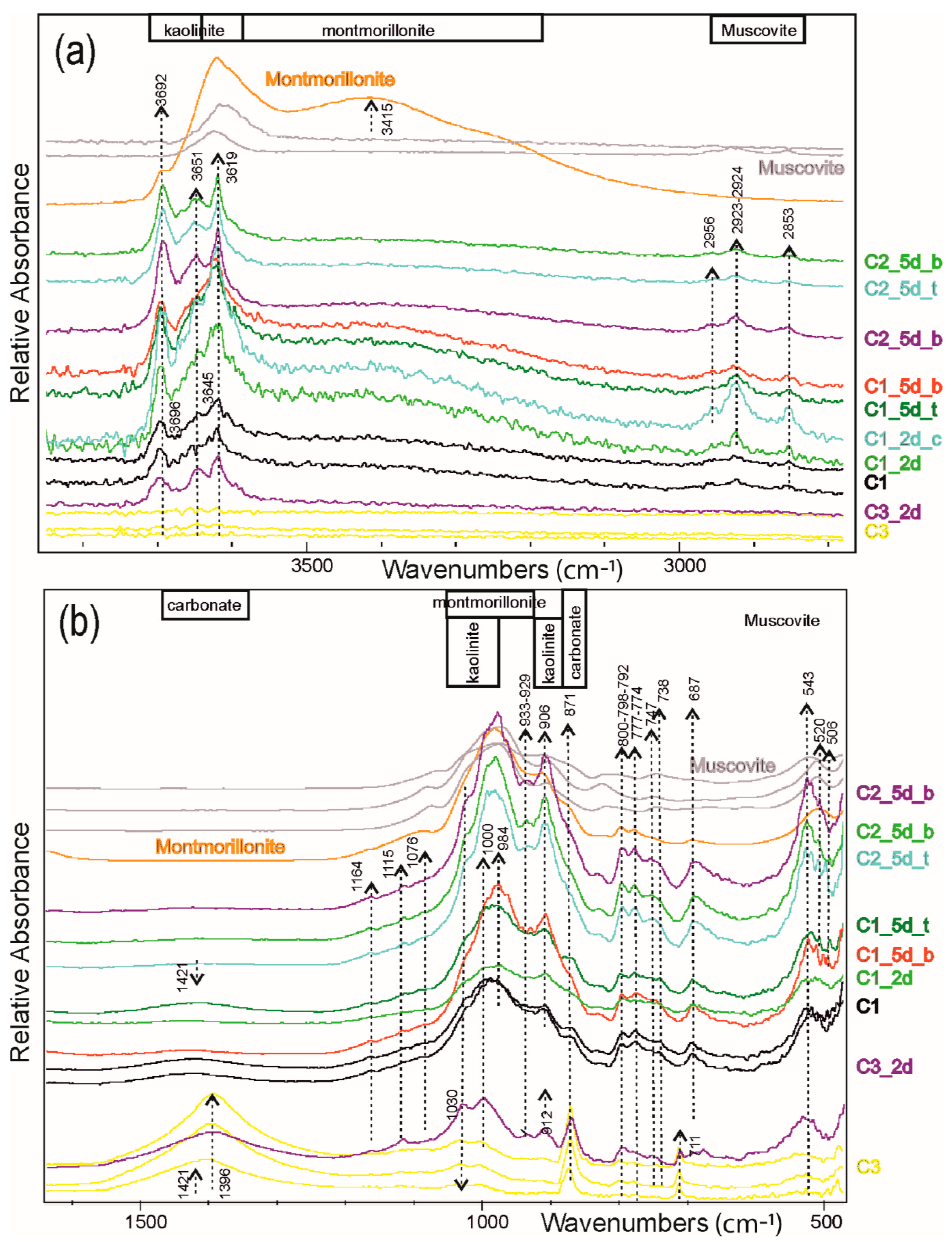
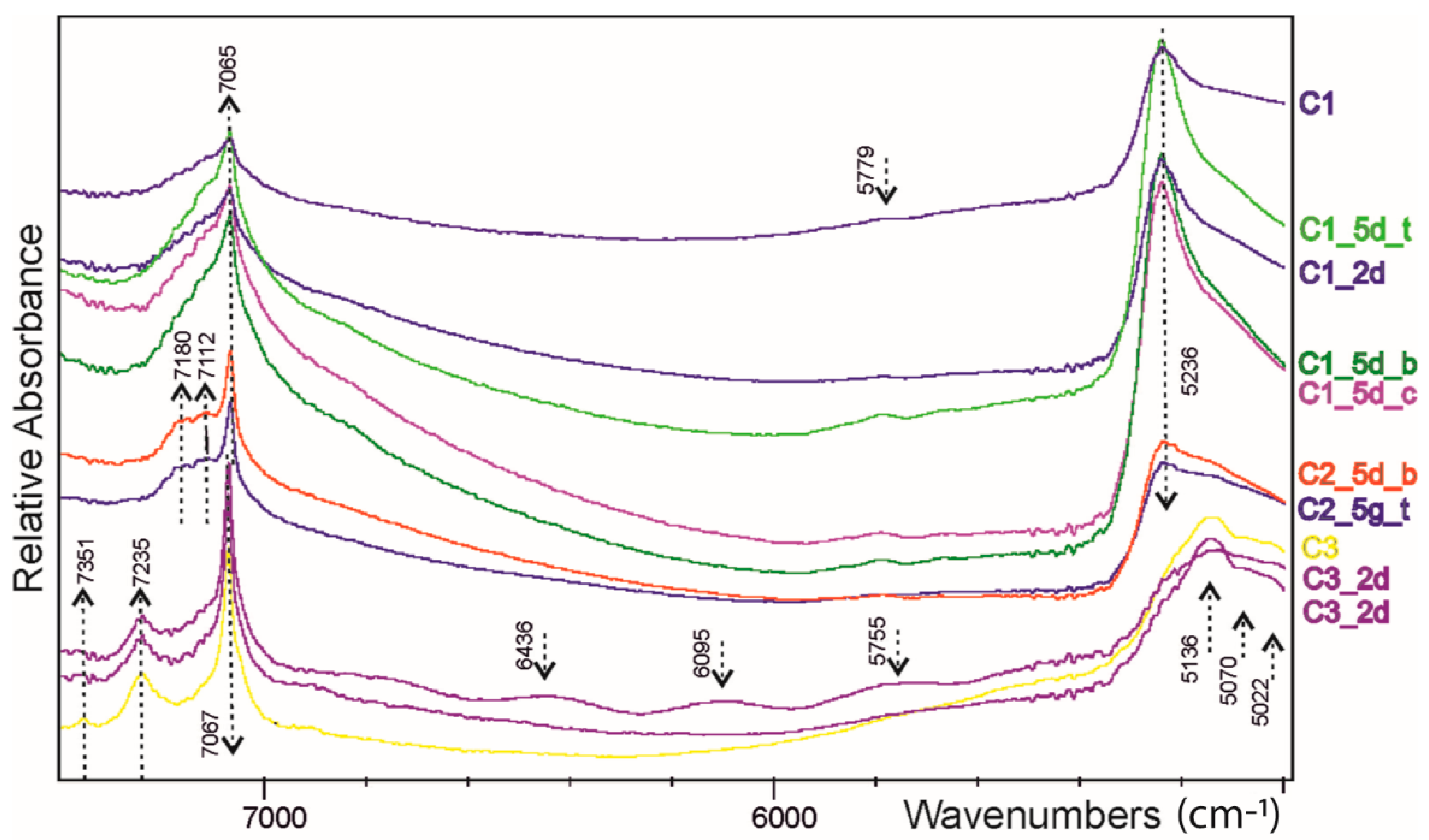
FT-IR spectra (Figure 4 and Figure 5) corroborate the XRPD results indicating carbonate and clay prevalence in the C3 and in the C1 samples, respectively. Actually, the C3 spectrum is dominated by the signals of calcite with typical spikes of absorption bands at 1396 (𝜈₃ CO₃⁻²asymmetrical stretch), 871 (𝜈₂ CO₃⁻²asymmetrical bend) and 711 (𝜈₄ CO₃⁻²aymmetrical bend) cm⁻¹ [23]. A small contribution from the substitution of other (Mg, Fe, Mn) cations can be suspected by comparing the smoothed peak at 5154 cm⁻¹ of our sample with those of siderite (HS271.3B) in the USGS database (https://www.usgs.gov/labs/spectroscopy-lab (accessed on 1 November 2022)). Considering the USGS database, the signals at 7092 and 7246 cm⁻¹ in the carbonate sample highlight the scarce presence of mica and clays, although the doublet at 7246 and 7.092 cm⁻¹ can be tentatively attributed to the kaolinite occurrence. Conversely, for the investigated C1 shale, the illite determines the peaks sequence in the NIR frequency (7092, 5236, 4504, 4255 cm⁻¹) and the shape in the OH-stretching region. In this later range, the mica contribution can be also revealed at ca. 3645 cm⁻¹, as well as the triplet at ca. 2656, 2923, and 2853 cm⁻¹. According to [24,25], several peaks at ca. 1030, 1000, and 984 cm⁻¹ (Si-O stretching), at ca. 933, 906, and 870 cm⁻¹ (vibration of AlAlOH and AlFeOH groups) and at ca. 543, 520, and 506 cm⁻¹ (Al-O and Si-O deformation) can be attributed to clays (mostly illite/montmorillonite and kaolinite). Notably, for C1, the triplet at 2957 + 2922 + 2850 cm⁻¹ and the smoothed signals at 1421 cm⁻¹ point to muscovite being richest and a significant occurrence of (ankerite, dolomite, siderite) carbonates, respectively. Based on the peak at 3619 and the hamp at 3415 cm⁻¹, it is demonstrated that montmorillonite/illite is the major clay in shales.

XRF results are reported in

Table 2. XRF analysis (oxides weight %) of C1, C2 and C3 rock samples.

Oxides	C1	C2	C3	C1-Corrected	C2-Corrected	C3-Corrected
B2O3	2.41	-	2.11	1.61	-	1.41
Na2O	0.81	0.23	0.25	0.54	0.15	0.16
MgO	1.40	1.10	0.81	0.93	0.74	0.54
Al2O3	19.09	22.89	8.90	12.77	15.31	5.95
SiO2	61.49	57.31	19.57	41.12	38.32	13.09
P2O5	0.15	0.15	0.11	0.10	0.10	0.07
SO3	0.50	0.90	1.99	0.34	0.60	1.33
Cl	0.04	0.02	0.24	0.03	0.01	0.16
K2O	3.85	4.25	1.03	2.57	2.84	0.69
CaO	0.82	1.41	60.05	0.55	0.94	40.15
TiO2	1.28	1.13	0.42	0.85	0.76	0.28
V2O5	-	-	0.03	-	-	0.02
Cr2O3	0.05	0.03	0.02	0.03	0.02	0.01
MnO	0.12	0.09	0.03	0.08	0.06	0.02
Fe2O3	7.76	10.25	2.39	5.19	6.85	1.60
NiO	0.013	0.02	0.01	0.01	0.01	0.01
CuO	0.01	0.01	0.01	0.01	0.06	0.01
ZnO	0.02	0.02	0.01	0.01	0.02	<0.01
Rb2O	0.03	0.03	0.01	-	-	<0.001
Ga2O3	-	0.01	-	-	-	-
As2O3	0.01	0.01	-	-	-	-
SrO	0.03	0.04	0.60	0.017	0.03	0.40
ZrO2	0.05	0.03	-	-	-	-
Nb2O5	-	<0.01	-	-	-	-
BaO	0.09	0.07	1.40	0.06	0.05	0.93
PbO	-	-	0.014	-	-	0.01
CO2	-	-	-	3.55	6.55	34.716

Corrected: the compositions were corrected for the contribution of CO₂ loss from carbonates determined by calcimetric analysis.

, also considering CO₂ loss correction. The overburden shales mostly contain SiO₂ (38–41% w/w) and Al₂O₃ (12–16% w/w), with minor amounts of K₂O (2.6% w/w) and Fe₂O₃ (5.2% w/w). Boron and magnesium oxides are also present. Moreover, for XRPD, these oxides suggest the presence of quartz and clay minerals rich in potassium and iron, such as illite, chlorite, and muscovite. In the C3 sample, the most abundant oxide is CaO (40.2% w/w) with minor amounts of SiO₂ (13% w/w), Al₂O₃ (6% w/w), Fe₂O₃ (1.6% w/w), and SO₃ (1.33% w/w). The presence of SO₃ is likely due to pyrite contribution, which was recognized in XRPD but not quantified due to the very low amount.

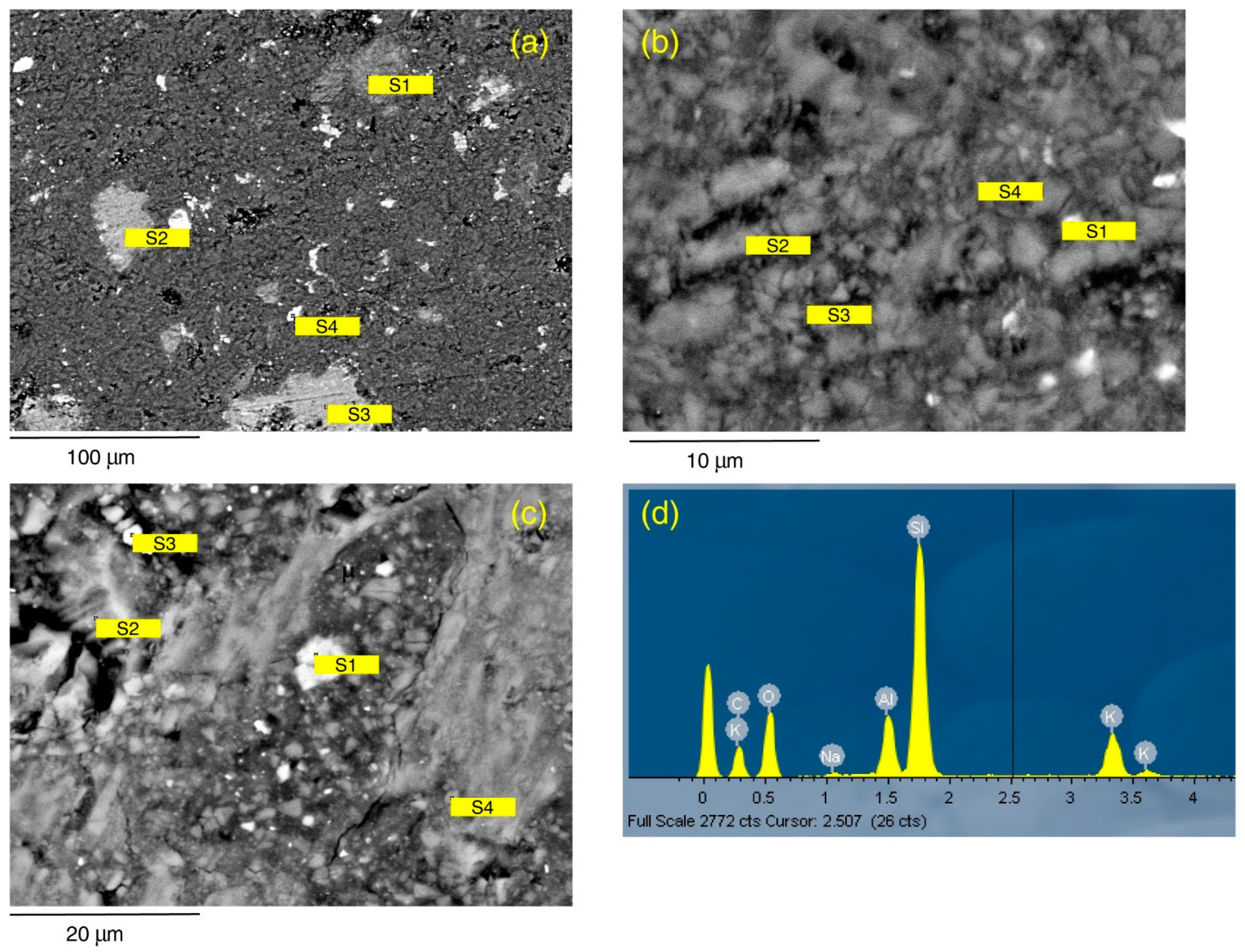
SEM-EDS investigation of Seal 6 shale (C1 sample) at a low magnification scale (Figure 6a) shows the presence of some phenocrysts of muscovite (mean 24 × 33 µm), Fe-rich dolomite-ankerite (mean 24 × 37 µm), and anatase (mean 6 × 12 µm), which are dispersed in a dominant finer matrix. The matrix is cohesive and generally low porous. The total porosity, measured by MICP, is 8.7%, with an asymmetrical distribution of pores and mean frequency of 0.019 μm. Tortuosity is 2.174. The zoom on the matrix (Figure 6b,c) reveals that it is constituted by microcrysts of quartz (mean 1.53 × 2.6 µm), secondary illite (mean 0.7 µm), chlorite (mean 0.93 × 1.33 µm), and kaolinite (mean 0.62 × 3.19 µm). The clay minerals exhibit both spherical and plate like shape. Illite and chlorite are generally rich in iron ion, in variable content ranging from 0.51% to 7.03%, in agreement with marine or hypersaline environments where the sedimentation rate is low. Indeed, the sources of K (for illite) and Fe ions are seawater and detrital minerals, respectively [26]. Cubic siderite-dolomite microcrystals (mean 1.11 × 1.99 µm) are also present. Primary plagioclase (5.5 µm, spectrum 2) and quartz are visible in Figure 6c.

Figure 6. SEM-EDS data of C1 sample in thin section. (a) General aspect at low magnification scale at the analytical Site 1. S1: muscovite with quartz; S2 and S3: solid solution of Fe-rich dolomite and ankerite; S4: anatase. (b) Texture and mineralogy of the analytical Site S2. S1: Fe-rich illite; S2 and S3: quartz; S4: illite. (c) Texture and mineralogy of the analytical Site 3. S1: solid solution of siderite-ankerite; S2: kaolinite with adsorbed Na from underlying primary plagioclase; S3: solid solution of Fe-rich chlorite and illite; S4: kaolinite. (d) EDS spectrum of S1 in panel (a) compatible with mixture of muscovite and quartz. Mineral compositions are related to spectrum for site in Table 3.

Figure 6. SEM-EDS data of C1 sample in thin section. (a) General aspect at low magnification scale at the analytical Site 1. S1: muscovite with quartz; S2 and S3: solid solution of Fe-rich dolomite and ankerite; S4: anatase. (b) Texture and mineralogy of the analytical Site S2. S1: Fe-rich illite; S2 and S3: quartz; S4: illite. (c) Texture and mineralogy of the analytical Site 3. S1: solid solution of siderite-ankerite; S2: kaolinite with adsorbed Na from underlying primary plagioclase; S3: solid solution of Fe-rich chlorite and illite; S4: kaolinite. (d) EDS spectrum of S1 in panel (a) compatible with mixture of muscovite and quartz. Mineral compositions are related to spectrum for site in Table 3.

Table 3. Semi-quantitative analysis of C1 sample in atoms percentage.

Spectrum	Mineral	O	Na	Mg	Al	Si	K	Ca	Ti	Mn	Fe
1-Site1	muscovite + quartz	64.70	0.64	-	5.59	24.15	4.92	-	-	-	-
2-Site1	Fe-dolomite + ankerite	74.57	-	6.64	-	0.52	-	13.38	-	1.21	3.69
3-Site1	Fe-dolomite + ankerite	73.96	-	6.16	-	0.60	-	15.03	-	-	4.25
4-Site1	anatase	68.70	0.67 *	-	0.25 *	0.55 *	-	-	29.83	-	-
1-Site2	Fe-rich illite	65.39	1.12	2.07	6.38	19.25	0.87	0.49	-	-	4.42
2-Site2	quartz	65.45	-	-	0.31 *	34.24	-	-	-	-	-
3-Site2	quartz	66.55	-	-	0.38 *	33.07	-	-	-	-	-
4-Site2	Illite	64.91	1.23	0.56	6.03	25.93	0.83	-	-	-	0.51
1-Site3	siderite-dolomite	68.06	-	7.62	1.82 *	2.92 *	-	1.79	-	-	17.78
2-Site3	kaolinite on primary plagioclase	68.35	4.65	-	7.79	17.56	0.17	1.49	-	-	-
3-Site3	Fe-chlorite+illite	68.84	2.85	3.44	4.81	11.50	-	1.55	-	-	7.03
4-Site3	kaolinite	66.30	2.17	-	5.60	24.52	-	1.23	-	-	0.19

*: Contamination from close by minerals. Refer to Figure 6 for details on spectrum and site number.

Table 3. Semi-quantitative analysis of C1 sample in atoms percentage.

Spectrum	Mineral	O	Na	Mg	Al	Si	K	Ca	Ti	Mn	Fe
1-Site1	muscovite + quartz	64.70	0.64	-	5.59	24.15	4.92	-	-	-	-
2-Site1	Fe-dolomite + ankerite	74.57	-	6.64	-	0.52	-	13.38	-	1.21	3.69
3-Site1	Fe-dolomite + ankerite	73.96	-	6.16	-	0.60	-	15.03	-	-	4.25
4-Site1	anatase	68.70	0.67 *	-	0.25 *	0.55 *	-	-	29.83	-	-
1-Site2	Fe-rich illite	65.39	1.12	2.07	6.38	19.25	0.87	0.49	-	-	4.42
2-Site2	quartz	65.45	-	-	0.31 *	34.24	-	-	-	-	-
3-Site2	quartz	66.55	-	-	0.38 *	33.07	-	-	-	-	-
4-Site2	Illite	64.91	1.23	0.56	6.03	25.93	0.83	-	-	-	0.51
1-Site3	siderite-dolomite	68.06	-	7.62	1.82 *	2.92 *	-	1.79	-	-	17.78
2-Site3	kaolinite on primary plagioclase	68.35	4.65	-	7.79	17.56	0.17	1.49	-	-	-
3-Site3	Fe-chlorite+illite	68.84	2.85	3.44	4.81	11.50	-	1.55	-	-	7.03
4-Site3	kaolinite	66.30	2.17	-	5.60	24.52	-	1.23	-	-	0.19

*: Contamination from close by minerals. Refer to Figure 6 for details on spectrum and site number.

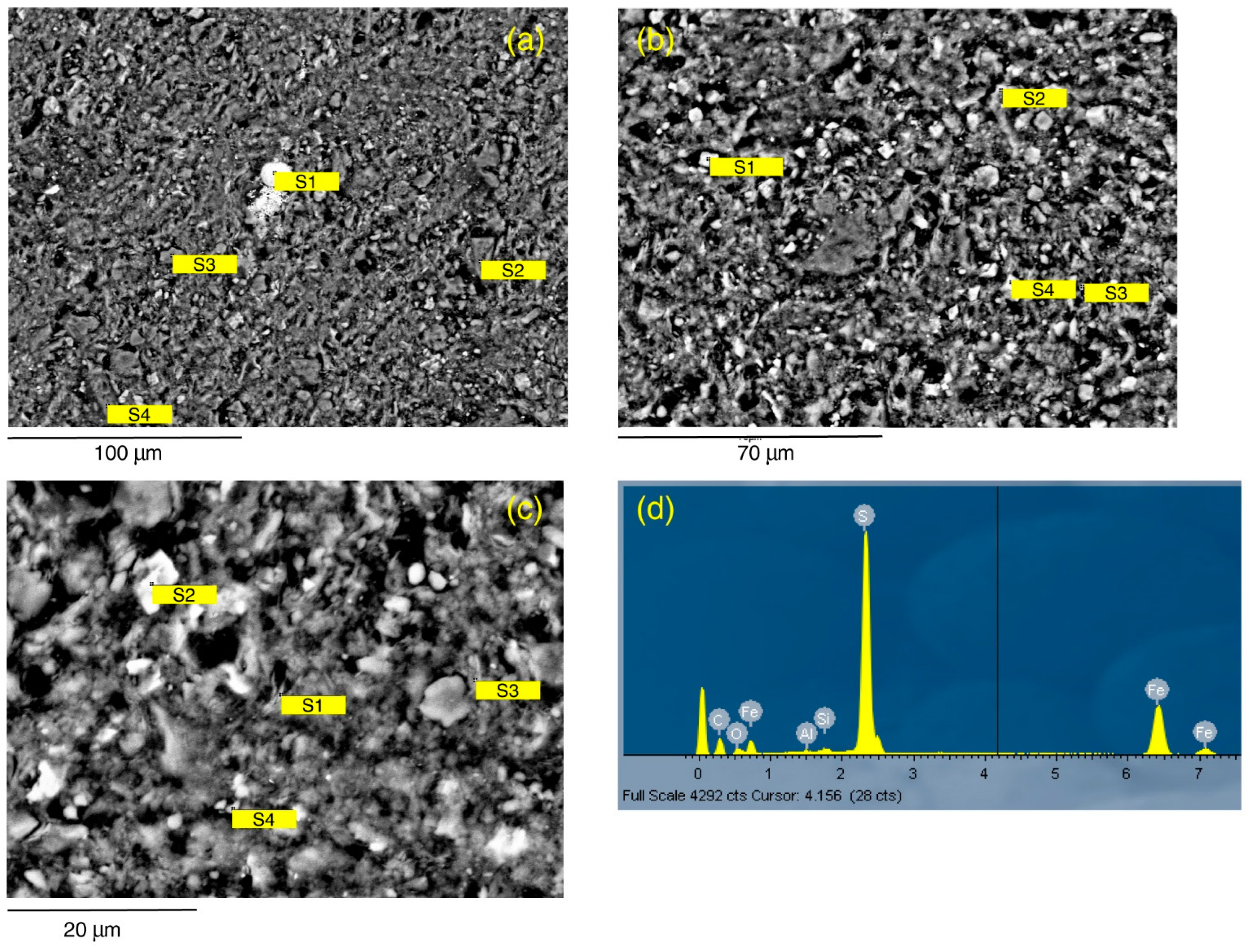
SEM analysis of Seal 4 (C2 sample) at low magnification (Figure 7a) shows a slightly coarser and more porous structure than C1 sample. Based on MICP, this sample has a total porosity of 9.2%, with an average pore distribution of 0.15 μm. Tortuosity is 2.164. At the above spatial scale, only pyrite (mean 10 µm) and quartz macro crystals (mean 4.8 × 12.7 µm) are clearly distinguishable. An enlarged magnification (Figure 7b) allows further distinguishing cubic crystals of dolomite-siderite (mean 2.8 µm), small crystals of anatase (mean 1.6 µm) (

Table 4. Semi-quantitative analysis of C2 sample in atoms percentage.

Spectrum	Mineral	O	Na	Mg	Al	Si	K	S	Ca	Ti	Fe
2-Site1	quartz	68.48	-	-	-	31.52	-	-	-	-	-
3-Site1	quartz	68.45	-	-	0.39 *	31.16	-	-	-	-	-
4-Site1	quartz	66.96	-	-	-	33.04	-	-	-	-	-
1-Site2	dolomite-siderite	74.03	-	9.90	1.16 *	1.76 *	0.20 *	-	2.06	-	10.90
2-Site2	illite	68.57	0.71	0.30	11.84	15.83	2.39	-	-	-	0.36
3-Site2	anatase	73.52	-	-	4.78 *	9.44 *	0.65 *	-	-	11.34	0.26 *
4-Site2	dolomite-siderite	73.38	-	9.69	1.19 *	1.29 *	-	-	2.11	-	12.34
1-Site3	kaolinite	68.56	0.42 *	0.54 *	11.11	17.00	1.86 *	-	-	-	0.51 *
2-Site3	dolomite-siderite	74.49	-	8.40	2.42 *	3.43 *	-	-	1.86	-	9.41
3-Site3	muscovite	68.34	0.44 *	0.31 *	8.80	19.87	1.56	-	-	0.21	0.46
4-Site3	illite-chlorite	70.14	-	2.47	7.95	14.48	1.37	-	0.51	0.25	2.83

*: Contamination from close minerals. Refer to Figure 6 for details on spectrum and site number.

) and, in the matrix, illite, both spherical (mean 2.15 µm) and plate shape (mean 1.18 × 5.05 µm), kaolinite (mean 0.71 × 4.83 µm), and quartz (mean 12 × 19 µm). The zoom on the matrix (Figure 7c, Table 4) shows that it is mostly constituted by secondary illite-chlorite rich in Fe, both spherical (mean 1.62 µm) and plate shape (mean 1.03 × 2.38 µm), kaolinite (mean 0.28 × 1.35 µm), muscovite (mean 0.84 × 2.3 µm), and micro crystals of dolomite-siderite (mean 2.5 µm).

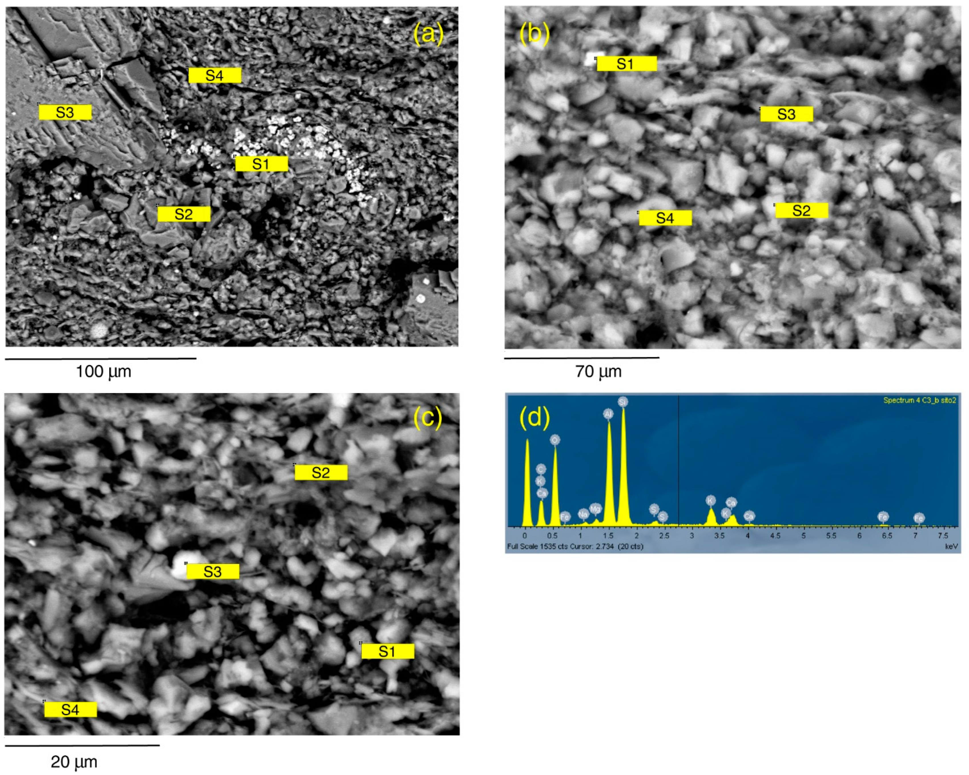
SEM analysis of carbonate reservoir sample (C3) at a low magnification scale (Figure 8a) shows the presence of primary calcite (

Table 5. Semi-quantitative analysis of C3 sample in atoms percentage.

Spectrum	Mineral	O	Na	Mg	Al	Si	K	P	S	Ca	Cl	Ti	Fe
2-Site1	calcite	79.92	-	-	1.85 *	2.85 *	0.32 *	-	0.28*	14.79	-	-	-
3-Site1	kaolinite - illite	74.55	0.49 *	0.39 *	7.06	14.59	1.10 *	-	-	1.45 *	0.18 *	-	0.19 *
4-Site1	quartz	73.69	-	0.27 *	1.43	23.49	0.20 *	-	-	0.92 *	-	-	-
2-Site2	calcite	77.71	-	-	-	0.34 *	-	-	-	21.94	-	-	-
3-Site2	calcite	74.84	-	-	-	-	-	-	-	24.86	0.30 *	-	-
4-Site2	kaolinite-illite	69.35	0.45 *	0.59 *	11.01	14.47	2.06	-	0.46 *	1.31	-	-	0.31
1-Site3	kaolinite	75.92	-	-	9.53	13.07	0.20 *	-	-	1.17 *	-	-	0.11
2-Site3	illite	71.24	0.27	0.51	9.75	14.88	1.35	0.28	-	1.48	-	-	0.23
4-Site3	muscovite	72.98	-	0.87	7.88	13.07	2.10	-	-	2.38 *	-	0.26	0.46

*: Contamination from close minerals. Refer to Figure 6 for details on spectrum and site number.

) and clay with a plate-like structure (mean 0.5 × 2.23 µm). The porosity, as measured by MICP, is 9.4%, close to the C2 sample but C3 has a more symmetrical distribution, with average porous dimension ranging from 0.0723 to 0.0792 μm. Tortuosity is 2.125. A fossil re-crystallized by small crystals of pyrite (mean 1 µm) is present in the center of the picture. The zoom on the matrix (Figure 8b,c) reveals that it is constituted by secondary calcite (mean 2.19 µm), kaolinite (mean 0.8 × 6.4 µm), illite (mean 1.2 × 4.75 µm), muscovite (mean 0.52 × 5.7 µm), and quartz (mean 0.92 × 4.2 µm). Rare crystals of pyrite (3–5 µm) and sylvite are also present.

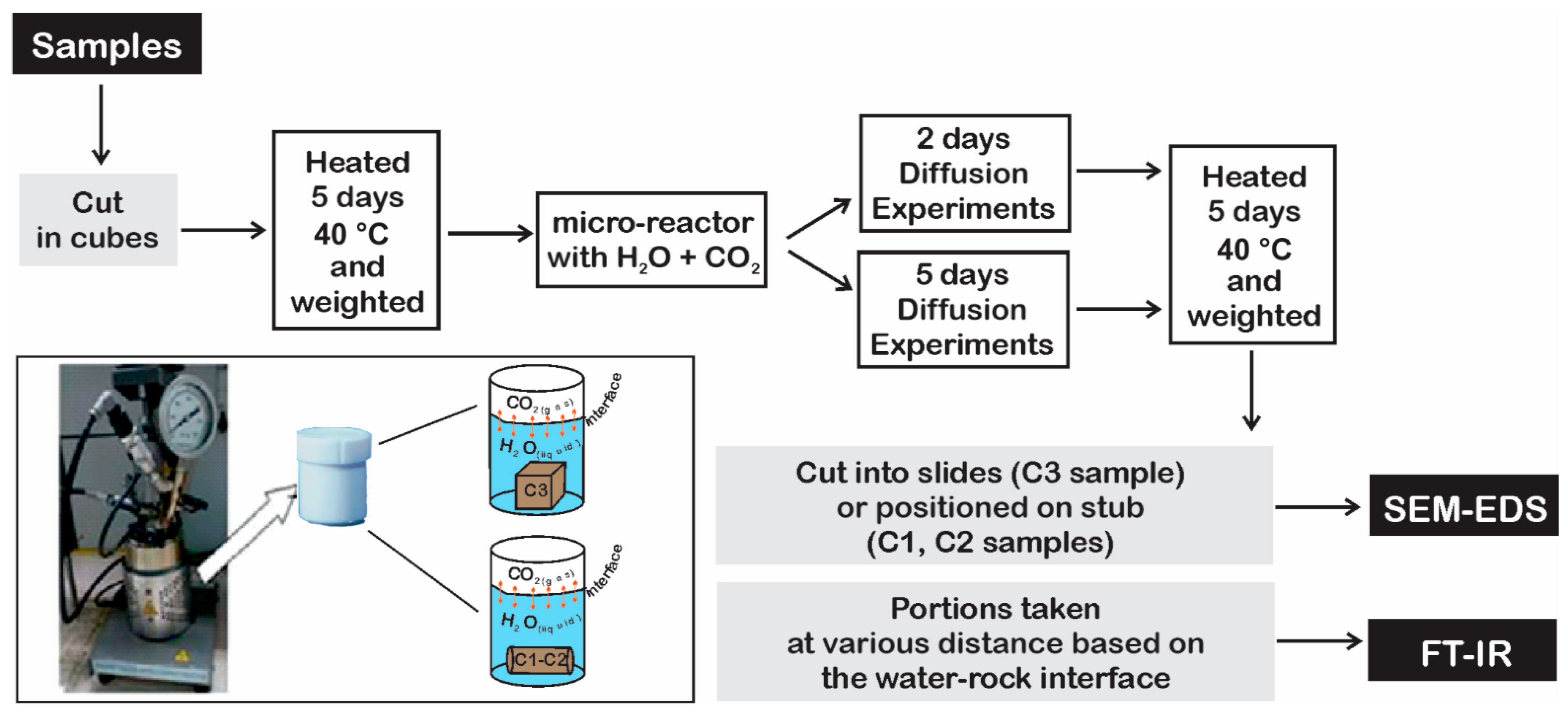
3.2. Diffusion Experiments

The reaction front due to fluid–rock interaction was evaluated by SEM-EDS analysis after two and five days of interaction inside the micro-reactor. As expected, due to the short interaction time, the results indicate limited sample changes that mostly concerned with carbonates and pyrite.

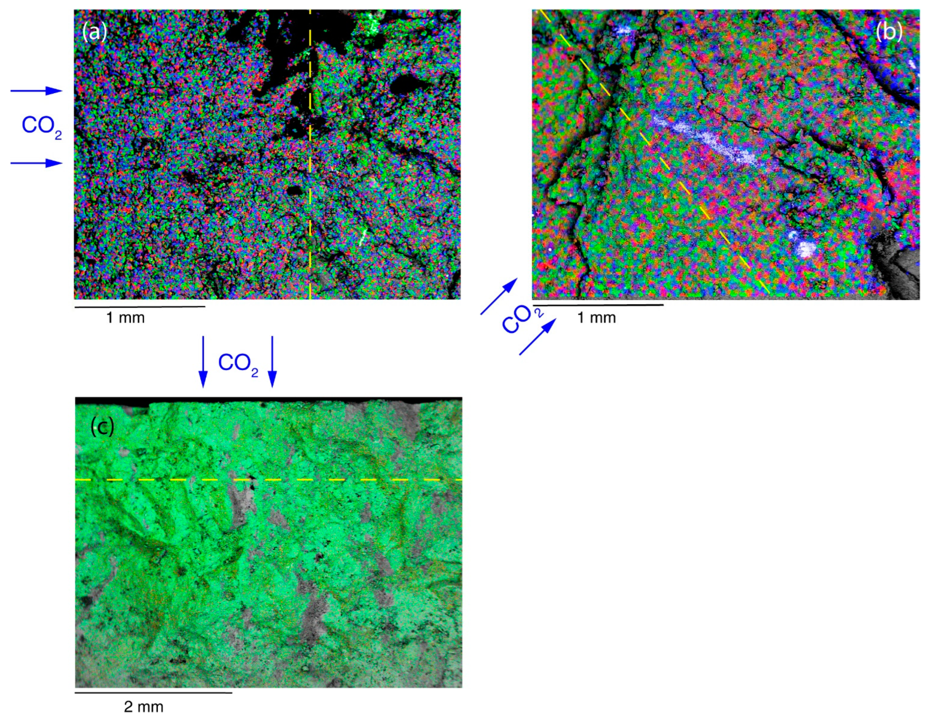
SEM-EDS investigations were conducted in two modes: (i) classical electron microscope image (e.g., Figure 9), and (ii) chemical map (cameo image) by chemical fake-coloring (Figure 10). The color scale was arbitrarily changed to highlight the reaction front, thus not reflecting the real abundance of the elements. The first analysis aimed to recover chemical changes and to spot secondary minerals, whereas the cameo images were used to define the boundary between unaltered sample and the weathering due to CO₂ reaction.

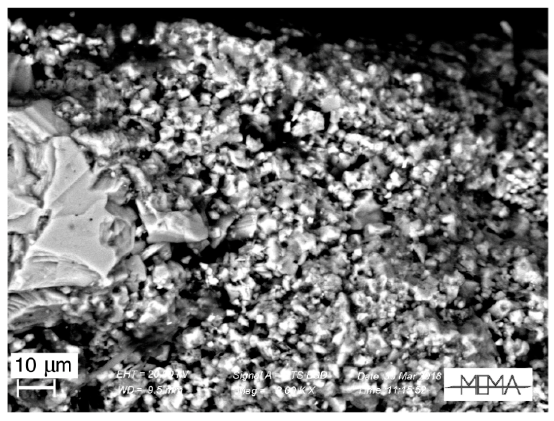
A general feature observed on the SEM images after the experiments is the depletion in the pyrite microcrystals and a relative increased abundance of carbonates mostly in the form of micron sized cubes (Figure 9). These carbonates, still pertaining to the dolomite-siderite-ankerite series, generally resulted depleted in Ca in favor of Mg and Fe at the EDS, exhibiting an evident rhombohedral habit (C3 sample, Figure 11) and believed to represent secondary phases. Figure 10a (C1 sample) shows this phenomenon, with a relative enrichment of Fe and Mg (red and blue colors, respectively) with respect to Ca (green color) in the portion of the specimen which reacted with CO₂. In Figure 10b (C2 sample) a relative enrichment of Mg (green) is visible within the reaction area. The Mg relative enrichment and false scale color jeopardize the original major abondance of Fe and K (visible on the other side of reaction front) of C2 with respect to C1 samples. The reaction front of C3 sample (Figure 10c) is slightly evident since Ca and Mg are the major elements constituting carbonates. The green color represents the iron content, which is more evident in the unaltered sample portion, thus allowing the front identification by the color intensity. The different coloring across the reaction front is due to the weathering process, which occurs as CO_2(aq) reached the minerals, and its effect on the coloring is not easily predictable, since it could be due to both matrix depletion after weathering and/or subsequent deposition of leached elements.

The distribution of minerals and elements at mm-scale allows to define two reaction fronts, the first corresponding to the area of pyrite depletion and the second coinciding with the precipitation of secondary carbonates.

The distance of these fronts from the outer part of the specimen allows defining the CO₂ penetration depth (e.g., Figure 9) after two and five days. These distances were measured by SEM ruler, whose instrumental accuracy is within 1 µm, but considering the difficulties in localizing the alteration front and its unevenness, we can reasonably estimate the experimental error to be approximately 10 µm. The measured penetration front and the depletion front length are reported in

Table 6. Diffusion coefficients obtained from experiments.

	Temperature, °C	Penetration Length, mm	Depletion Length, mm	Draw, m2s−1	De, m2s−1
C1
2 days	75	2.99 ± 0.01	0.67 ± 0.01	5.17 ± 0.035 × 10−11	9.77 × 10−11
5 days	75	3.48 ± 0.01	1.48 ± 0.01	2.80 ± 0.016 × 10−11
C2
2 days	105	2.60 ± 0.01	0.66 ± 0.01	3.91 ± 0.03 × 10−11	1.53 × 10−10
5 days	105	3.50 ± 0.01	1.24 ± 0.01	2.84 ± 0.016 × 10−11
C3
2 days	145	2.41 ± 0.01	1.44 ± 0.01	3.36 ± 0.028 × 10−11	2.51 × 10−10
5 days	145	3.67 ± 0.01	0.94 ± 0.01	3.12 ± 0.017 × 10−11

.

FT-IR spectra in Figure 4 and Figure 5 indicate no significant variation in shales subjected to diffusion experiments, whereas after two days of hydrothermal action, the C3 carbonate significantly modified its infrared response. In particular, several peaks appeared in the OH- stretching region and between 1500 and 500 cm⁻¹ of the experimental C3 sample, i.e., at ca. 3695, 3648, 3633, 3618, 932–910, 540–470 cm⁻¹(Figure 4), pointing to kaolinite plus illite/muscovite [24,25,27]. The doublet at 3695 and 3618 cm⁻¹ is diagnostic for the kaolin phase and is corroborated by absorption at 933–929 and 906 cm⁻¹ (OH-bending/vibrations). The illite/muscovite is indicated by signals at ca. 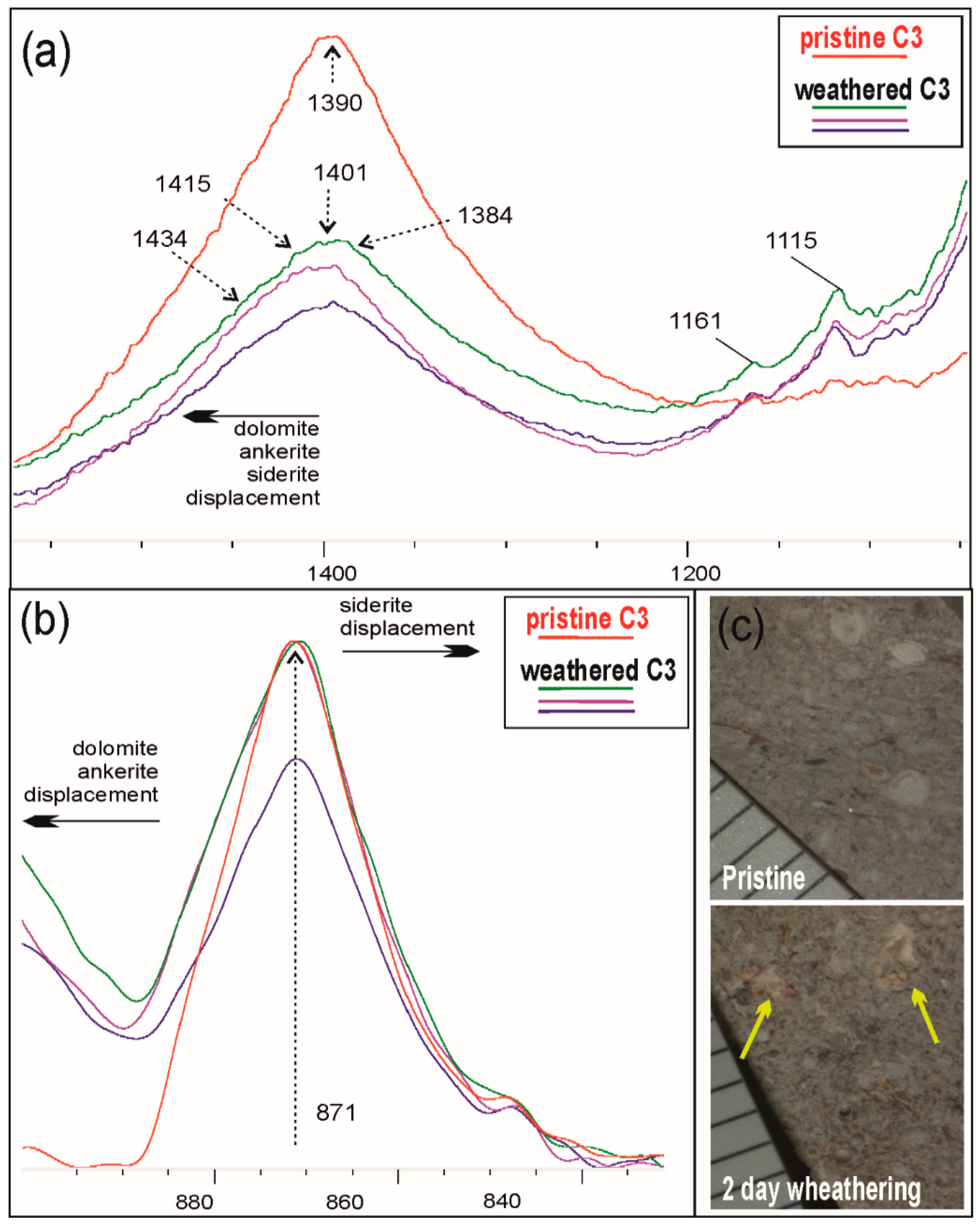1030, 912, and 520 cm⁻¹. The spectra also show a span of both 𝜈₃ CO₃²⁻ asymmetrical stretch and bend bands, the first band assuming a bell-shaped between 1384 and 1434 cm⁻¹ and the second slightly distorting towards higher and lower wavenumbers (Figure 12a,b). Following [23], this indicates Mg, Fe carbonate and, in our case, may suggest calcite dissolution in agreement with the experimental sample aspect under the optical microscope (Figure 12c). Notably, shales are slightly different, maintaining the more accentuated peaks at 3651, 3619, and 932 cm⁻¹ for the kaolinite abundance in sample C2, and for C1, the triplet at 2957 + 2922 + 2850 cm⁻¹ for muscovite being richest, and the smoothed signals at 1421 cm⁻¹ for the occurrence of ankerite, dolomite, and siderite carbonates, in addition to the illite (3622 and 3415 cm⁻¹). However, in these experimental samples, the infrared signals at 800, 777, and 747 cm⁻¹ (Figure 4) show faint but sensible variations that would be interest to OH bending vibrations/interactions with cations, thus pointing to possible leeching processes. The 1000 and 900 cm⁻¹ bands, related to Si-O-Si stretching and Al-Al-OH bending [28], can be tentatively attributed to structural modification of the illite clays or muscovite with possibly consequent cation losses.

4. Discussion

The performed study aimed to explore the penetration depth and time of CO₂ during hydrothermal experiments. Despite the limitations presented by the analytical strategy and experimental samples, the obtained results show fast reactive minerals alteration.

A few (two and five) days allows the weathering of only fast reactive minerals, i.e., carbonate, sulfides, and sulfates [29], and a possible leaching from clays. In fact, we observed major alteration in the C3 carbonate sample and minor changes in the C1 and C2 shales, in all cases mainly concerning carbonates and pyrite. Based on the both SEM-EDS and FT-IR results, ankerite is more represented in altered samples as results of dissolution of calcite or of carbonate dissolution and recrystallization. In this latter case, carbonate traps Fe+Mg>Ca with the iron released by disappeared pyrite, although we can guess that some iron is originated from the leaching of Fe-rich minerals. An oxidation process during the experiments, which could be responsible of pyrite depletion, is unlikely since all oxygen was removed by using disareated water and flushing the cell with pure CO₂. Moreover, no sulfate phase was observed. The carbonate dissolution determines a relative sample enrichment in clay (kaolinite over montmorillonite and illite). In the shales, the FT-IR spectra suggest that experiments produced modification of the illite/muscovite structure, likely releasing cations.

The mineralogical changes in the matrix after two and five days are attributed to the action of CO₂ penetrated in the samples. Considering geochemical reactions, the distance of the penetration front and depletion front from the outer edge of the specimens was defined, with an estimated experimental error of approximately 10 µm (Table 6).

The penetration length L (m) over the time t (s) may be used to roughly compute the apparent diffusion coefficient D_raw (m² s⁻¹) according to Equation (1) (Table 6). This rough evaluation should be conducted only for the penetration length, while the second front observed in the diffusion experiment is related to mineral depletion and should be better described by geochemical modeling.

$$D_{raw}=\frac{L^2}{t}$$

(1)

Equation (1) is a simple relationship between the only two parameters, L and t, we can measure by SEM images after the experiments. Equation (1) derives from the analytical solution of diffusion equation in one dimension and has been already used to evaluate the apparent diffusion coefficient in cements after experiments with CO₂ by [30,31,32].

The proposed approach is different from the computation of the effective diffusivity of CO₂ in a porous media, D_e (m² s⁻¹), considering the CO₂ diffusion coefficient in water (D_w, m² s⁻¹), porosity (φ), and tortuosity (τ) (Equation (2)).

Indeed, in our case, the diffusivity values computed by Equation (1) are ruled by CO₂⁻ induced reactions, whereas those computed by Equation (2) (Table 6) can refer only to unreacted sample, and a more complex model accounting for geochemical reactions should be performed to obtain an accurate computation instead of Equation (2). The difference in diffusive transport properties between unaltered and altered rocks can be significant, as shown by [33] for shale caprocks.

$$D_e=\frac{\varphi }{{\tau }^2}{D}_w$$

(2)

where D_raw and D_e computed for C1, C2, and C3 samples are reported in Table 6, where D_w values were taken from [34] at 75 °C, 105 °C, and 145 °C, and φ and τ values were measured by MICP tests on original core samples (see Section 3.1).

Estimated apparent diffusion coefficients for both two- and five-day experiments (with five-day experiments that should prove to be more reliable) range from 2.80 × 10⁻¹¹ m² s⁻¹ to 5.18 × 10⁻¹¹ m² s⁻¹ for shale samples, and from 3.11 × 10⁻¹¹ to 3.36 × 10⁻¹¹ m² s⁻¹ for carbonate. The experimental error ranges from 1.6 × 10⁻¹³ m² s⁻¹ to 3.5 × 10⁻¹³ m² s⁻¹ and its impact on diffusion coefficients may be considered limited.

D_raw values of shales and carbonate are of the same magnitude, with those of shales being slightly higher than carbonate for two-day experiments, whereas after five days, D_raw is higher in C3 than C1 and C2. [35] showed that changes in transport properties in limestones could be affected also by a redistribution of calcite within the sample, as well as weathering of siliciclastic and clay minerals. Computed D_raw values are in agreement with previously published data for shale samples, ranging from 3.08 × 10⁻¹¹ up to 7.80 × 10⁻¹¹ m² s⁻¹ [35,36,37,38,39] (

Table 7. Diffusion coefficients for shales and marlstones reported in literature.

T, °C	De, m2 s−1	Reference
50	3.08 × 10−11	[36]
50	4.81 × 10−11
28	7.80 × 10−11 − 1.2 × 10−10	[35]
	1.20 × 10−11	[38]
20	3 × 10−11	[33]
	4–8 × 10−11	[39]
T, °C	D_CO2(aq), m2 s−1	Reference
25	2.233 × 10−09	[34]
50	3.718 × 10−09
75	5.391 × 10−09
100	7.521 × 10−09
150	12.33 × 10−09

). Differences in the values, within the same order of magnitude, can be due to several factors. First of all, depending on mineral assemblage, dissolution and precipitation may change pore network characteristics. [33] demonstrated a D_e increasing in shales from 5 × 10⁻¹² m² s⁻¹ to 1.9 × 10⁻¹¹ m² s⁻¹ due to redox-sensitive and carbonate reactions. Moreover, CO₂ sorption processes on shales may retard the diffusion front depending on organic materials, clay minerals, and micropore structure [36]. Furthermore, the effective diffusivity depends on experimental temperature and PCO₂, since CO₂ diffusion in water increases with them [34].

Computed effective diffusion coefficients are 9.77 × 10⁻¹¹ m² s⁻¹ for C1, 1.53 × 10⁻¹¹ m² s⁻¹ for C2, and 2.51 × 10⁻¹⁰ m² s⁻¹ for C3 sample. These values are from half to an order of magnitude higher than D_raw diffusivity ones, highlighting the important contribution of chemical reactions in retarding CO₂ diffusivity throughout hosting rock since CO_2(aq) is consumed by chemical reaction and adsorption.

Not many experimental laboratories deal with the complex topic of measuring the effect of geochemical reactions on the CO₂ diffusion coefficient. This is mostly because the results (Table 7) are two orders of magnitude lower than CO_2(aq) molecular diffusion in pure water, mainly due to pore network changes and chemical reactions.

5. Conclusions

Diffusive reaction experiments were carried out on two shales and a carbonate rock sample belonging to an offshore structure in the Malaysian basin with the goals to evaluate the geochemical reactions induced by CO₂ and quantify the CO₂ reaction front velocity in the caprock and reservoir at the respective in-situ temperature conditions. Detailed laboratory analysis, performed before and after diffusion experiments, allowed to characterize the texture, chemistry, and mineral association of rock samples.

Results obtained using SEM-EDS illustrate a general behavior of samples with the alteration of pyrite in favor of carbonate secondary minerals belonging to siderite-ankerite series, along two identified reaction fronts.

FT-IR spectra clearly show the carbonate dissolution/precipitation processes, and point out illite structure changes, likely leading to the loss of cations, in shale samples.

The diffusion coefficients estimated by the penetration length of CO₂ are two orders of magnitude lower than CO_2(aq) molecular diffusion in pure water.

D_raw coefficients have the same magnitude order of the coefficient reported for similar samples in the recent literature, and from half to an order of magnitude lower than D_e computed on an unaltered sample. These differences are mainly imputed to gas–water–rock reactions and adsorption process in shales, which retard the diffusion front.

Results obtained in this study provide an insight concerning the mineralogy of Seal 6, Seal 4, and reservoir formations and represent a discussion point on the obtained diffusion coefficients. Carbon dioxide that migrates from the reservoir into the cap rock reacts with minerals, hence reducing the slow, diffusion-driven migration.

Obtained information here reported may be also useful to set up future numerical simulations of reactive transport flow in geological structures potentially suitable for CO₂ storage.

References

1. Metz, B. Carbon Dioxide Capture and Storage: Special Report of the Intergovernmental Panel on Climate Change; Cambridge University Press: Cambridge, UK, 2005. [Google Scholar]
2. Metz, B.; Davidson, O.R.; Bosh, P.; Dave, R.; Meyer, L.A. Contribution of Working Group III to the Fourth Assessment Report of the Intergovernmental Panel on Climate Change, 2007; Cambridge University Press: Cambridge, UK; New York, NY, USA, 2007. [Google Scholar]
3. IEA Greehouse Gas R&D Programme. Natural and Industrial Analugues for Geological Storage of Carbon Dioxide; IEA Greehouse Gas R&D Programme: Cheltenham, UK, 2009. [Google Scholar]
4. Pachauri, R.K.; Meyer, L.A. IPCC, 2014: Climate Change 2014: Synthesis Report. Contribution of Working Groups I, II and III to the Fifth Assessment Report of the Intergovernmental Panel on Climate Change; IPCC: Geneva, Switzerland, 2014. [Google Scholar]
5. Pruess, K.; García, J. Multiphase Flow Dynamics during CO2 Disposal into Saline Aquifers. Environ. Geol. 2002, 42, 282–295. [Google Scholar] [CrossRef]
6. Rutqvist, J.; Tsang, C.-F. A Study of Caprock Hydromechanical Changes Associated with CO2-Injection into a Brine Formation. Environ. Geol. 2002, 42, 296–305. [Google Scholar] [CrossRef]
7. Damen, K.; Faaij, A.; van Bergen, F.; Gale, J.; Lysen, E. Identification of Early Opportunities for CO2 Sequestration—Worldwide Screening for CO2-EOR and CO2-ECBM Projects. Energy 2005, 30, 1931–1952. [Google Scholar] [CrossRef]
8. Voltattorni, N.; Sciarra, A.; Caramanna, G.; Cinti, D.; Pizzino, L.; Quattrocchi, F. Gas Geochemistry of Natural Analogues for the Studies of Geological CO2 Sequestration. Appl. Geochem. 2009, 24, 1339–1346. [Google Scholar] [CrossRef]
9. Balashov, V.N.; Guthrie, G.D.; Lopano, C.L.; Hakala, J.A.; Brantley, S.L. Reaction and Diffusion at the Reservoir/Shale Interface during CO2 Storage: Impact of Geochemical Kinetics. Appl. Geochem. 2015, 61, 119–131. [Google Scholar] [CrossRef]
10. Gunter, W.D.; Perkins, E.H.; McCann, T.J. Aquifer Disposal of CO2-Rich Gases: Reaction Design for Added Capacity. Energy Convers. Manag. 1993, 34, 941–948. [Google Scholar] [CrossRef]
11. Shafeen, A.; Carter, T. Geological Sequestration of Greenhouse Gases. In Environmentally Conscious Fossil Energy Production; Kutz, M., Elkamel, A., Eds.; John Wiley & Sons, Inc.: Hoboken, NJ, USA, 2009; pp. 207–241. ISBN 978-0-470-43274-7. [Google Scholar]
12. Amann-Hildenbrand, A.; Bertier, P.; Busch, A.; Krooss, B.M. Experimental Investigation of the Sealing Capacity of Generic Clay-Rich Caprocks. Int. J. Greenh. Gas Control. 2013, 19, 620–641. [Google Scholar] [CrossRef]
13. Shogenov, K.; Shogenova, A.; Vizika-Kavvadias, O.; Nauroy, J.-F. Experimental Modeling of CO2-Fluid-Rock Interaction: The Evolution of the Composition and Properties of Host Rocks in the Baltic Region: EXPERIMENTAL MODELING OF CO2 STORAGE. Earth Space Sci. 2015, 2, 262–284. [Google Scholar] [CrossRef]
14. Masoudi, R.; Jalil, M.A.A.; Press, D.; Lee, K.H.; Tan, C.P.; Anis, L.; Darman, N.; Othman, M. An Integrated Reservoir Simulation-Geomechanical Study on Feasibility of CO2 Storage in M4 Carbonate Reservoir, Malaysia. In Proceedings of the Society of Petroleum Engineers—International Petroleum Technology Conference 2012, IPTC 2012, Bangkok, Thailand, 7–9 February 2012; Volume 3, pp. 2583–2600. [Google Scholar] [CrossRef]
15. Piochi, M.; Cantucci, B.; Montegrossi, G.; Currenti, G. Hydrothermal Alteration at the San Vito Area of the Campi Flegrei Geothermal System in Italy: Mineral Review and Geochemical Modeling. Minerals 2021, 11, 810. [Google Scholar] [CrossRef]
16. Cantucci, B.; Montegrossi, G.; Buttinelli, M.; Vaselli, O.; Scrocca, D.; Quattrocchi, F. Geochemical Barriers in CO2 Capture and Storage Feasibility Studies. Transp. Porous Med. 2015, 106, 107–143. [Google Scholar] [CrossRef]
17. Doust, H. Geology and Exploration History of Offshore Central Sarawak. In Energy Resources of the Pacific Region; American Association of Petroleum Geologists: Tulsa, OK, USA, 1981; ISBN 978-1-62981-180-2. [Google Scholar]
18. Vahrenkamp, V.C. Miocene Carbonates of the Luconia Province, Offshore Sarawak: Implications for Regional Geology and Reservoir Properties from Strontium-Isotope Stratigraphy. BGSM 1998, 42, 1–13. [Google Scholar] [CrossRef]
19. Ho, K.F. Stratigraphic Framework for Oil Exploration in Sarawak. Bull. Geol. Soc. Malays. 1978, 10, 1–13. [Google Scholar] [CrossRef]
20. Shapiro, L.; Brannock, W.W. Rapid Analysis of Silicates, Carbonates and Phosphate Rocks; US Government Printing Office: Washington, DC, USA, 1962.
21. Lutterotti, L.; Bortolotti, M.; Ischia, G.; Lonardelli, I.; Wenk, H.R. Rietveld Texture Analysis from Diffraction Images. Z. Fur Krist. Suppl. 2007, 1, 125–130. [Google Scholar] [CrossRef]
22. Wigand, M.; Carey, J.W.; Schütt, H.; Spangenberg, E.; Erzinger, J. Geochemical Effects of CO2 Sequestration in Sandstones under Simulated in Situ Conditions of Deep Saline Aquifers. Appl. Geochem. 2008, 23, 2735–2745. [Google Scholar] [CrossRef]
23. Kim, Y.; Caumon, M.-C.; Barres, O.; Sall, A.; Cauzid, J. Identification and Composition of Carbonate Minerals of the Calcite Structure by Raman and Infrared Spectroscopies Using Portable Devices. Spectrochim. Acta Part A Mol. Biomol. Spectrosc. 2021, 261, 119980. [Google Scholar] [CrossRef]
24. Madejová, J.; Komadel, P. Baseline studies of the clay minerals society source clays: Infrared methods. Clays Clay Miner. 2001, 49, 410–432. [Google Scholar] [CrossRef]
25. Madejová, J. FTIR Techniques in Clay Mineral Studies. Vib. Spectrosc. 2003, 31, 1–10. [Google Scholar] [CrossRef]
26. Meunier, A.; El Albani, A. The Glauconite-Fe-Illite-Fe-Smectite Problem: A Critical Review. Terra Nova 2007, 19, 95–104. [Google Scholar] [CrossRef]
27. Vaculíková, L.; Plevová, E. Identification of Clay Minerals and Micas in Sedimentary Rocks. Acta Geodyn. Geomater. 2005, 2, 167–175. [Google Scholar]
28. Di Pietro, S.A.; Emerson, H.P.; Katsenovich, Y.P.; Johnson, T.J.; Francis, R.M.; Mason, H.E.; Marple, M.A.; Sawvel, A.M.; Szecsody, J.E. Solid Phase Characterization and Transformation of Illite Mineral with Gas-Phase Ammonia Treatment. J. Hazard. Mater. 2022, 424, 127657. [Google Scholar] [CrossRef]
29. Palandri, J.L.; Kharaka, Y.K. A Compilation of Rate Parameters of Water-Mineral Interaction Kinetics for Application to Geochemical Modeling; Geological Survey: Menlo Park, CA, USA, 2004.
30. Kutchko, B.G.; Strazisar, B.R.; Dzombak, D.A.; Lowry, G.V.; Thaulow, N. Degradation of Well Cement by CO2 under Geologic Sequestration Conditions. Environ. Sci. Technol. 2007, 41, 4787–4792. [Google Scholar] [CrossRef] [PubMed]
31. Huet, B.M.; Prevost, J.H.; Scherer, G.W. Quantitative Reactive Transport Modeling of Portland Cement in CO2-Saturated Water. Int. J. Greenh. Gas Control. 2010, 4, 561–574. [Google Scholar] [CrossRef]
32. Hernández-Rodríguez, A.; Orlando, A.; Montegrossi, G.; Huet, B.; Virgili, G.; Vaselli, O. Experimental Analysis on the Carbonation Rate of Portland Cement at Room Temperature and CO2 Partial Pressure from 1 to 51 Bar. Cem. Concr. Compos. 2021, 124, 104271. [Google Scholar] [CrossRef]
33. Kampman, N.; Busch, A.; Bertier, P.; Snippe, J.; Hangx, S.; Pipich, V.; Di, Z.; Rother, G.; Harrington, J.F.; Evans, J.P.; et al. Observational Evidence Confirms Modelling of the Long-Term Integrity of CO2-Reservoir Caprocks. Nat. Commun. 2016, 7, 12268. [Google Scholar] [CrossRef] [PubMed] [Green Version]
34. Cadogan, S.P.; Maitland, G.C.; Trusler, J.P.M. Diffusion Coefficients of CO2 and N2 in Water at Temperatures between 298. 15 K and 423.15 K at Pressures up to 45 MPa. J. Chem. Eng. Data 2014, 59, 519–525. [Google Scholar] [CrossRef] [Green Version]
35. Wollenweber, J.; Alles, S.a.; Kronimus, A.; Busch, A.; Stanjek, H.; Krooss, B.M. Caprock and Overburden Processes in Geological CO2 Storage: An Experimental Study on Sealing Efficiency and Mineral Alterations. Energy Procedia 2009, 1, 3469–3476. [Google Scholar] [CrossRef] [Green Version]
36. Busch, A.; Alles, S.; Gensterblum, Y.; Prinz, D.; Dewhurst, D.N.; Raven, M.D.; Stanjek, H.; Krooss, B.M. Carbon Dioxide Storage Potential of Shales. Int. J. Greenh. Gas Control. 2008, 2, 297–308. [Google Scholar] [CrossRef]
37. Busch, A.; Alles, S.; Krooss, B.M.; Stanjek, H.; Dewhurst, D. Effects of Physical Sorption and Chemical Reactions of CO2 in Shaly Caprocks. Energy Procedia 2009, 1, 3229–3235. [Google Scholar] [CrossRef] [Green Version]
38. Wang, J.G.; Peng, Y. Numerical Modeling for the Combined Effects of Two-Phase Flow, Deformation, Gas Diffusion and CO2 Sorption on Caprock Sealing Efficiency. J. Geochem. Explor. 2014, 144, 154–167. [Google Scholar] [CrossRef]
39. Wang, Z.; Li, Y.; Liu, H.; Zeng, F.; Guo, P.; Jiang, W. Study on the Adsorption, Diffusion and Permeation Selectivity of Shale Gas in Organics. Energies 2017, 10, 142. [Google Scholar] [CrossRef]
Figure 1. (a) Simplified stratigraphic log of the selected structure with cores location and housing. Depths (m) are referred to sea level. (b) Geothermal and geobaric gradient as measured in drilled wells; (c) carbonate C3 sample as its original form (larger block) and related charge after experiment (smaller cube); (d) shale C1 sample after 2 days of experiment; (e) shale C1 sample after 5 days of experiment.
Minerals 13 00056 g001
Figure 2. Workflow of diffusion experiments. Carbonate specimens were cut in cubes, whereas shales were cored in cylinders and hosted in a custom-made reaction vessel in high density polytetrafluoroethylene (PTFE).
Minerals 13 00056 g002
Figure 3. XRPD spectra and Rietveld refinement of rock samples. (a) C1 shale; (b) C2 shale; (c) C3 carbonate. Quantitative data results are in Table 1.
Minerals 13 00056 g003
Figure 4. FT-IR spectra (a) in the 3850–2780 cm−1 and (b) in the 1780–470 cm−1 range of C1, C2 and C3 granular samples pressed under the ATR module with indication of main signals (vertical dotted lines with arrows). Aliquots after experiments are those reporting in sample names “2d” and “5d” for 2 days and 5 days of hydrothermal interaction, respectively. Montmorillonite and muscovite are from the USGS database. Upper boxes indicate the absorption bands for discriminant minerals.
Minerals 13 00056 g004
Figure 5. FT-IR spectra of C1, C2 and C3 samples in the 7400–5000 cm−1 range by Integrating Sphere module with indication of main signals (vertical dotted lines with arrows). C1 and C3 are the original shale and carbonate samples, respectively; the remaining sample names indicate aliquots after experiments (2d and 5d for 2 days and 5 days of hydrothermal interaction, respectively). C1, C3 and C3_2d were analyzed as blocks.
Minerals 13 00056 g005
Figure 7. SEM-EDS data of C2 sample in thin section. (a) General aspect at low magnification scale showing a dominant fine clayey matrix that includes larger crystals at the analytical Site 1. S1: pyrite; S2–S4: quartz. (b) Texture and mineralogy of the analytical Site 2. S1: dolomite-siderite; S2: illite, S3: anatase; S4: dolomite-siderite. (c) Texture and mineralogy of the analytical Site 3. S1: kaolinite; S2: dolomite-siderite; S3: muscovite; S4: illite-chlorite. (d) EDS spectrum of Site 1 in panel (a), S1: pyrite. Mineral compositions are related to spectrum for site in Table 4.
Minerals 13 00056 g007
Figure 8. SEM-EDS data of C3 sample in thin section. (a) General aspect at low magnification scale at the analytical Site 2. S1: pyrite; S2 and S3: primary calcite; S4: kaolinite-illite. (b) Texture and mineralogy of the Site 1. S1: pyrite; S2: calcite; S3: kaolinite-illite; S4: quartz. (c) Texture and mineralogy of the Site 3. S1: kaolinite; S2: illite; S3: pyrite; S4: muscovite. (d) EDS spectrum of Site S4 in panel (c) indicating mixture of kaolinite-illite chemistry. Mineral compositions are related to spectrum for site in Table 5.
Minerals 13 00056 g008
Figure 9. SEM images of sample C1 after 2 days of experiments, oriented with respect to the CO2 entry. (a) Low magnification view. The two white lines represent, from left to the right, the sample outer edge with CO2 richer fluids, the pyrite and other Fe-rich mineral dissolution and the secondary minerals reaction front and, on the right the zone of deposition. (b) Zoom on the matrix with the formation of Fe-richer carbonate (siderite) as a secondary mineral. Images taken from a piece on a stub.
Minerals 13 00056 g009
Figure 10. SEM-EDS results of C1, C2 and C3 samples. (a) Cameo image of C1 sample after 2 days of experiments. RGB coloring for Fe, Ca and Mg, respectively. (b) Cameo image of C2 sample after 5 days of experiments. RGB coloring for K, Mg and Fe, respectively. (c) Cameo image of C3 sample after 5 days of experiments. Fe abundance in green color. Colors distribution highlight the reaction front (yellow line). Images taken from a piece on a stub.
Minerals 13 00056 g010
Figure 11. Sample C3, after 5 days of experiments. Details of the depletion zone with carbonate with higher abundance of Fe and Mg (and/or Mn). Images taken from a piece on a stub.
Minerals 13 00056 g011
Figure 12. FT-IR spectra zoomed in (a) in the 1500–1040 cm−1 and (b) in the 920–800 cm−1 range of C3 samples (c) with textural changes between pristine (in red) and different weathered portions (blue, green and magenta lines) after 2 days of experiments. Bands displacement from [23].
Minerals 13 00056 g012