


Investigating the Capabilities of Various Multispectral Remote Sensors Data to Map Mineral Prospectivity Based on Random Forest Predictive Model: A Case Study for Gold Deposits in Hamissana Area, NE Sudan


Abstract
:1. Introduction
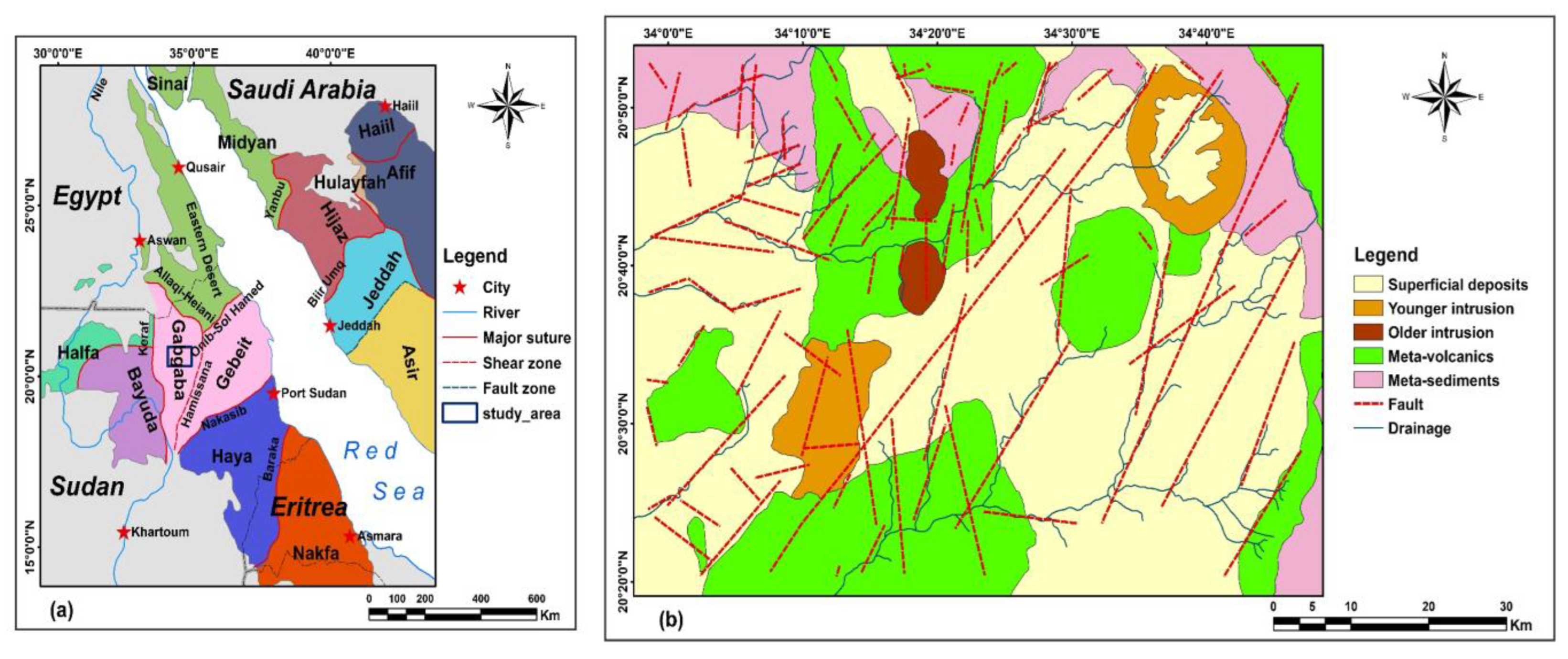
2. Study Area
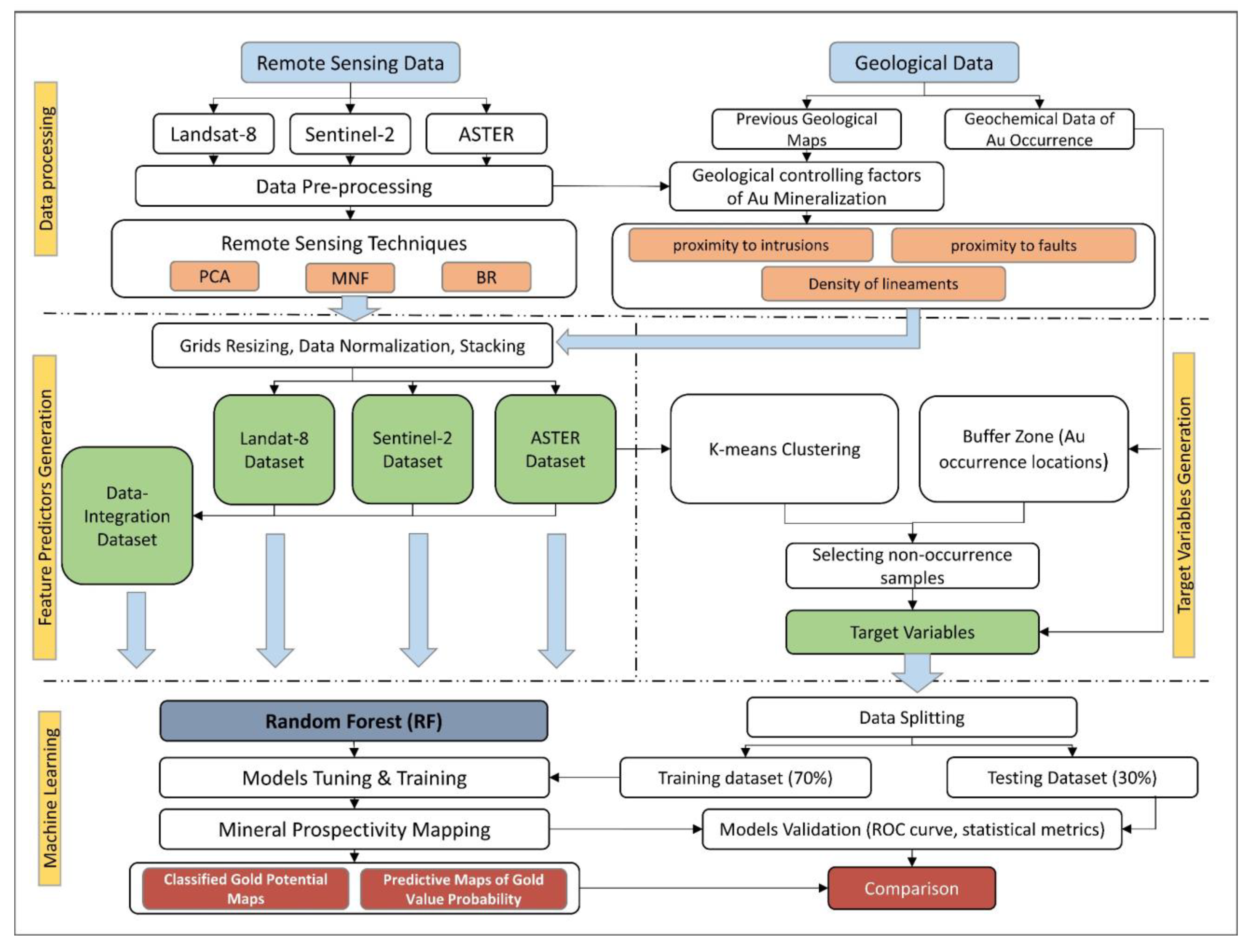
3. Materials and Methods
3.1. Data and Data-Preprocessing
3.2. Random Forest (RF)
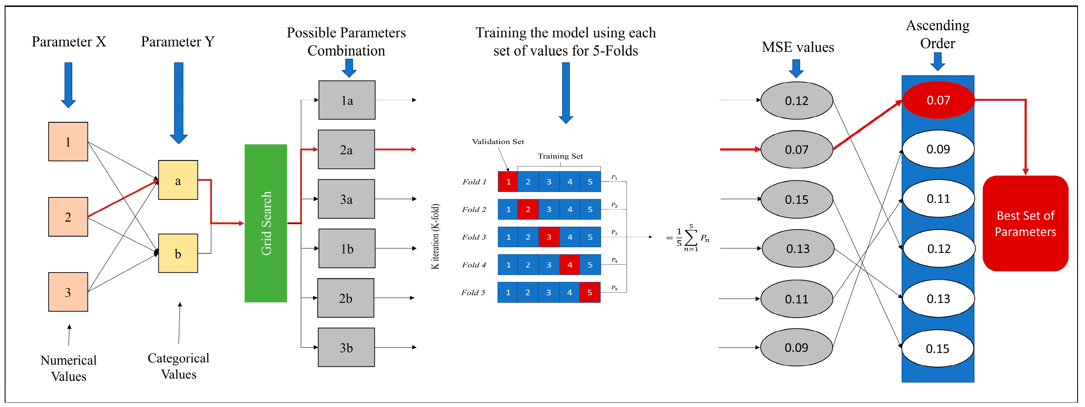
3.3. Induction of RF Predictive Model
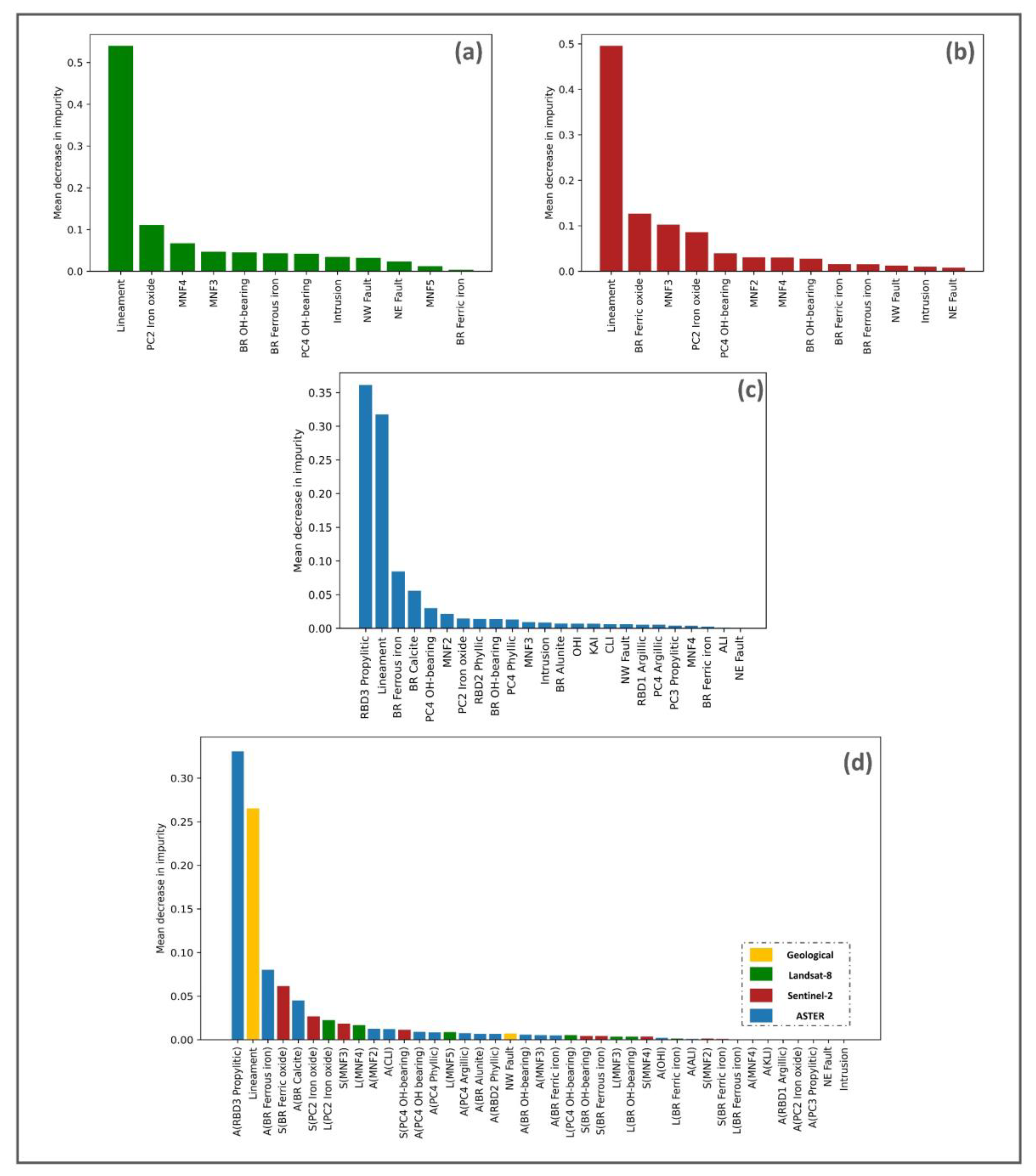
3.4. Predictor Variables
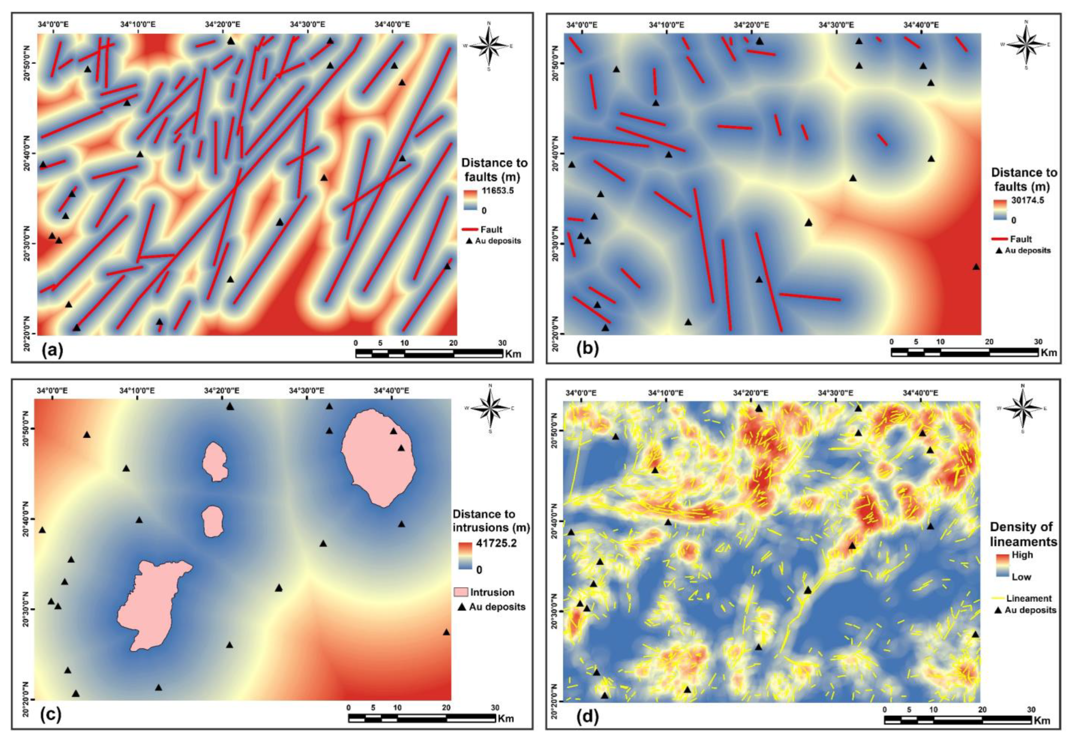
3.4.1. Geological-Based Predictor Maps
3.4.2. Remote Sensing-Based Predictor Maps
3.4.3. Data Preparation
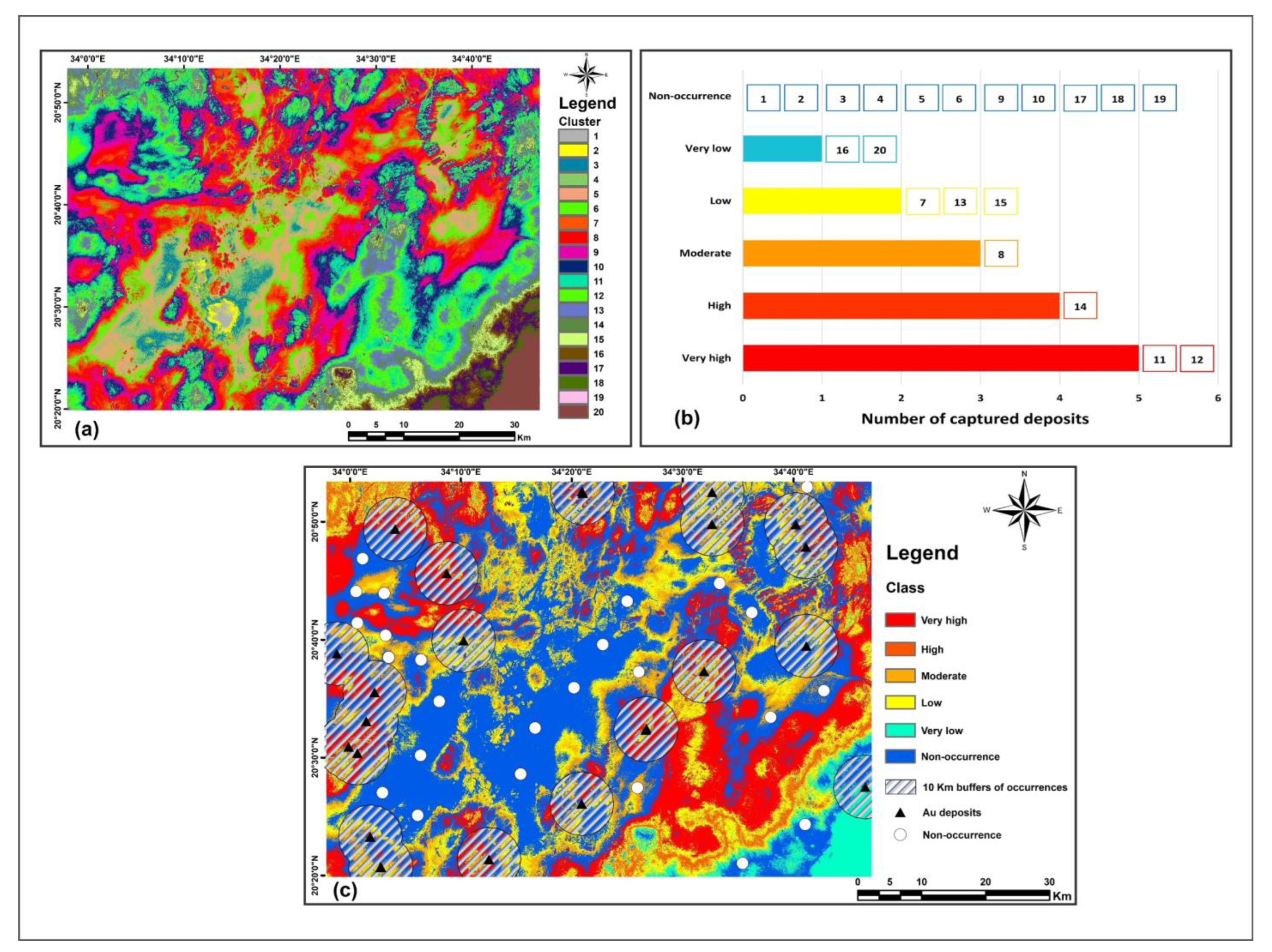
3.5. Target Variable
- The number of non-occurrence samples must be equal to the number of mineral occurrences.
- Non-occurrence samples should be spatially distributed randomly.
- The selection of non-occurrence locations should be distal from any known gold occurrences. Here, we applied a 10 km buffer zone around known occurrences.
3.6. Model Assessment
4. Results
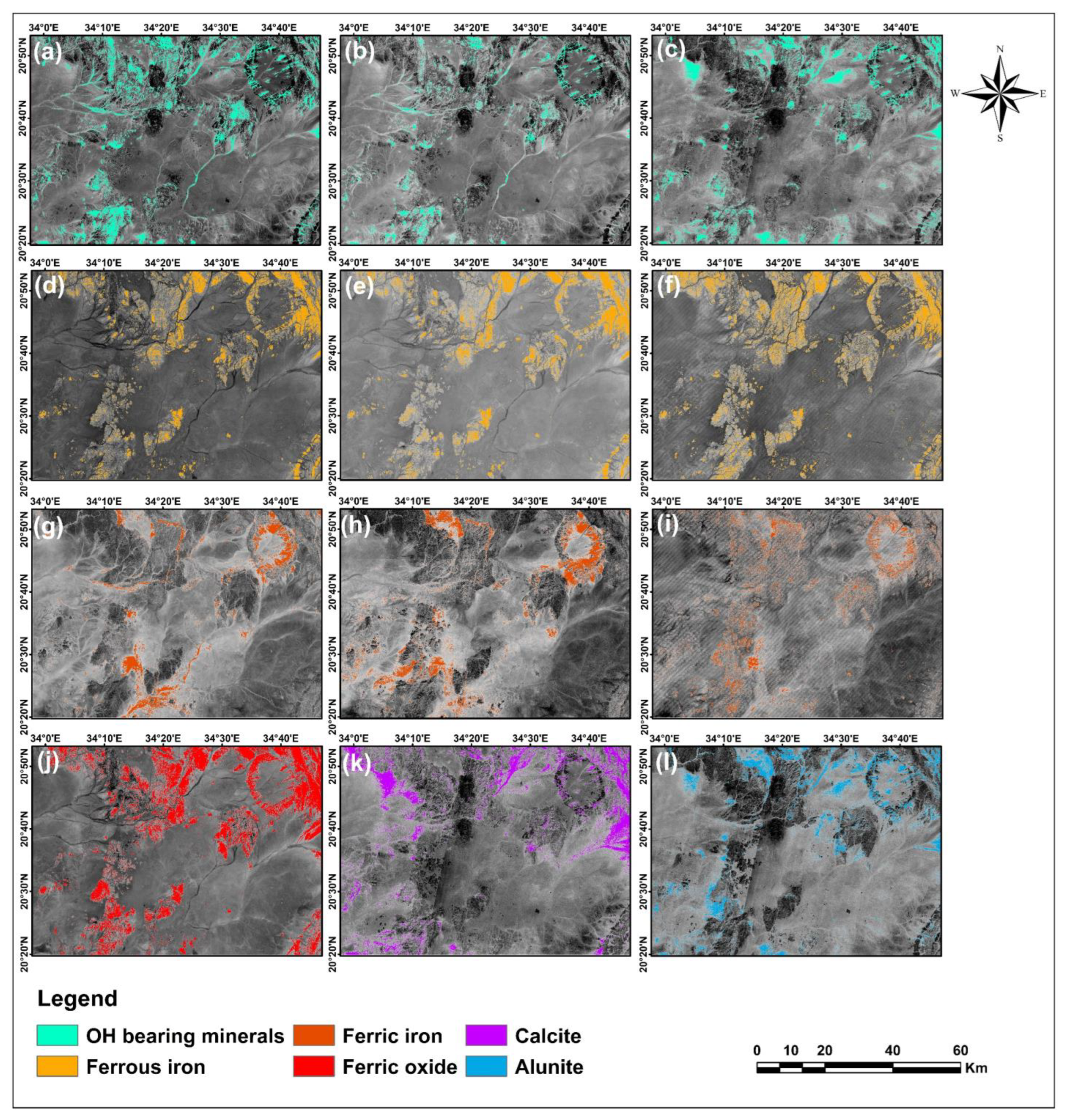
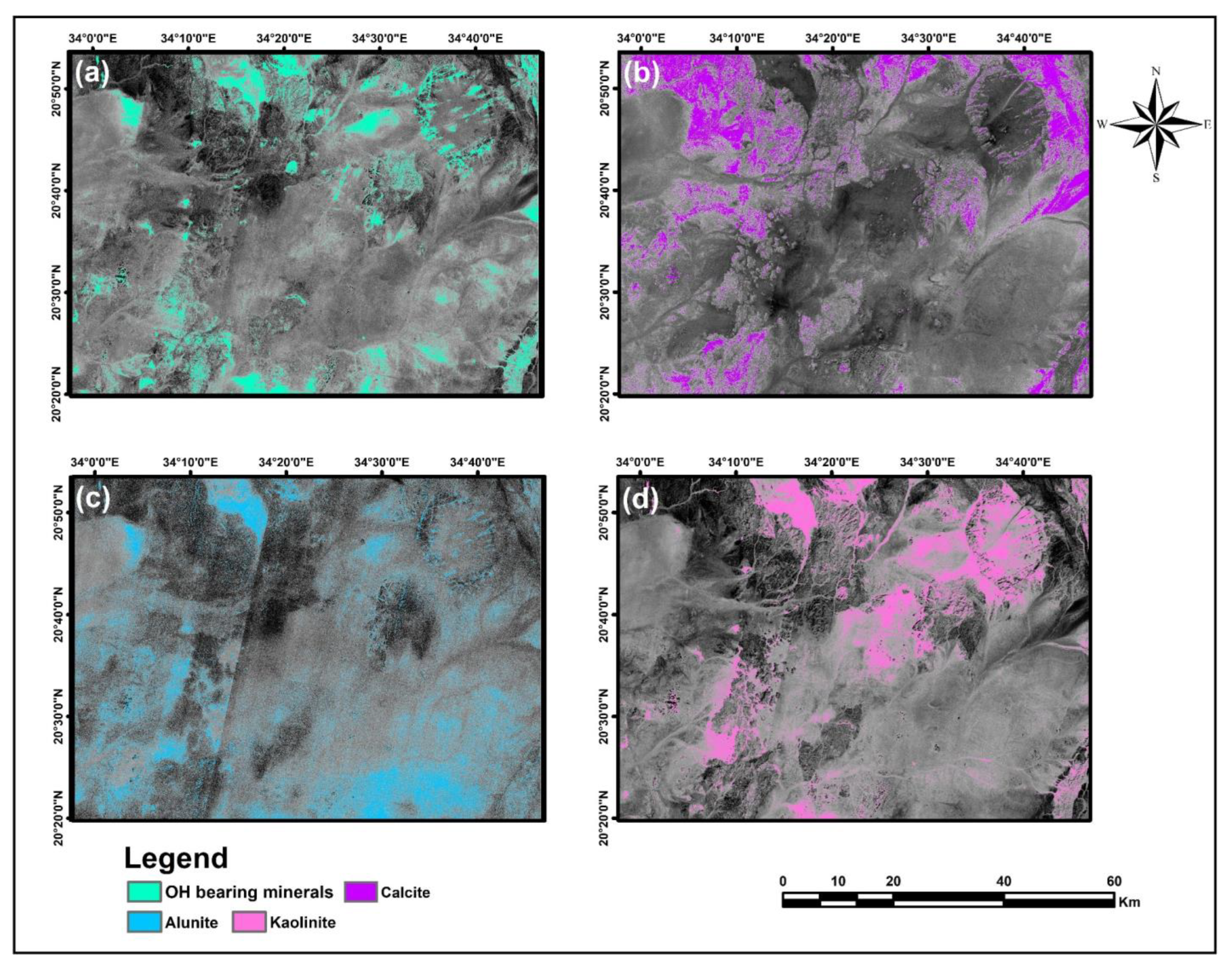
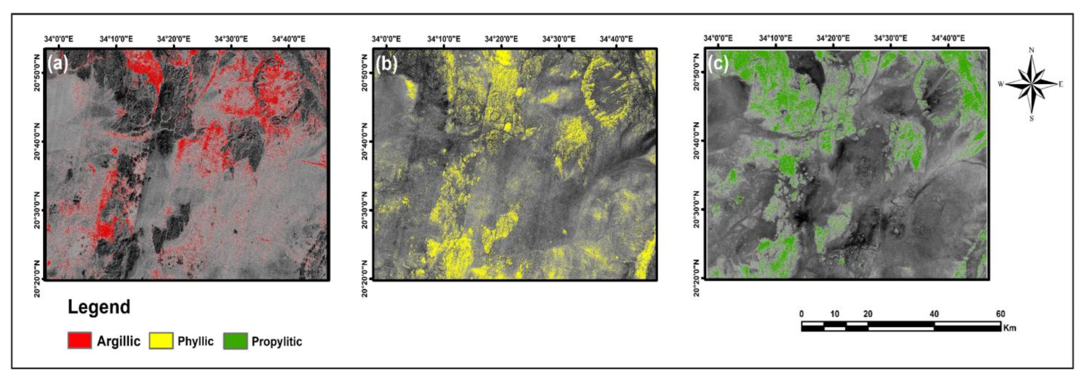
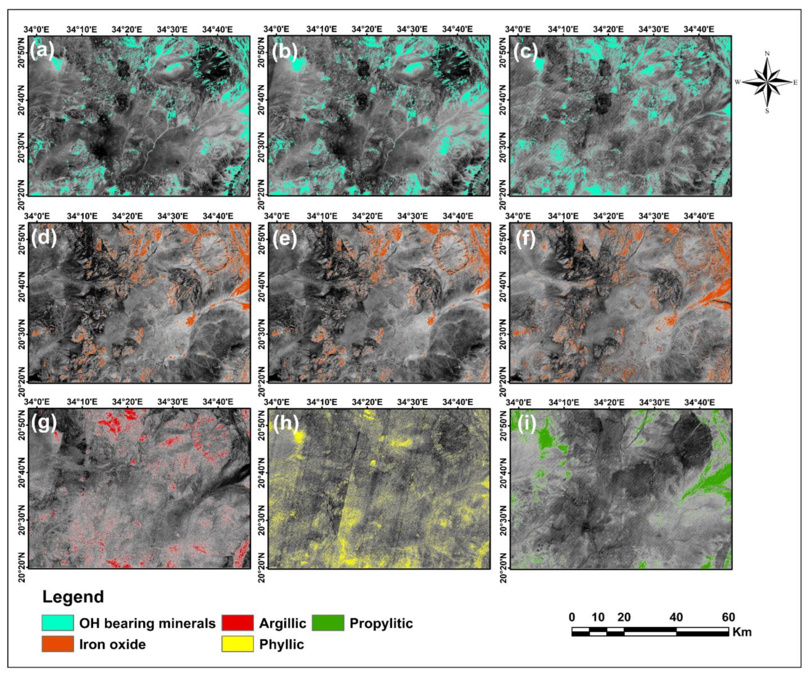
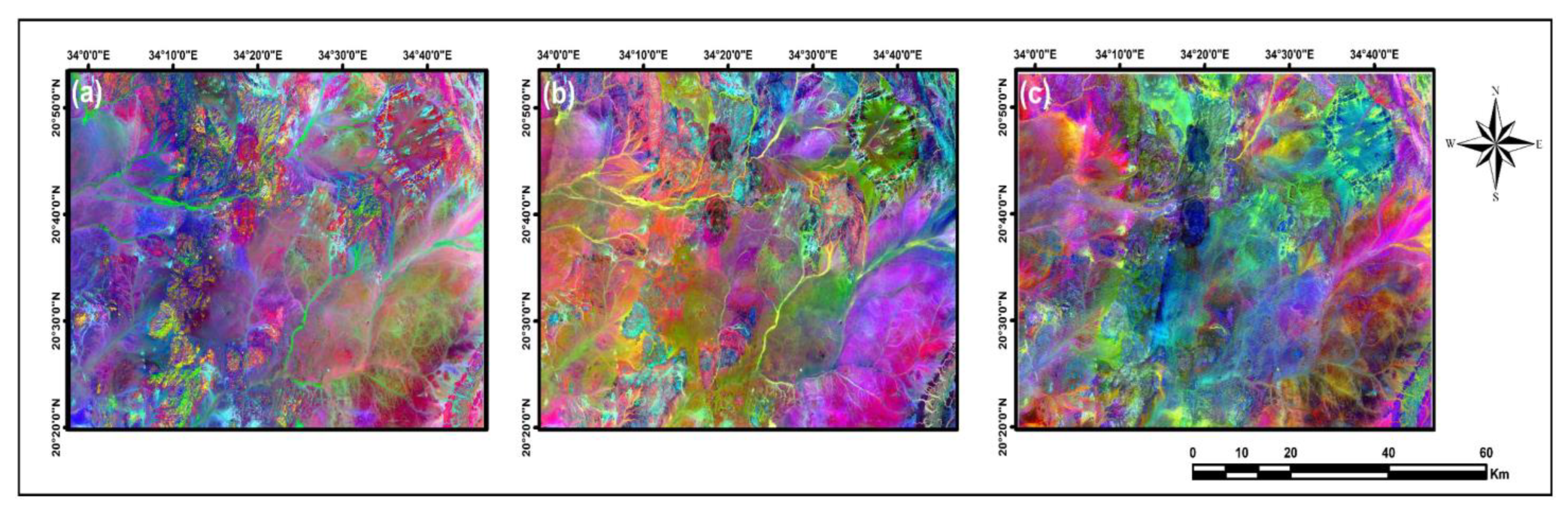
4.1. Generating Remote Sensing-Based Predictor Maps
4.2. Generating Target Variable Using K-Means Clustering
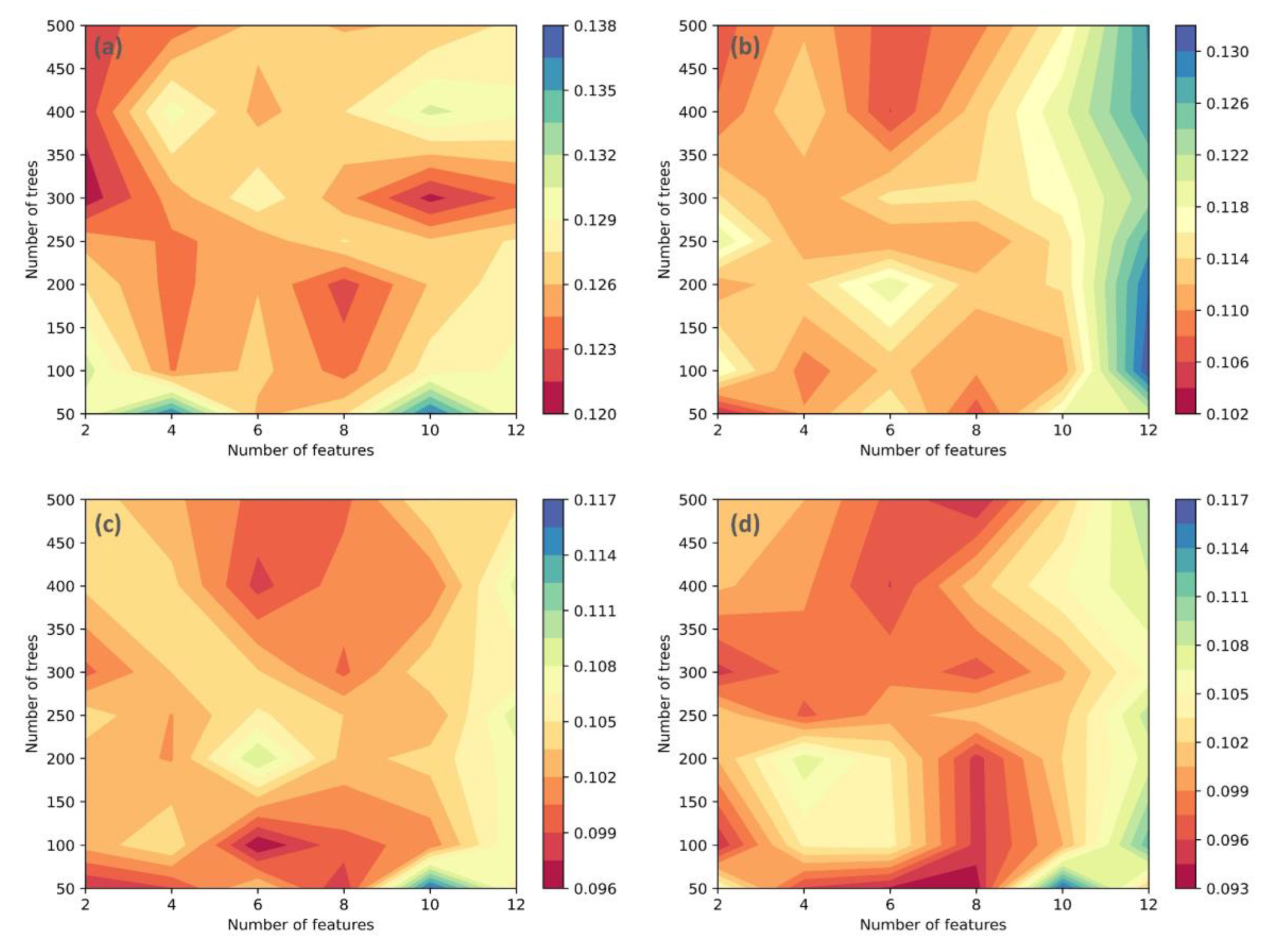
4.3. Sensitivity of RF Predictive Model to Parameter Tuning
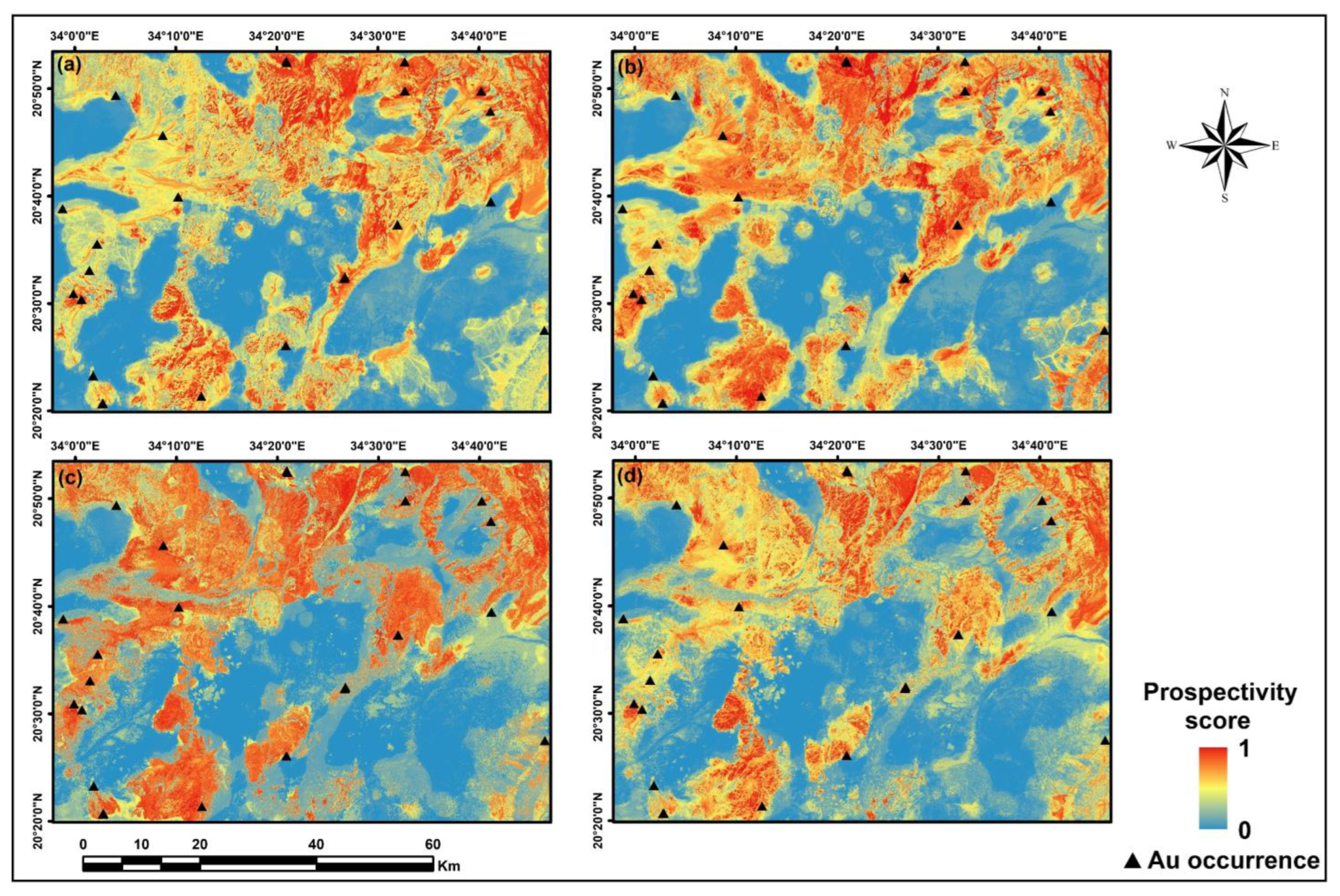
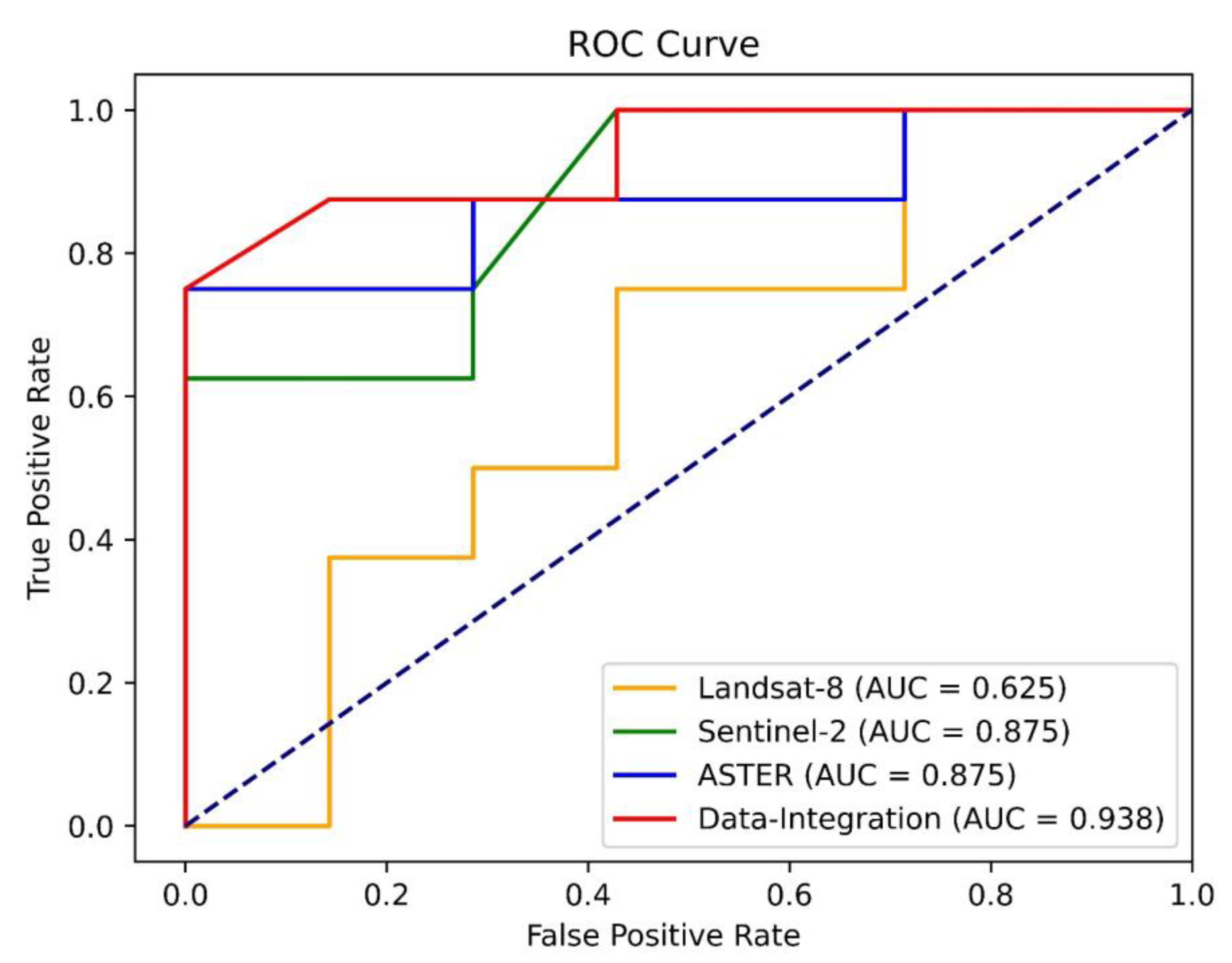
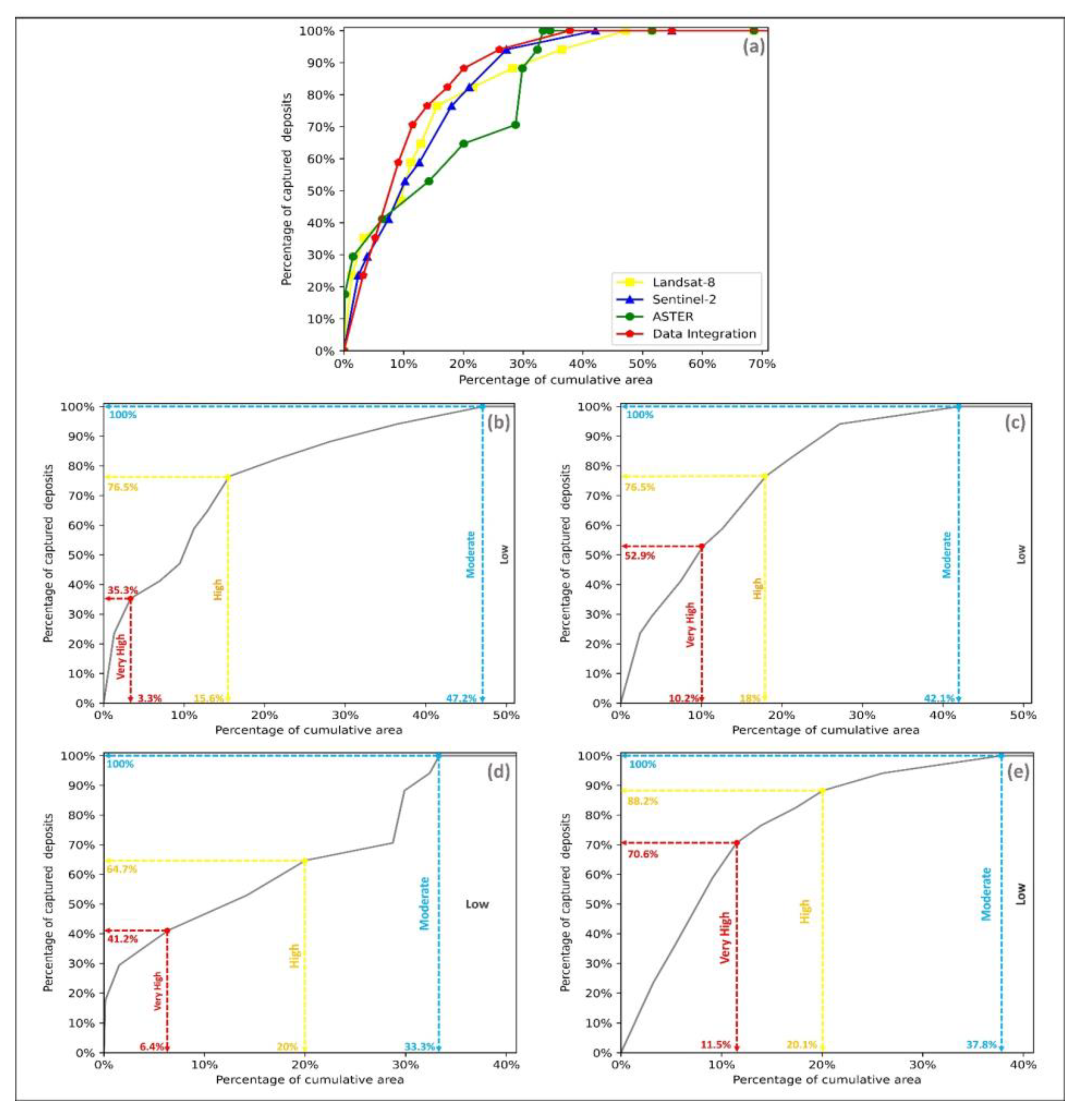
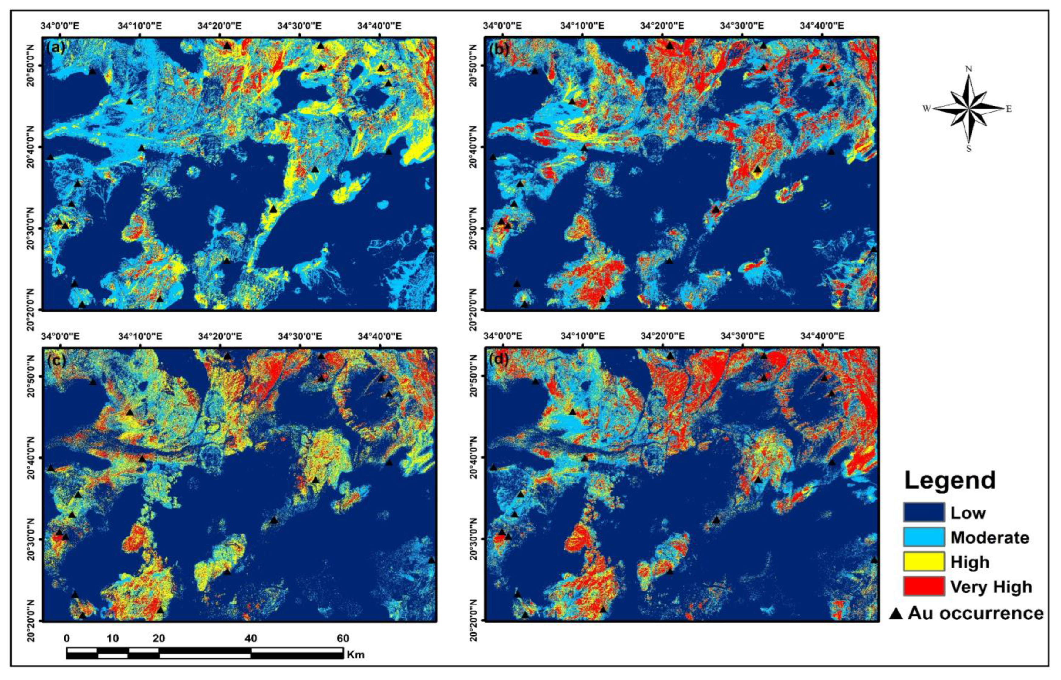
4.4. Comparison of Various Datasets Performance
5. Discussion
6. Conclusions
Author Contributions
Funding
Data Availability Statement
Acknowledgments
Conflicts of Interest
References
- Arndt, N.T.; Fontboté, L.; Hedenquist, J.W.; Kesler, S.E.; Thompson, J.F.; Wood, D.G. Future global mineral resources. Geochem. Perspect. 2017, 6, 1–171. [Google Scholar] [CrossRef] [Green Version]
- Wang, K.; Zheng, X.; Wang, G.; Liu, D.; Cui, N. A Multi-Model Ensemble Approach for Gold Mineral Prospectivity Mapping: A Case Study on the Beishan Region, Western China. Minerals 2020, 10, 1126. [Google Scholar] [CrossRef]
- Sun, T.; Li, H.; Wu, K.; Chen, F.; Zhu, Z.; Hu, Z. Data-Driven Predictive Modelling of Mineral Prospectivity Using Machine Learning and Deep Learning Methods: A Case Study from Southern Jiangxi Province, China. Minerals 2020, 10, 102. [Google Scholar] [CrossRef] [Green Version]
- Carranza, E.J.M.; Laborte, A.G. Data-driven predictive mapping of gold prospectivity, Baguio district, Philippines: Application of Random Forests algorithm. Ore Geol. Rev. 2015, 71, 777–787. [Google Scholar] [CrossRef]
- Porwal, A.; Carranza, E.J.M. Introduction to the Special Issue: GIS-based mineral potential modelling and geological data analyses for mineral exploration. Ore Geol. Rev. 2015, 71, 477–483. [Google Scholar] [CrossRef]
- Carranza, E.J.M.; Hale, M.; Faassen, C. Selection of coherent deposit-type locations and their application in data-driven mineral prospectivity mapping. Ore Geol. Rev. 2008, 33, 536–558. [Google Scholar] [CrossRef]
- Rodriguez-Galiano, V.; Sanchez-Castillo, M.; Chica-Olmo, M.; Chica-Rivas, M. Machine learning predictive models for mineral prospectivity: An evaluation of neural networks, random forest, regression trees and support vector machines. Ore Geol. Rev. 2015, 71, 804–818. [Google Scholar] [CrossRef]
- Sun, T.; Chen, F.; Zhong, L.; Liu, W.; Wang, Y. GIS-based mineral prospectivity mapping using machine learning methods: A case study from Tongling ore district, eastern China. Ore Geol. Rev. 2019, 109, 26–49. [Google Scholar] [CrossRef]
- Yousefi, M.; Nykänen, V. Introduction to the special issue: GIS-based mineral potential targeting. J. Afr. Earth Sci. 2017, 128, 1–4. [Google Scholar] [CrossRef]
- Cheng, Q.M.; Agterberg, F.P. Fuzzy weights of evidence method and its application in mineral potential mapping. Nat. Resour. Res. 1999, 8, 27–35. [Google Scholar] [CrossRef]
- Abedi, M.; Norouzi, G.-H.; Fathianpour, N. Fuzzy outranking approach: A knowledge-driven method for mineral prospectivity mapping. Int. J. Appl. Earth Obs. Geoinf. 2013, 21, 556–567. [Google Scholar] [CrossRef]
- Yousefi, M.; Nykänen, V. Data-driven logistic-based weighting of geochemical and geological evidence layers in mineral prospectivity mapping. J. Geochem. Explor. 2016, 164, 94–106. [Google Scholar] [CrossRef]
- Ghezelbash, R.; Maghsoudi, A.; Bigdeli, A.; Carranza, E.J.M. Regional-Scale Mineral Prospectivity Mapping: Support Vector Machines and an Improved Data-Driven Multi-criteria Decision-Making Technique. Nat. Resour. Res. 2021, 30, 1977–2005. [Google Scholar] [CrossRef]
- Harris, J.R.; Grunsky, E.; Behnia, P.; Corrigan, D. Data- and knowledge-driven mineral prospectivity maps for Canada’s North. Ore Geol. Rev. 2015, 71, 788–803. [Google Scholar] [CrossRef]
- Abdelkareem, M.; Al-Arifi, N. Synergy of Remote Sensing Data for Exploring Hydrothermal Mineral Resources Using GIS-Based Fuzzy Logic Approach. Remote Sens. 2021, 13, 4492. [Google Scholar] [CrossRef]
- Rowan, L.C.; Mars, J.C. Lithologic mapping in the Mountain Pass, California area using advanced spaceborne thermal emission and reflection radiometer (ASTER) data. Remote Sens. Environ. 2003, 84, 350–366. [Google Scholar] [CrossRef]
- Pazand, K.; Pazand, K. Identification of hydrothermal alteration minerals for exploring porphyry copper deposit using ASTER data: A case study of Varzaghan area, NW Iran. Geol. Ecol. Landsc. 2020, 6, 217–223. [Google Scholar] [CrossRef]
- Pour, A.B.; Hashim, M. Identification of hydrothermal alteration minerals for exploring of porphyry copper deposit using ASTER data, SE Iran. J. Asian Earth Sci. 2011, 42, 1309–1323. [Google Scholar] [CrossRef]
- Guha, A.; Mondal, S.; Chatterjee, S.; Kumar, K.V. Airborne imaging spectroscopy of igneous layered complex and their mapping using different spectral enhancement conjugated support vector machine models. Geocarto Int. 2020, 37, 349–365. [Google Scholar] [CrossRef]
- Rao, D.A.; Guha, A. Potential Utility of Spectral Angle Mapper and Spectral Information Divergence Methods for mapping lower Vindhyan Rocks and Their Accuracy Assessment with Respect to Conventional Lithological Map in Jharkhand, India. J. Indian Soc. Remote 2018, 46, 737–747. [Google Scholar] [CrossRef]
- Rani, N.; Mandla, V.R.; Singh, T. Spatial distribution of altered minerals in the Gadag Schist Belt (GSB) of Karnataka, Southern India using hyperspectral remote sensing data. Geocarto Int. 2016, 32, 225–237. [Google Scholar] [CrossRef]
- Rani, N.; Mandla, V.R.; Singh, T. Evaluation of atmospheric corrections on hyperspectral data with special reference to mineral mapping. Geosci. Front. 2017, 8, 797–808. [Google Scholar] [CrossRef] [Green Version]
- Noori, L.; Pour, A.; Askari, G.; Taghipour, N.; Pradhan, B.; Lee, C.-W.; Honarmand, M. Comparison of Different Algorithms to Map Hydrothermal Alteration Zones Using ASTER Remote Sensing Data for Polymetallic Vein-Type Ore Exploration: Toroud–Chahshirin Magmatic Belt (TCMB), North Iran. Remote Sens. 2019, 11, 495. [Google Scholar] [CrossRef] [Green Version]
- Pour, A.B.; Hashim, M. Identifying areas of high economic-potential copper mineralization using ASTER data in the Urumieh–Dokhtar Volcanic Belt, Iran. Adv. Space Res. 2012, 49, 753–769. [Google Scholar] [CrossRef]
- Pour, A.B.; Hashim, M.; Makoundi, C.; Zaw, K. Structural Mapping of the Bentong-Raub Suture Zone Using PALSAR Remote Sensing Data, Peninsular Malaysia: Implications for Sediment-hosted/Orogenic Gold Mineral Systems Exploration. Resour. Geol. 2016, 66, 368–385. [Google Scholar] [CrossRef]
- Pour, A.B.; Hashim, M.; Park, Y. Application of ASTER SWIR bands in mapping anomaly pixels for Antarctic geological mapping. J. Phys. Conf. Ser. 2017, 852, 012025. [Google Scholar] [CrossRef] [Green Version]
- Pour, A.B.; Park, Y.; Park, T.-Y.S.; Hong, J.K.; Hashim, M.; Woo, J.; Ayoobi, I. Regional geology mapping using satellite-based remote sensing approach in Northern Victoria Land, Antarctica. Polar Sci. 2018, 16, 23–46. [Google Scholar] [CrossRef]
- Son, Y.-S.; Lee, G.; Lee, B.H.; Kim, N.; Koh, S.-M.; Kim, K.-E.; Cho, S.-J. Application of ASTER Data for Differentiating Carbonate Minerals and Evaluating MgO Content of Magnesite in the Jiao-Liao-Ji Belt, North China Craton. Remote Sens. 2022, 14, 181. [Google Scholar] [CrossRef]
- Bahrami, Y.; Hassani, H.; Maghsoudi, A. Investigating the capabilities of multispectral remote sensors data to map alteration zones in the Abhar area, NW Iran. Geosyst. Eng. 2018, 24, 18–30. [Google Scholar] [CrossRef]
- Fereydooni, H.; Mojeddifar, S. A directed matched filtering algorithm (DMF) for discriminating hydrothermal alteration zones using the ASTER remote sensing data. Int. J. Appl. Earth Obs. Geoinf. 2017, 61, 1–13. [Google Scholar] [CrossRef]
- Chen, Q.; Zhao, Z.-F.; Xia, J.-S.; Zhao, X.; Yang, H.-Y.; Zhang, X.-L. Improving the accuracy of hydrothermal alteration mapping based on image fusion of ASTER and Sentinel-2A data: A case study of Pulang Cu deposit, Southwest China. Geocarto Int. 2022, 1–26. [Google Scholar] [CrossRef]
- Joly, A.; Porwal, A.; McCuaig, T.C.; Chudasama, B.; Dentith, M.C.; Aitken, A.R.A. Mineral systems approach applied to GIS-based 2D-prospectivity modelling of geological regions: Insights from Western Australia. Ore Geol. Rev. 2015, 71, 673–702. [Google Scholar] [CrossRef]
- Carranza, E.J.M. Natural Resources Research Publications on Geochemical Anomaly and Mineral Potential Mapping, and Introduction to the Special Issue of Papers in These Fields. Nat. Resour. Res. 2017, 26, 379–410. [Google Scholar] [CrossRef]
- Carranza, E.J.M.; Laborte, A.G. Random forest predictive modeling of mineral prospectivity with small number of prospects and data with missing values in Abra (Philippines). Comput. Geosci. 2015, 74, 60–70. [Google Scholar] [CrossRef]
- Zuo, R.; Carranza, E.J.M. Support vector machine: A tool for mapping mineral prospectivity. Comput. Geosci. 2011, 37, 1967–1975. [Google Scholar] [CrossRef]
- Brown, W.M.; Gedeon, T.D.; Groves, D.I.; Barnes, R.G. Artifcial neural network: A new method for mineral prospectivity mapping. Aust. J. Earth Sci. 2000, 47, 757–770. [Google Scholar] [CrossRef]
- Xi, Y.; Mohamed Taha, A.M.; Hu, A.; Liu, X. Accuracy comparison of various remote sensing data in lithological classification based on random forest algorithm. Geocarto Int. 2022, 1–29. [Google Scholar] [CrossRef]
- Mansouri, E.; Feizi, F.; Jafari Rad, A.; Arian, M. Remote-sensing data processing with the multivariate regression analysis method for iron mineral resource potential mapping: A case study in the Sarvian area, central Iran. Solid Earth 2018, 9, 373–384. [Google Scholar] [CrossRef] [Green Version]
- Bolouki, S.M.; Ramazi, H.R.; Maghsoudi, A.; Beiranvand Pour, A.; Sohrabi, G. A Remote Sensing-Based Application of Bayesian Networks for Epithermal Gold Potential Mapping in Ahar-Arasbaran Area, NW Iran. Remote Sens. 2019, 12, 105. [Google Scholar] [CrossRef] [Green Version]
- Rodriguez-Galiano, V.F.; Chica-Olmo, M.; Chica-Rivas, M. Predictive modelling of gold potential with the integration of multisource information based on random forest: A case study on the Rodalquilar area, Southern Spain. Int. J. Geogr. Inf. Sci. 2014, 28, 1336–1354. [Google Scholar] [CrossRef]
- Gaboury, D.; Nabil, H.; Ennaciri, A.; Maacha, L. Structural setting and fluid composition of gold mineralization along the central segment of the Keraf suture, Neoproterozoic Nubian Shield, Sudan: Implications for the source of gold. Int. Geol. Rev. 2020, 64, 45–71. [Google Scholar] [CrossRef]
- Mohamed, M.T.A.; Al-Naimi, L.S.; Mgbeojedo, T.I.; Agoha, C.C. Geological mapping and mineral prospectivity using remote sensing and GIS in parts of Hamissana, Northeast Sudan. J. Pet. Explor. Prod. 2021, 11, 1123–1138. [Google Scholar] [CrossRef]
- Bierlein, F.; Reynolds, N.; Arne, D.; Bargmann, C.; McKeag, S.; Bullen, W.; Al-Athbah, H.; McKnight, S.; Maas, R. Petrogenesis of a Neoproterozoic magmatic arc hosting porphyry Cu-Au mineralization at Jebel Ohier in the Gebeit Terrane, NE Sudan. Ore Geol. Rev. 2016, 79, 133–154. [Google Scholar] [CrossRef]
- Zeinelabdein, K.A.E.; Nadi, A.H.H.E. The use of Landsat 8 OLI image for the delineation of gossanic ridges in the Red Sea Hills of NE Sudan. Am. J. Earth Sci. 2014, 1, 62–67. [Google Scholar]
- Sasmaz, A. The Atbara porphyry gold–copper systems in the Red Sea Hills, Neoproterozoic Arabian–Nubian Shield, NE Sudan. J. Geochem. Explor. 2020, 214, 106539. [Google Scholar] [CrossRef]
- El Khidir, S.O.; Babikir, I.A. Digital image processing and geospatial analysis of landsat 7 ETM+ for mineral exploration, Abidiya area, North Sudan. Int. J. Geomat. Geosci. 2013, 3, 645–658. [Google Scholar]
- Ali, A.; Pour, A. Lithological mapping and hydrothermal alteration using Landsat 8 data: A case study in ariab mining district, red sea hills, Sudan. Int. J. Basic Appl. Sci. 2014, 3, 199–208. [Google Scholar] [CrossRef]
- Breiman, L. Random Forests. Mach. Learn. 2001, 45, 5–32. [Google Scholar] [CrossRef] [Green Version]
- Breiman, L. bagging predictors. Mach. Learn. 1996, 24, 123–140. [Google Scholar] [CrossRef] [Green Version]
- Breiman, L.; Friedman, J.; Olshen, R.; Stone, C. Classification and Regression Trees; Wadsworth & Brooks; Cole Statistics/Probability Series; Chapman & Hall: London, UK, 1984. [Google Scholar]
- Belgiu, M.; Drăguţ, L. Random forest in remote sensing: A review of applications and future directions. ISPRS J. Photogramm. Remote Sens. 2016, 114, 24–31. [Google Scholar] [CrossRef]
- Shah, S.H.; Angel, Y.; Houborg, R.; Ali, S.; McCabe, M.F. A Random Forest Machine Learning Approach for the Retrieval of Leaf Chlorophyll Content in Wheat. Remote Sens. 2019, 11, 920. [Google Scholar] [CrossRef] [Green Version]
- Kulkarni, A.D.; Lowe, B. Random forest algorithm for land cover classification. Int. J. Recent Innov. Trends Comput. Commun. 2016, 4, 58–63. [Google Scholar]
- Pal, M. Random forest classifier for remote sensing classification. Int. J. Remote Sens. 2005, 26, 217–222. [Google Scholar] [CrossRef]
- Maepa, F.; Smith, R.S.; Tessema, A. Support vector machine and artificial neural network modelling of orogenic gold prospectivity mapping in the Swayze greenstone belt, Ontario, Canada. Ore Geol. Rev. 2021, 130, 103968. [Google Scholar] [CrossRef]
- Zeinelabdein, K.E.; Albiely, A. Ratio image processing techniques: A prospecting tool for mineral deposits, Red Sea Hills, NE Sudan. Int. Arch. Photogramm. Remote Sens. Spat. Inf. Sci. 2008, 37, 1295–1298. [Google Scholar]
- Abdullah, A.; Nassr, S.; Ghaleeb, A. Remote Sensing and Geographic Information System for Fault Segments Mapping a Study from Taiz Area, Yemen. J. Geol. Res. 2013, 2013, 201757. [Google Scholar] [CrossRef] [Green Version]
- Adiria, Z.; Hartia, A.E.; Jelloulia, A.; Lhissoua, R.; Maachab, L.; Azmib, M.; Zouhairb, M.; Bachaouia, E.M. Comparison of Landsat-8, ASTER and Sentinel 1 satellite remote sensing data in automatic lineaments extraction: A case study of Sidi Flah Bouskour inlier, Moroccan Anti Atlas. Adv. Space Res. 2017, 60, 2355–2367. [Google Scholar] [CrossRef]
- Pour, A.B.; Hashim, M. ASTER, ALI and Hyperion sensors data for lithological mapping and ore minerals exploration. SpringerPlus 2014, 3, 130. [Google Scholar] [CrossRef] [Green Version]
- Li, N. Textural and Rule-Based Lithological Classification of Remote Sensing Data, and Geological Mapping in Southwestern Prieska Sub-Basin, Transvaal Supergroup, South Africa. Ph.D. Thesis, LMU, München, Germany, 2010. [Google Scholar]
- Zhang, T.; Yi, G.; Li, H.; Wang, Z.; Tang, J.; Zhong, K.; Li, Y.; Wang, Q.; Bie, X. Integrating Data of ASTER and Landsat-8 OLI (AO) for Hydrothermal Alteration Mineral Mapping in Duolong Porphyry Cu-Au Deposit, Tibetan Plateau, China. Remote Sens. 2016, 8, 890. [Google Scholar] [CrossRef] [Green Version]
- Sabins, F.F. Remote sensing for mineral exploration. Ore Geol. Rev. 1999, 14, 157–183. [Google Scholar] [CrossRef]
- Inzana, J.; Kusky, T.; Higgs, G.; Tucker, R. Supervised classifications of Landsat TM band ratio images and Landsat TM band ratio image with radar for geological interpretations of central Madagascar. J. Afr. Earth Sci. 2003, 37, 59–72. [Google Scholar] [CrossRef]
- Ninomiya, Y. Lithologic Mapping with Multispectral ASTER TIR and SWIR Data; SPIE: Bellingham, WA, USA, 2004. [Google Scholar]
- Ninomiya, Y.; Fu, B.; Cudahy, T.J. Detecting lithology with Advanced Spaceborne Thermal Emission and Reflection Radiometer (ASTER) multispectral thermal infrared “radiance-at-sensor” data. Remote Sens. Environ. 2005, 99, 127–139. [Google Scholar] [CrossRef]
- Rajan Girija, R.; Mayappan, S. Mapping of mineral resources and lithological units: A review of remote sensing techniques. Int. J. Image Data Fusion 2019, 10, 79–106. [Google Scholar] [CrossRef]
- Ninomiya, Y. A stabilized vegetation index and several mineralogic indices defined for ASTER VNIR and SWIR data. In Proceedings of the IGARSS 2003, 2003 IEEE International Geoscience and Remote Sensing Symposium, Proceedings (IEEE Cat. No.03CH37477), Toulouse, France, 21–25 July 2003; pp. 1552–1554. [Google Scholar]
- van der Meer, F.D.; van der Werff, H.M.A.; van Ruitenbeek, F.J.A. Potential of ESA’s Sentinel-2 for geological applications. Remote Sens. Environ. 2014, 148, 124–133. [Google Scholar] [CrossRef]
- Ge, W.; Cheng, Q.; Jing, L.; Wang, F.; Zhao, M.; Ding, H. Assessment of the Capability of Sentinel-2 Imagery for Iron-Bearing Minerals Mapping: A Case Study in the Cuprite Area, Nevada. Remote Sens. 2020, 12, 3028. [Google Scholar] [CrossRef]
- Timkin, T.; Abedini, M.; Ziaii, M.; Ghasemi, M.R. Geochemical and Hydrothermal Alteration Patterns of the Abrisham-Rud Porphyry Copper District, Semnan Province, Iran. Minerals 2022, 12, 103. [Google Scholar] [CrossRef]
- Crosta, A.; De Souza Filho, C.; Azevedo, F.; Brodie, C. Targeting key alteration minerals in epithermal deposits in Patagonia, Argentina, using ASTER imagery and principal component analysis. Int. J. Remote Sens. 2003, 24, 4233–4240. [Google Scholar] [CrossRef]
- Ourhzif, Z.; Algouti, A.; Algouti, A.; Hadach, F. Lithological Mapping Using Landsat 8 Oli and Aster Multispectral Data in Imini-Ounilla District South High Atlas of Marrakech. Int. Arch. Photogramm. Remote Sens. Spat. Inf. Sci. 2019, XLII-2/W13, 1255–1262. [Google Scholar] [CrossRef] [Green Version]
- Saljoughi, B.S.; Hezarkhani, A. A comparative analysis of artificial neural network (ANN), wavelet neural network (WNN), and support vector machine (SVM) data-driven models to mineral potential mapping for copper mineralizations in the Shahr-e-Babak region, Kerman, Iran. Appl. Geomat. 2018, 10, 229–256. [Google Scholar] [CrossRef]
- Torppa, J.; Nykänen, V.; Molnár, F. Unsupervised clustering and empirical fuzzy memberships for mineral prospectivity modelling. Ore Geol. Rev. 2019, 107, 58–71. [Google Scholar] [CrossRef]
- Bachri, I.; Hakdaoui, M.; Raji, M.; Teodoro, A.C.; Benbouziane, A. Machine Learning Algorithms for Automatic Lithological Mapping Using Remote Sensing Data: A Case Study from Souk Arbaa Sahel, Sidi Ifni Inlier, Western Anti-Atlas, Morocco. ISPRS Int. J. Geo-Inf. 2019, 8, 248. [Google Scholar] [CrossRef] [Green Version]
- Cracknell, M.J.; Reading, A.M. Geological mapping using remote sensing data: A comparison of five machine learning algorithms, their response to variations in the spatial distribution of training data and the use of explicit spatial information. Comput. Geosci. 2014, 63, 22–33. [Google Scholar] [CrossRef] [Green Version]
- Heydari, S.S.; Mountrakis, G. Effect of classifier selection, reference sample size, reference class distribution and scene heterogeneity in per-pixel classification accuracy using 26 Landsat sites. Remote Sens. Environ. 2018, 204, 648–658. [Google Scholar] [CrossRef]
- Barsi, Á.; Kugler, Z.; László, I.; Szabó, G.; Abdulmutalib, H.M. Accuracy Dimensions in Remote Sensing. Int. Arch. Photogramm. Remote Sens. Spat. Inf. Sci. 2018, XLII-3, 61–67. [Google Scholar] [CrossRef]
- Agterberg, F.P.; Bonham-Carter, G.F. Measuring the Performance of Mineral-Potential Maps. Nat. Resour. Res. 2005, 14, 1–17. [Google Scholar] [CrossRef]
- Landgrebe, T.C.W.; Paclik, P. The ROC skeleton for multiclass ROC estimation. Pattern Recognit. Lett. 2010, 31, 949–958. [Google Scholar] [CrossRef]
- Bradley, A.P. The use of the area under the ROC curve in the evaluation of machine learning algorithms. Pattern Recognit. 1997, 30, 1145–1159. [Google Scholar] [CrossRef] [Green Version]
- Hua, B.; Xua, Y.; Wana, B.; Wua, X.; Yi, G. Hydrothermally altered mineral mapping using synthetic application of Sentinel-2A MSI, ASTER and Hyperion data in the Duolong area, Tibetan Plateau, China. Ore Geol. Rev. 2018, 101, 384–397. [Google Scholar] [CrossRef]
- Ge, W.; Cheng, Q.; Jing, L.; Armenakis, C.; Ding, H. Lithological discrimination using ASTER and Sentinel-2A in the Shibanjing ophiolite complex of Beishan orogenic in Inner Mongolia, China. Adv. Space Res. 2018, 62, 1702–1716. [Google Scholar] [CrossRef]
- Ge, W.; Cheng, Q.; Tang, Y.; Jing, L.; Gao, C. Lithological Classification Using Sentinel-2A Data in the Shibanjing Ophiolite Complex in Inner Mongolia, China. Remote Sens. 2018, 10, 638. [Google Scholar] [CrossRef]


| Satellite | Bands | Wavelength (µm) | Spatial Resolution (m) | Scene ID | Date and Time of Acquisition | Other Info |
|---|---|---|---|---|---|---|
| Landsat-8 | Band 1-(coastal/aerosol) | 0.435–0.451 | 30 | LC81730462021360LGN00 | 26 December 2021 08:08:23 | Path = 173 Row = 46 |
| Band 2-Blue | 0.452–0.512 | 30 | ||||
| Band 3-Green | 0.533–0.590 | 30 | ||||
| Band 4-Red | 0.636–0.673 | 30 | ||||
| Band 5-(NIR) | 0.851–0.879 | 30 | ||||
| Band 6-(SWIR) 1 | 1.566–1.651 | 30 | ||||
| Band 7-(SWIR) 2 | 2.107–2.294 | 30 | ||||
| Band 8-Panchromatic | 0.503–0.676 | 15 | ||||
| Band 9-Cirrus | 1.363–1.384 | 30 | ||||
| Band 10-(TIRS) 1 | 10.60–11.19 | 100 * (30) | ||||
| Band 11-(TIRS) 2 | 11.50–12.51 | 100 * (30) | ||||
| Sentinel-2 | Band 1-(coastal/aerosol) | 0.421–0.457 | 60 | S2A_MSIL1C_20211203T081321_N0301 | 3 December 2021 09:28:49 | Orbit No.: 78 Tile No.: T36QXJ |
| Band 2-Blue | 0.439–0.535 | 10 | ||||
| Band 3-Green | 0.537–0.582 | 10 | ||||
| Band 4-Red | 0.646–0.685 | 10 | ||||
| Band 5-Red edge | 0.694–0.714 | 20 | ||||
| Band 6-Red edge | 0.731–0.749 | 20 | ||||
| Band 7-Red edge | 0.768–0.796 | 20 | S2A_MSIL1C_20211203T081321_N0301 | 3 December 2021 09:28:49 | Orbit No.:78 Tile No.: T36QXH | |
| Band 8-NIR | 0.767–0.908 | 10 | ||||
| Band 8A-Narrow NIR | 0.848–0.881 | 20 | ||||
| Band 9-Water vapour | 0.931–0.958 | 60 | ||||
| Band 10-Cirrus | 1.338–1.414 | 60 | ||||
| Band 11-SWIR | 1.539–1.681 | 20 | ||||
| Band 12-SWIR | 2.072–2.312 | 20 | ||||
| ASTER | Band 1-VNIR (green/yellow) | 0.520–0.60 | 15 | ASTL1A 0703310825410010269001 | 31 March 2007 08:22:08 | ASTER Scene ID: (173, 129, 4) |
| Band 2-VNIR (red) | 0.630–0.690 | 15 | ||||
| Band 3N-VNIR | 0.760–0.860 | 15 | ||||
| Band 3B-VNIR | 0.760–0.860 | 15 | ||||
| Band 4-SWIR1 | 1.600–1.700 | 30 | ASTL1A 0703310825500010269001 | 31 March 2007 08:22:07 | ASTER Scene ID: (173, 130, 4) | |
| Band 5-SWIR2 | 2.145–2.185 | 30 | ||||
| Band 6-SWIR3 | 2.185–2.225 | 30 | ||||
| Band 7-SWIR4 | 2.235–2.285 | 30 | ||||
| Band 8-SWIR5 | 2.295–2.365 | 30 | ASTL1A 06122508250 0010269001 | 25 December 2006 08:24:03 | ASTER Scene ID: (173, 129, 5) | |
| Band 9-SWIR6 | 2.360–2.430 | 30 | ||||
| Band 10-TIR1 | 8.125–8.475 | 90 | ||||
| Band 11-TIR2 | 8.475–8.825 | 90 | ||||
| Band 12-TIR3 | 8.925–9.275 | 90 | ASTL1A 0612250825150010269001 | 25 December 2006 08:24:03 | ASTER Scene ID: (173, 130, 5) | |
| Band 13-TIR4 | 10.250–10.950 | 90 | ||||
| Band 14-TIR5 | 10.950–11.650 | 90 |
| Method | Target | Landsat-8 | Sentinel-2 | ASTER |
|---|---|---|---|---|
| BR | Hydroxyl-bearing | 6/7 | 11/12 | 4/6 |
| Ferric iron | 4/2 | 4/3 | 2/1 | |
| Ferrous iron | (7/5) + (3/4) | (12/8a) + (3/4) | (5/3) + (1/2) | |
| Ferric oxide | 6/5 (Excluded) | 11/8a | 4/3 (Excluded) | |
| Alunite | - | - | 4/5 | |
| Calcite | - | - | 4/7 | |
| RBD | Argillic (RBD1) | - | - | (4 + 6)/5 |
| Phyllic (RBD2) | - | - | (5 + 7)/6 | |
| Propylitic (RBD3) | - | - | (6 + 9)/(7 + 8) | |
| Mineralogical Indices | Hydroxyl-bearing (OHI) | - | - | (7/6) * (4/6) |
| Kaolinite (KLI) | - | - | (4/5) * (8/6) | |
| Alunite (ALI) | - | - | (7/5) * (7/8) | |
| Calcite (CLI) | - | - | (6/8) * (9/8) |
| Dataset | Target | Selected Bands |
|---|---|---|
| Landsat-8 | Hydroxyl-bearing | 2, 5, 6 and 7 |
| Iron oxides | 2, 4, 5 and 6 | |
| Sentinel2 | Hydroxyl-bearing | 2, 8a, 11, and 12 |
| Iron oxides | 2, 4, 8a, and 11 | |
| ASTER | Hydroxyl-bearing | 1, 3, 4 and 6 |
| Iron oxides | 1, 2, 3 and 4 | |
| Argillic | 1, 4, 6 and 7 | |
| Phyllic | 1, 3, 5 and 6 | |
| Propylitic | 1, 3, 5 and 8 |
| Dataset | Remote Sensing-Based | Geological-Based | No. of All Input Layers | ||
|---|---|---|---|---|---|
| BR | PCA | MNF | |||
| Landsat-8 (Dataset-1) | 3 | 2 | 3 | 4 | 12 |
| Sentinel-2 (Dataset-2) | 4 | 2 | 3 | 4 | 13 |
| ASTER (Dataset-3) | 12 | 5 | 3 | 4 | 24 |
| Data integration (Dataset-4) | 19 | 9 | 9 | 4 | 41 |
| Landsat-8 | Eigenvector | Band 2 | Band 5 | Band 6 | Band 7 |
| PCA1 | 0.248 | 0.552 | 0.591 | 0.534 | |
| PCA2 | 0.468 | 0.646 | −0.367 | −0.479 | |
| PCA3 | 0.816 | −0.470 | −0.166 | 0.291 | |
| PCA4 | −0.230 | 0.239 | −0.700 | 0.633 | |
| Sentinel-2 | Eigenvector | Band 2 | Band 8a | Band 11 | Band 12 |
| PCA1 | 0.215 | 0.557 | 0.606 | 0.526 | |
| PCA2 | 0.402 | 0.688 | −0.346 | −0.495 | |
| PCA3 | 0.834 | −0.372 | −0.240 | 0.329 | |
| PCA4 | −0.310 | 0.280 | −0.675 | 0.609 | |
| ASTER | Eigenvector | Band 1 | Band 3 | Band 4 | Band 6 |
| PCA1 | 0.399 | 0.576 | 0.536 | 0.470 | |
| PCA2 | 0.497 | 0.517 | −0.498 | −0.488 | |
| PCA3 | 0.695 | −0.586 | 0.332 | −0.251 | |
| PCA4 | 0.332 | −0.240 | −0.595 | 0.692 |
| Landsat-8 | Eigenvector | Band 2 | Band 4 | Band 5 | Band 6 |
| PCA1 | 0.251 | 0.533 | 0.556 | 0.587 | |
| PCA2 | 0.328 | 0.460 | 0.243 | −0.789 | |
| PCA3 | 0.829 | −0.020 | −0.532 | 0.169 | |
| PCA4 | −0.377 | 0.710 | −0.590 | 0.075 | |
| Sentinel-2 | Eigenvector | Band 2 | Band 4 | Band 8a | Band 11 |
| PCA1 | 0.221 | 0.512 | 0.566 | 0.607 | |
| PCA2 | 0.306 | 0.513 | 0.239 | −0.766 | |
| PCA3 | 0.633 | 0.257 | −0.700 | 0.206 | |
| PCA4 | 0.676 | −0.640 | 0.363 | −0.045 | |
| ASTER | Eigenvector | Band 1 | Band 2 | Band 3 | Band 4 |
| PCA1 | 0.388 | 0.530 | 0.557 | 0.508 | |
| PCA2 | 0.309 | 0.349 | 0.232 | −0.854 | |
| PCA3 | −0.778 | 0.020 | 0.618 | −0.106 | |
| PCA4 | 0.385 | −0.773 | 0.503 | −0.040 |
| Argillic | Eigenvector | Band 1 | Band 4 | Band 6 | Band 7 |
| PCA1 | 0.409 | 0.565 | 0.496 | 0.518 | |
| PCA2 | 0.910 | −0.202 | −0.263 | −0.247 | |
| PCA3 | 0.056 | −0.792 | 0.311 | 0.522 | |
| PCA4 | −0.025 | 0.113 | −0.767 | 0.631 | |
| Phyllic | Eigenvector | Band 1 | Band 3 | Band 5 | Band 6 |
| PCA1 | 0.414 | 0.597 | 0.486 | 0.487 | |
| PCA2 | 0.474 | 0.503 | −0.510 | −0.512 | |
| PCA3 | 0.770 | −0.619 | 0.148 | −0.043 | |
| PCA4 | 0.106 | −0.084 | −0.694 | 0.707 | |
| Propylitic | Eigenvector | Band 1 | Band 3 | Band 5 | Band 8 |
| PCA1 | 0.403 | 0.584 | 0.474 | 0.522 | |
| PCA2 | 0.525 | 0.483 | −0.444 | −0.542 | |
| PCA3 | −0.287 | 0.281 | −0.722 | 0.563 | |
| PCA4 | 0.693 | −0.589 | −0.239 | 0.340 |
| Dataset | Sensitivity (%) | Specificity (%) | Positive Predictive Value (%) | Negative Predictive Value (%) | Accuracy (%) | Kappa |
|---|---|---|---|---|---|---|
| Landsat-8 | 58 | 28.6 | 62.5 | 66.6 | 60 | 0.167 |
| Sentinel-2 | 64.3 | 28.6 | 80.8 | 100 | 66.7 | 0.299 |
| ASTER | 73.2 | 71.4 | 73.2 | 71.4 | 73.3 | 0.464 |
| Data-Integration | 72.3 | 57.1 | 75 | 80 | 73.3 | 0.454 |
Disclaimer/Publisher’s Note: The statements, opinions and data contained in all publications are solely those of the individual author(s) and contributor(s) and not of MDPI and/or the editor(s). MDPI and/or the editor(s) disclaim responsibility for any injury to people or property resulting from any ideas, methods, instructions or products referred to in the content. |
© 2022 by the authors. Licensee MDPI, Basel, Switzerland. This article is an open access article distributed under the terms and conditions of the Creative Commons Attribution (CC BY) license (https://creativecommons.org/licenses/by/4.0/).
Share and Cite
Mohamed Taha, A.M.; Xi, Y.; He, Q.; Hu, A.; Wang, S.; Liu, X. Investigating the Capabilities of Various Multispectral Remote Sensors Data to Map Mineral Prospectivity Based on Random Forest Predictive Model: A Case Study for Gold Deposits in Hamissana Area, NE Sudan. Minerals 2023, 13, 49. https://doi.org/10.3390/min13010049
Mohamed Taha AM, Xi Y, He Q, Hu A, Wang S, Liu X. Investigating the Capabilities of Various Multispectral Remote Sensors Data to Map Mineral Prospectivity Based on Random Forest Predictive Model: A Case Study for Gold Deposits in Hamissana Area, NE Sudan. Minerals. 2023; 13(1):49. https://doi.org/10.3390/min13010049
Chicago/Turabian StyleMohamed Taha, Abdallah M., Yantao Xi, Qingping He, Anqi Hu, Shuangqiao Wang, and Xianbin Liu. 2023. "Investigating the Capabilities of Various Multispectral Remote Sensors Data to Map Mineral Prospectivity Based on Random Forest Predictive Model: A Case Study for Gold Deposits in Hamissana Area, NE Sudan" Minerals 13, no. 1: 49. https://doi.org/10.3390/min13010049