A Study on the Performance Modeling Method for a Deep-Sea Cobalt-Rich Crust Mining Vehicle

Abstract

To mine the cobalt-rich crust deposits at the substrate of the slope of the seamount, the mining vehicle needs to walk on the slope and strip the cobalt-rich crust from the substrate. To achieve safety and control, the vehicle needs to stably walk on the slope. In this paper, we propose a modeling method for mining vehicle performance based on slope stability and antislip and antiskid conditions. The specific energy of three types of mining vehicles is compared based on dimensionless parameters. The dual-drum type is determined to be the best choice in terms of energy costs, followed by the down-milling type. The performance of the compact mining vehicle based on different slope angles and two sea trial results in the South China Sea indicate that the slope angle, substrate, and crust have significant effects on the stability. The modeling method proposed in this paper can help designers estimate the structure and power of mining vehicles based on mining stability.

1. Introduction

Three primary mineral resources are of commercial interest in the ocean: manganese nodules (MNs), seafloor massive sulfides (SMSs), and cobalt-rich crusts (CRCs) [1]. MNs form on vast deep-water abyssal plains; nodules are potato-like and 4–10 cm in diameter. The main constituents of interest in addition to manganese (28%) are nickel (1.3%), copper (1.1%), cobalt (0.2%), molybdenum (0.059%), and rare earth metals (0.081%). SMS deposits are present at active and inactive hydrothermal vents along oceanic ridges, with high sulfide content and rich in copper, gold, zinc, lead, barium, and silver. CRC is strongly enriched with many rare and critical metals relative to the Earth’s lithosphere, including Mn, Ni, Co, Te, Mo, Bi, Pt, W, Zr, Nb, Y, and rare earth elements (REEs) [2]. Both require machines to lift the resources from the seafloor to a surface mining vessel. MNs require devices to collect nodules from the sediment surface, whereas CRC and SMS need to be crushed into particles and collected by a device. Therefore, similar mining technology is used to extract CRC and SMS, which is why the Japan Oil, Gas, and Metals National Corporation (JOGMEC) designed a mining machine for SMS that is also capable of CRC mining, (as explained in the next paragraph). However, the main reason commercial mining has not been implemented is the uncertainty of the mining cost and environmental impacts, which is an area in which many organizations are working [3,4].

CRC is an economic mineral deposited on marine rocks at the seamount that needs to be stripped and broken from the substrate for collection. Compared with land mining, the mining vehicle needs to overcome low temperatures, high hydrostatic pressure, very thin ore, and wide distribution. In this article, we mainly focus on CRC mining, with some SMS mining machines also discussed, given the technological overlap. In 1985, John E. Halkyard proposed a prototype of a CRC mining machine that consists of a four-crawler device, cutting drums, a slurry pump, and a hydraulic pipe lift system [5]. Nautilus Minerals fabricated critical equipment, such as deep-sea mining ships and mining machines, for SMS mining [6]. JOGMEC developed an SMS mining machine in 2012 and carried out an SMS mining test in 2017 [7]. Using the slightly modified machine, JOGMEC conducted CRC fragmentation and collection tests in 2020 [8]. Currently available mining machines are based on inland mining techniques, and the reliability in the seabed mining environment needs to be further studied.

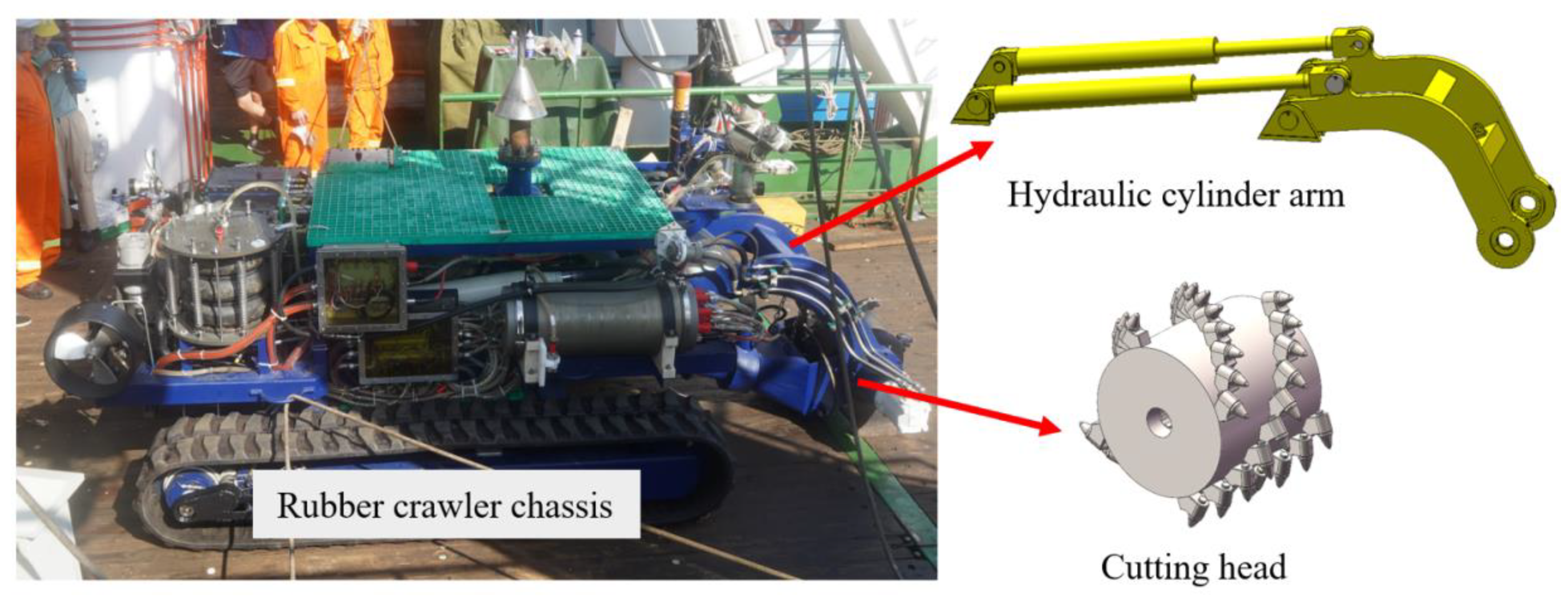
Furthermore, the current mining machines are large and heavy, with high costs, making them unsuitable for preliminary studies. Therefore, the Institute of Deep-Sea Science and Engineering of the Chinese Academy of Sciences (IDSSE, CAS) built a compact seabed CRC mining machine in 2020. The prototype and test results of the mining machine were presented in [9,10]. The design considerations of the mining machine are the crushing and collection of ores and the moving performance of the vehicle.

The main rock breakage mechanisms were considered to be tensile stress failure [11] and shear stress failure [12]. Different pick sizes and shapes [13,14,15], tip and pick materials [13], pick installation parameters, sump depths [16], physical and mechanical properties of the rock [17,18], and installation distances between picks [19] were found to affect the stress of picks and the specific cutting energy of the mining machines. In 2007, Jackson proposed an estimation formula for rock crushing in a high-pressure environment. He concluded that the specific cutting energy of the machine could be estimated according to the rock’s unconfined compressive strength (UCS). This method was used to estimate the cutting resistance and power of the trencher and the mining machine [20]. Roel conducted rock compressive strength and tensile tests under varying hydrostatic pressures in 2013. The tensile strength of the rock was found to increase with increasing depth in the experiment [21]. Miedema proposed a rock-cutting model under hydrostatic pressure in 2015 [22]. In 2020, Balci estimated the specific cutting energy required for rock ore crushing under hydrostatic pressure by comparing the specific cutting energy of a marine in situ drilling rig with that of a land drilling rig. It was estimated that the rock crushing and cutting energy under hydrostatic pressure was 7.7–10.3 times that under land conditions [23]. Therefore, the rock crushing and cutting under hydrostatic pressure is more complex than that on land (hydrostatic pressure, low temperature, microparticle, water drag, etc.), in addition to higher required cutting resistance and power.

The moving performance of the crawler chassis has been studied extensively. In 1969, Bekker put forward the classical theory [24], and Schulte and Wschwarz proposed the empirical relationship between subsidence pressure and depth in deep-sea sedimentation in 2009 [25]. In 2011, Choi conducted a series of tests and fitted the experimental data. The constitutive model of seabed sediments was constructed by the nonlinear shear strength at different depths [26]. In 2016, Wang proposed an elastic soft plastic model suitable for the shear stress displacement model of deep-sea soil, and its effectiveness was verified by a series of seabed simulated soil shear tests [27]. Özdemir proposed a contact model applied to hard ground in 2017, which was in good agreement with reality [28]. Vu studied an up-milling trencher system in 2017 and conducted several simulations using the presented equations for practical design problems and the RC tool analysis [29]. The contact model of the crawler was different under different working conditions. The occurrence area of the CRC was on the seamount, and its terrain should be mainly hard seafloor.

Although some CRC mining vehicles have been designed and tested, the design methods of such mining vehicles are still very limited. Due to the co-existence of crust and substrate, there is a big difference between the mining vehicle and the existing trenching machine in the working process, and the mining vehicle cannot use the design method of the trenching machine. Moreover, the complexity of the CRC environment makes the dynamic relationship between the cutting head and the track of the mining vehicle complex and uncertain. To quickly design the undersea CRC mining machine, reduce the cost of testing and design, and predict the problems in the mining vehicle operation in advance, this paper proposes a modeling method of the CRC mining vehicle based on mining stability. The model is for a slope mining vehicle on seamount and based on the high hydrostatic pressure of rock-specific cutting energy. Mining vehicles’ dimensionless parameters analyze the influence of the stability of mining vehicles under different slope angles, substrate, and crust strength. Finally, the stability of the compact mining vehicle of IDSSE is analyzed and discussed based on two sea trials’ results.

2. Design Requirements

Deposits of the CRC are found throughout the global oceans in the water depth from 450 to 7000 m. The main distribution water depth of the Pacific Ocean is 1000–3500 m [30]. The Western Pacific is more prospective for crust deposits due to more seamounts available. Co- and Ni-rich crust deposits exist, in general, between 800 and 3000 m water depth. These deposits are distributed in flanks, terraces, and summits of seamounts, submerged volcanic mountains, and guyots [31]. Based on more than 11,000 entries, the cumulative mean slope shows two distinct groups of seamount slopes: (1) mountains with slope angles up to about 12°, interpreted as guyots, are about 28% of the total, and (2) mountains with a slope more than 12° (less than 16°), which represent normal conical seamounts, account for about 71% [32].

The crust thickness delineation is 2 cm for the actual thickness from 2.5 to 5.2 cm, and the delineation is 4 cm for the actual thickness from 5.5 to 7.1 cm [30]. The substrate of the crust includes breccia, basalt, phosphorite, limestone, transparent clastic rock, and mudstone. The crusts, in general, are tightly attached to hard substrate rocks. The physical properties of CRC and substrate are in

Table 1. Physical Properties of CRC and substrate.

Physical Properties	CRC	Substrate
UCS	0.5–16.8 MPa	0.1–68.2 MPa
Tensile strength	0.1–2.3 MPa	0.1–18.9 MPa
Porosity (volume %)	52%–66%	18%–47%
Wet bulk density	1.83–20.4 g/cm3	2.04–2.57 g/cm3
Cohesive strength	2.9 MPa	7.8 MPa
Shear strength	1.26–2.5 MPa	-
Angle of internal friction	42°	52°
Young’s modulus	2.15 GPa	0.31–10.1 GPa
P-wave velocity	2.09–4.19 km/s	1.76–5.86 km/s
S-wave velocity	1.35–1.83 km/s	1.15–3.57 km/s

[31,32].

2.1. Mining Process

Since there is no process for CRC mining at present, the mining process of SMS is explained here. The mining process proposed by former Nautilus Minerals for SMS mining is as follows. Firstly, the auxiliary cutter is employed to level the mining surface; then, the ore is crushed by the bulk cutter; finally, the fragmented particles are collected by the hydraulic suction head of the collecting machine and transported to the mining ship by a lifting system. The mining process proposed by JOGMEC is as follows. The swing cutter head in front of the mining vehicle cuts a certain width of the ore, then collects and transfers it to the lifting system by a hydraulic collector. After that, the lifting system transfers the fragmented ore to mining vessels. The sump depth is controlled by the boom of the mining machine [7]. As the crust thickness varies, the sump depth must be controlled during the mining. Typical sump depth control methods include fixed thickness cutting, maximum thickness cutting, and average thickness cutting.

2.1.1. Fixed Depth Cutting

Fixed depth cutting can obtain relatively stable ore output and pick wear rate. The structure and control of the vehicle are relatively simple, as is the machine maintenance. This method suits areas with high concentration and flat stripping surfaces, such as coal mines. However, for the CRC with uneven thickness, microtopography, and substrate, the collection rate, dilution rate, and the wear of picks cannot be controlled.

2.1.2. Maximum Depth Cutting

Maximum depth cutting relies on the CRC thickness detection device. After detecting the thickness of CRC, control the cutting head to adapt to improve the collection rate of CRC and reduce the substrate fragmentation and dilution rate. This method should consider the microtopography adaptation of the cutting head and the detection of CRC thickness. For the microtopography adaption of the cutting head, the hydraulic cylinder controls the sump depth. For the detection of the thickness of the CRC, acoustic detection is used, and the laboratory test is successful [33].

2.1.3. Average Depth Cutting

The average depth cutting is set according to the average thickness of the CRC in the mining area. Given the different physical characteristics between the CRC and substrate, the sump depth can be controlled by the cutting force feedback and adjusted by hydraulic cylinders for microtopography adaption [34]. The hydraulic cylinder applies a constant force in the vertical direction of the cutting head, equal to the force required to cut the CRC of a certain thickness. When the head cuts into the substrate or the microtopography affect the sump depth, the cutting resistance increases, the normal force also increases, and the cutting head can be automatically lifted for adaption, and vice versa. This method cannot avoid cutting the substrate, but the collection and dilution rate of CRC can be controlled by setting the force of the cutting head.

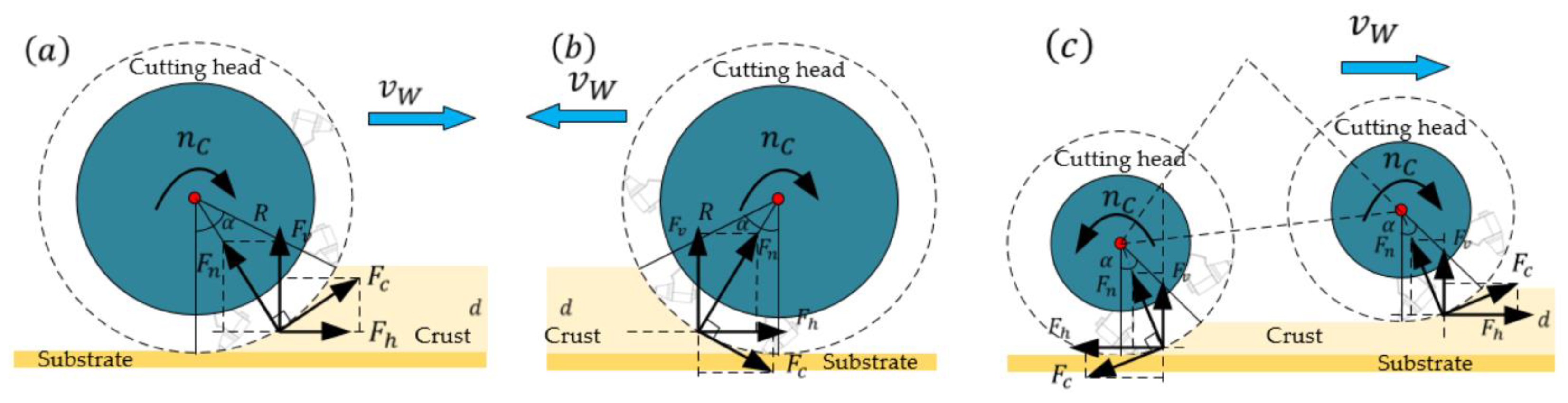
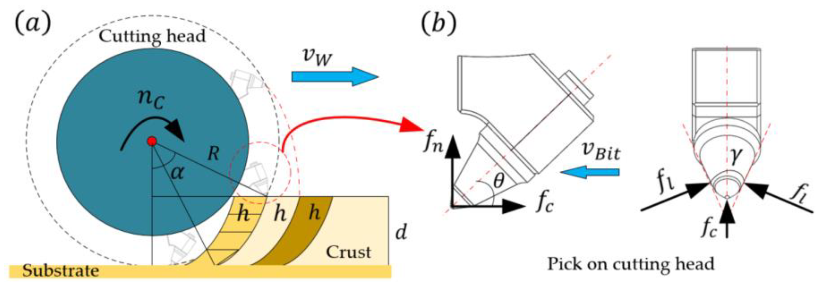
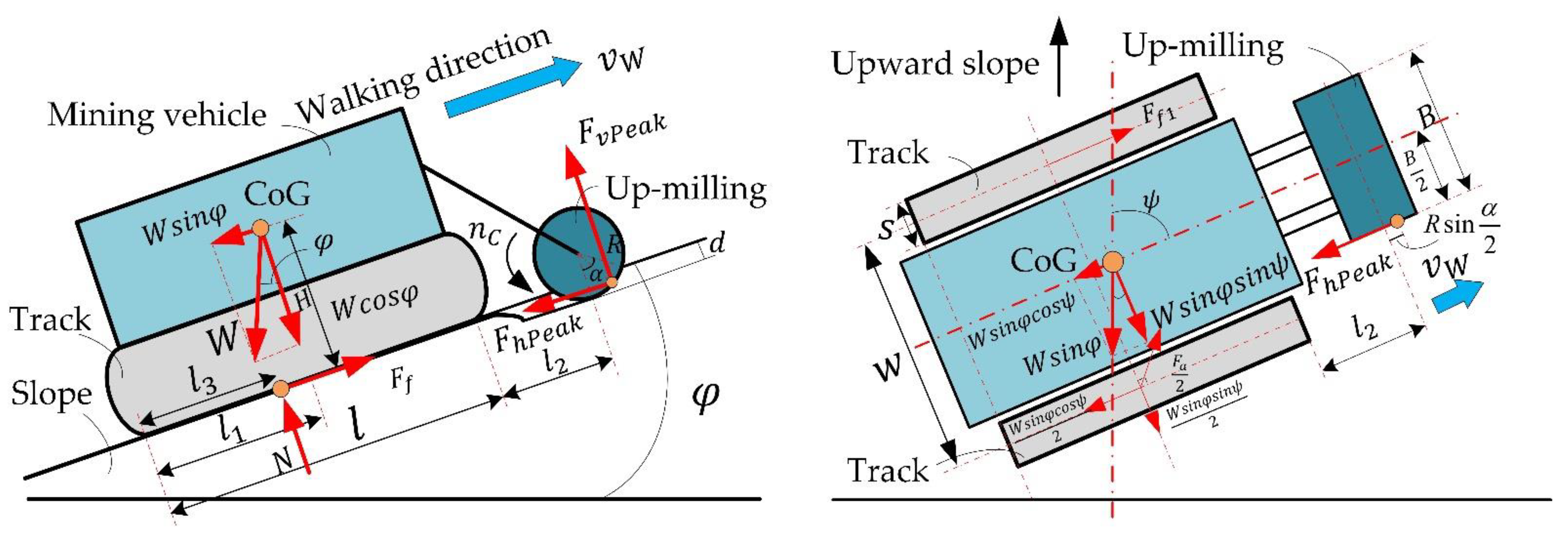
2.2. Cutting Head Structure

Rotary cutting drums are widely used in the cutting head design [34]. The cutting head configuration can be a single drum or dual drums and the structure is shown in Figure 1, The green circle is the cutting head, $n_c$ is the speed of the cutting head, and the arrow is the turning direction, $d$ is the sump depth, $R$ is radius of the cutting head. $v_w$ is the walking speed, and the blue arrow is the direction, $F_c$ is the cutting resistance, $F_n$ is the normal resistance, $F_h$ is the horizontal resistance, $F_v$ is the vertical resistance. $\alpha$ is the contact angle.

2.2.1. Single-Drum

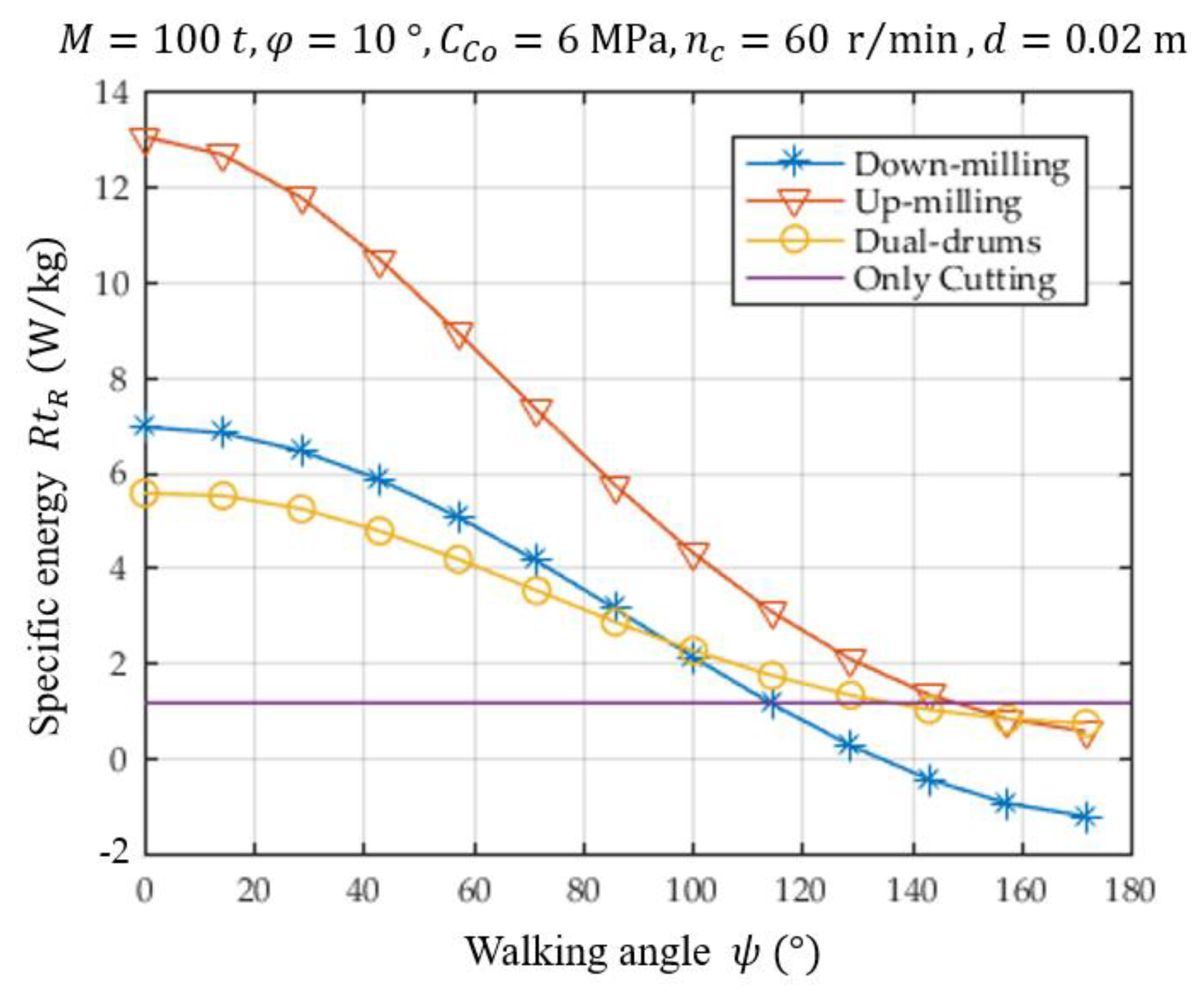
Figure 1a,b is the principle of a single-drum cutting head. The cutting picks of the cutting head are spirally installed outside the drum, and the cutting picks cut the ore through the rotation of the drum. According to the cutting direction, up-milling and down-milling methods are available. In down-milling, the rotation direction of the drum is opposite to the feed direction. Otherwise, it is up-milling. The cutting force of the down-milling produces an extra traction effect, and the cutting force of the up-milling produces an additional resistance.

2.2.2. Dual-Drum

As shown in Figure 1c, the dual-drum cutting head uses two drums arranged symmetrically, and one for up-milling and one for down-milling. The cutting forces of the two cutting heads are opposite and can be partially balanced by each other. The fragmented particles are settled between the two cutting heads and collected by the slurry pump.

3. Analysis on the Force and Moment of the Vehicle

The mining vehicle is mainly subjected to driving resistance, cutting resistance, seawater drag, and umbilical drag in the mining process. The tracked chassis and the tangential component of gravity generate the driving resistance. The cutting resistance is the force generated during the crust crushing, and the direction relies on the cutting method. The seawater drag mainly includes the cutting head rotation’s water drag and the vehicle motion’s resistance.

3.1. Analysis of Cutting Head

3.1.1. Individual Cutter Forces

The specific energy ($E_{sp}$) of the underwater cutting is 100–300% of the rock’s UCS [20]. During the mining vehicle’s design, the UCS of rock can be used to estimate the cutting resistance of trenchers [17], and $S{t}_c$ is the UCS of the ore. Generally, the crushing power of the vehicle is calculated by the average cutting resistance and rotation speed of the cutting head, and the vehicle is designed according to the maximum cutting resistance to ensure vehicle reliability. The average cutting resistance is $F$, which is the sum of cutting resistance generated by each pick of the cutting head and calculated by Equation (2), $N_{\mathit{single}}$ is the number of the picks in each groove, $B$ is the width of the cutting head, and $h$ is the feed per pick (Cutting depth).

$$E_{sp}=S{t}_c,$$

(1)

$$F=S{t}_{c}Bh{N}_{\mathit{single}}.$$

(2)

Figure 2a shows the cutting process. The cutting head traveling speed is $v_w$, the sump depth is $d$, and the cutting head radius is $R$, which determine the contact angle ($\alpha$) of the cutting head and the number of cutting picks engaged. The feed per pick ($h$) is determined by the traveling speed ($v_w$), the rotation speed ($n_c$) of the cutting head, and the number of the picks per groove ($N_{\mathit{single}}$). The contact angle ($\alpha$) is calculated by Equation (3).

$$\alpha =\arccos \left(\frac{R-d}{R}\right).$$

(3)

It is assumed that the diameter of the dual-drum head is half that of the single-drum cutting head, and its sump depth ($d$) is also half that of the single-drum cutting head, and the contact angle is the same as that of the single-drum head. Equation (4) shows the theoretical maximum cutting depth of the cutting head ($\mathsf{\Delta }L$). As the head diameter of the dual-drum cutting head is half that of the single-drum head, the number of picks per groove of the dual-drum cutting head is also half that of the single-drum head. To ensure that the average feed per pick ($h$) is the same, the rotation speed is twice that of the single-drum cutting head. The cutting area per pick is calculated by Equation (5). The average feed per pick (cutting depth) $h$ is calculated by Equation (6). The number of pick lines ($N_{Line}$) is calculated by Equation (7), $R{t}_l$ is the ratio of the pick interval to the average feed per pick, which affects the specific energy of the cutting, and the recommended ratio is 2:5 [19].

$$\mathsf{\Delta }L=\frac{60v_w}{n_c{N}_{\mathit{single}}},$$

(4)

$$S={\displaystyle {\int }_0^{\alpha }R\mathsf{\Delta }L\sin \theta d\theta }=R\left(1-\cos \alpha \right)\mathsf{\Delta }L,$$

(5)

$$h=\frac{1-\cos \alpha }{\alpha }\mathsf{\Delta }L,$$

(6)

$$N_{Line}=\frac{B}{R{t}_{l}h}.$$

(7)

The number of picks of the whole cutting head ($N_{Bit}$) is calculated by Equation (8). As the head diameter of the dual-drum cutting head is half that of the single-drum cutting head, we assume that the number of picks of each line ($N_{\mathit{single}}$) in the dual-drum cutting head is also half that of the single-drum cutting head. Then, the number of picks for simultaneous cutting ($N_{Cut}$) is Equation (9). As the dual-drum head has two drums cutting at the same time, $N_{Cut}$ keeps the same conditions as the single-drum cutting head. The sum of the average cutting resistance of the picks ($F_{cMean}$) within the contact angle is Equation (10). Then, Equation (4) and Equation (6) are substituted into Equation (10), and $F_{cMean}$ can be obtained by Equation (11), The dual-drum head can use also this formula to calculate the resistance.

$$N_{Bit}=N_{Line}{N}_{\mathit{single}},$$

(8)

$$N_{Cut}=\frac{\alpha }{2\pi }{N}_{Bit},$$

(9)

$$F_{cMean}=\frac{\alpha }{2\pi }S{t}_{c}Bh{N}_{\mathit{single}},$$

(10)

$$F_{cMean}=\frac{30\left(1-\cos \alpha \right)S{t}_{c}B{v}_w}{\pi n_c}.$$

(11)

The pick speed is calculated by Equation (12), and substituted into Equation (11), the relationship between the average cutting resistance and the ratio of the pick speed to rotation speed ($R{t}_b$) can be obtained by Equation (13). The average cutting resistance ($F_{cMean}$) on the cutting head is proportional to the sump depth ($d$), cutting head radius ($R$), UCS ($S{t}_c$), and cutting head width ($B$). Forces on a single pick are shown in Figure 2b. The pick is subjected to the horizontal force ($f_c$), normal force ($f_n$), and lateral force ($f_l$) during cutting, so the average cutting resistance on a single pick is calculated by Equation (14). The maximum cutting resistance is about twice that of the average cutting resistance [24], so the maximum cutting resistance is calculated by Equation (15).

$$v_{Bit}=\frac{2\pi R}{60}{n}_{\mathrm{c}},$$

(12)

$$F_{cMean}=\frac{RS{t}_{c}B}{R{t}_b}\left(1-\cos \alpha \right),$$

(13)

$$f_{cMean}=\frac{2\pi RS{t}_{c}B\left(1-\cos \alpha \right)}{\alpha N_{Bit}R{t}_b},$$

(14)

$$f_{cPeak}=2f_{cMean}.$$

(15)

The ratio of the normal cutting force to cutting resistance is $\kappa$, the average and maximum normal cutting force are calculated by Equation (16), When it works on the surface of the microtopography, the forces on individual picks are not even. The pick is subjected to a lateral force on both sides. The average literal force ($f_{lMean}$) and peak literal force ($f_{lPeak}$) can be estimated by Equation (17), where η is the literal force coefficient, $\eta =tan\left(\gamma /2\right)$ [8]. Finally, the three maximum cutting resistances on a single pick can be obtained by Equation (18).

$$\{\begin{array}{l}{f}_{nMean}=\kappa f_{cMean}\\ f_{nPeak}=2\kappa f_{cMean}\end{array},$$

(16)

$$\{\begin{array}{l}{f}_{lMean}=0.5\eta f_{cMean}\\ f_{lPeak}=\eta f_{cMean}\end{array},$$

(17)

$$\{\begin{array}{l}{f}_{cPeak}=\frac{4\pi RS{t}_{c}B\left(1-\cos \alpha \right)}{\alpha N_{Bit}R{t}_b}\\ f_{nPeak}=\frac{4\kappa \pi RS{t}_{c}B\left(1-\cos \alpha \right)}{\alpha N_{Bit}R{t}_b}\\ f_{lPeak}=\frac{2\eta \pi RS{t}_{c}B\left(1-\cos \alpha \right)}{\alpha N_{Bit}R{t}_b}\end{array}.$$

(18)

3.1.2. Forces on Cutting Head

The maximum cutting resistance in the three directions on the cutting head can be obtained by Equation (19). The average and peak cutting resistance torque of the cutting head can be obtained by Equation (20), and the horizontal force ($F_h$) and normal force ($F_v$) on the cutting head, as shown in Figure 1, can be calculated by the cutting forces on picks.

$$\{\begin{array}{l}{F}_{cPeak}={\displaystyle \sum N_{Cut}{f}_{cPeak}=}\frac{60BS{t}_c{v}_w(1-\cos \alpha )}{\pi n_c}\\ F_{nPeak}={\displaystyle \sum N_{Cut}{f}_{nPeak}=}\frac{60\kappa BS{t}_c{v}_w(1-\cos \alpha )}{\pi n_c}\\ F_{lPeak}={\displaystyle \sum N_{Cut}{f}_{lPeak}=}\frac{30\eta BS{t}_c{v}_w(1-\cos \alpha )}{\pi n_c}\end{array}.$$

(19)

$$\{\begin{array}{l}{T}_{Mean}=F_{cMean}R\\ T_{Peak}=2F_{cMean}R\end{array}.$$

(20)

(1)

Forces of down-milling

The cutting resistance is located in the contact angle of the cutting head ($\alpha$). The equivalent cutting resistance is assumed to be in the middle of the contact angle. As shown in Figure 1a, the normal resistance (normal force), horizontal resistance (horizontal force), and lateral resistance (lateral force) of the cutting head can be obtained by Equation (21), $F_v$ is positive in the same direction as the traveling speed. The cutting resistance in three directions can be obtained by substituting the average and maximum cutting resistance into Equation (21).

$$\{\begin{array}{l}{F}_h=F_c\cos \frac{\alpha }{2}-F_n\sin \frac{\alpha }{2}\\ F_v=F_c\sin \frac{\alpha }{2}+F_n\cos \frac{\alpha }{2}\\ F_l=\frac{F_c}{2}\eta \end{array}.$$

(21)

(2)

Forces of up-milling

For up-milling, as shown in Figure 1b, $F_v$, $F_h$, and $F_l$ of the cutting head can be calculated by Equation (22). $F_v$ is in the opposite direction of the traveling speed.

$$\{\begin{array}{l}{F}_h=-F_c\cos \frac{\alpha }{2}-F_n\sin \frac{\alpha }{2}\\ F_v=F_n\cos \frac{\alpha }{2}-F_c\sin \frac{\alpha }{2}\\ F_l=\frac{F_c}{2}\eta \end{array}.$$

(22)

(3)

Forces of dual-drums cutting head

As shown in Figure 1c, the dual-drum cutting head has two cutting resistances in the opposite direction, and the cutting resistances are calculated by Equation (23). By substituting Equation (11) into Equation (23), horizontal cutting resistance, normal cutting resistance, and lateral cutting resistance can be obtained, too.

$$\{\begin{array}{l}{F}_h=-F_n\sin \frac{\alpha }{2}\\ F_v=F_n\cos \frac{\alpha }{2}\\ F_l=F_c\eta \end{array}.$$

(23)

3.1.3. Analysis of Parameter Effects

The parameter values and ranges are listed in

Table 2. Parameters of the cutting head.

Parameters	Notation	Unit	Range	Value
Width of the cutting head	$B$	m	0.2–1	0.5
Radius of the cutting drum	$R$	m	0.1–0.5	0.2
Ratio of lateral force to cutting resistance	$\eta$	—	—	tan(y/2)
Tip angle	$\gamma$	°	—	85
Sump depth	$d$	m	0–0.1	0.04
Ratio of normal force to cutting resistance	$\kappa$	—	—	1.7
Walking speed	$v_w$	m/s	0.01–0.5	0.02
Speed of cutting head	$n_c$	r/min	30–120	60

. The parameter effects in the given range are plotted in Figure 3a–h.

The horizontal forces of three types of cutting heads decrease with the increase in cutting head speed and cutting head radius, as shown in Figure 3a,b. Increasing the cutting head speed can reduce the feed per pick and cutting force. When the radius of the cutting head increases, the contact angle of the cutting head is reduced, and the normal cutting resistance decreases. Figure 3c,d and Equation (19) shows that the horizontal force and vertical force increase with the sump depth, UCS, walking speed, and width of the cutting head, except the sump depth effect of the down-milling horizontal force, as shown in Figure 3c. The horizontal cutting resistance increases and then decreases in the down-milling cutting head as the contact angle changes by the increase in the sump depth, because when the contact angle is small, horizontal force mainly come from lateral force and gradually increases, when the contact angle gradually increases, the radial cutting force increase, which makes the horizontal force increase and then gradually decrease, and reaches the maximum at the sump depth of 0.05 m.

However, the horizontal cutting resistance of the up-milling is 3.6–3.8 times that of the down-milling, and that of the dual-drum head is 1.3–1.4 times that of the down-milling. Thus, the horizontal cutting resistance of the down-milling is the smallest, followed by the dual-drum head. The direction of the horizontal cutting resistance of the up-milling and dual-drum head is opposite to the moving direction of the cutting head, which is the resistance to the walking of the vehicle. The direction of the cutting resistance of the down-milling is the same as the moving direction of the crushing head, which is a help to the walking of the vehicle. The vertical cutting resistance of the up-milling cutting head is 60%–70% of the down-milling cutting head, and that of the dual-drum head is 80%–90% of the down-milling cutting head.

3.2. Walking Resistance

The crawler chassis mainly includes internal friction, external friction, and the tangential gravity component on the slope. Both internal and external friction are resistances, but internal friction does not affect the vehicle’s stability.

3.2.1. External Track Friction

The friction of the mining vehicle on the floor, $F_f$ is calculated by Equation (24). $\mu$ is the friction coefficient between rubber track and rock under wet condition, $\phi$ is the slope angle, $M$ is the mass of the mining machine, and g is the gravity acceleration. The distances from the gravity center to the left and right crawlers are $w_1$ and $w_2$. The average distance is $w=\left(w_1+w_2\right)/2$. The seafloor friction resistances of the left ($F_{fl}$) and right ($F_{fr}$) crawlers are calculated by Equations (25) and (26).

$$F_f=\mu Mg\cos \phi ,$$

(24)

$$F_{fl}=\mu \frac{w_2}{w}Mg\cos \phi ,$$

(25)

$$F_{fr}=\mu \frac{w_1}{w}Mg\cos \phi .$$

(26)

3.2.2. Tangential Component of Gravity

When the mining vehicle walks on the slope, the tangential component of the gravity ($F_s$) is calculated by Equation (27), W is the submerged weight of the vehicle, $\phi$ is the slope angle, and $\psi$ is the direction angle when walking up the slope, $\psi =0$, when walking down the slope, $\psi =180˚$.

$$F_s=W\sin \phi \cos \psi .$$

(27)

3.3. Friction and Friction Torque for Stabilities

The friction on both tracks should be big enough to avoid slipping and skidding in the operation on the slope. The mining vehicle walks on the seamount with the hard floor, which is rock. Therefore, Coulomb friction applies.

3.3.1. Anti-Slip Friction

When the cutting force exceeds the track friction, the vehicle slips on the slope. The friction of the mining vehicle ($F_a$) is calculated by Equation (28), $\lambda$ is the friction coefficient, $\phi$ is the slope angle, and $F_{vPeak}$ is the maximum normal cutting resistance.

$$F_a=\lambda \left(W\cos \phi -F_{vPeak}\right).$$

(28)

3.3.2. Anti-Skid Friction Torque

When the external torque applied to the vehicle exceeds the track friction torque, the vehicle rotates around a point of O on the track, and the skid happens. The friction torque ($T_f$) can be obtained by the torque integral on the track area about the rotation point. The friction per unit area of the track chassis ($\mathsf{\Delta }f$) is calculated by Equation (29), $s$ is the track width and $l$ is the track contact length. As shown in Figure 4, the two gray rectangles represent two tracks, and the green rectangle represents the cutting head, the vehicle rotates about orange point O, and the orange point W is the center of the vehicle so the friction torque can be obtained by Equation (30).

$$\mathsf{\Delta }f=\frac{F_a}{2sl},$$

(29)

$$T_f=\mathsf{\Delta }f\left({\displaystyle {\int }_{x_1}^{x_2}{\displaystyle {\int }_{y_2}^{y_1}\sqrt{x^2+y^2}dxdy}}+{\displaystyle {\int }_{x_1}^{x_2}{\displaystyle {\int }_{y_4}^{y_3}\sqrt{x^2+y^2}dxdy}}\right).$$

(30)

3.4. Analytical Model on the Power and Systemic Performance Index

3.4.1. Power Consumption for Mining

The power consumption for mining includes power for walking and cutting. The power consumption is calculated by Equation (31). The walking resistance on the slope includes the track friction, the tangential gravity component, and cutting force, and can be calculated by Equation (32). The walking power can be calculated by Equation (33). The cutting power can be calculated by Equation (34).

$$P=P_{Walking}+P_{Cutting},$$

(31)

$$f_{Walking}=\mu \left(W\cos \phi -F_v\right)+W\sin \phi \cos \psi -F_h,$$

(32)

$$P_{Walking}=\left(\mu \left(W\cos \phi -F_v\right)+W\sin \phi \cos \psi -F_h\right)v_w,$$

(33)

$$P_{Cutting}=F_{cMean}{v}_{Bit}.$$

(34)

When the mining vehicle moves down the slope ($\psi >90°$), the walking resistance $f_{Walking}$ decreases as an effect of the tangential gravity component. When $f_{Walking}=0$, we can get Equation (35). The traveling angle of the mining vehicle (${\psi }_1$) is calculated by Equation (36). Finally, the total power consumption is calculated by Equation (37). Substituting Equations (21) and (23) into Equation (37), the mining power of the up-milling, down-milling, and dual-drum heads can be calculated, too.

$$\mu \left(W\cos \phi -F_v\right)+W\sin \phi \cos \psi -F_h=0,$$

(35)

$${\psi }_1=\arccos \left(\frac{F_h-\mu \left(W\cos \phi -F_v\right)}{W\sin \phi }\right),$$

(36)

$$\{\begin{array}{ll}P=\left(\mu \left(W\cos \phi -F_v\right)+W\sin \phi \cos \psi -F_h\right)v_w+F_{cMean}{v}_{Bit}& \left(0\le \psi \le {\psi }_1\right)\\ P=F_{cMean}{v}_{Bit}& \left({\psi }_1<\psi \right)\end{array},$$

(37)

3.4.2. Specific Yield Mass

Generally, when the crushing rate (area ratio of broken crust per unit area) is 80%, the wet density of CRC is 1.8 t/m³ [5], working for 200 days per year and 18 h per day. The mining yield of the vehicle is the mass of the ore crushed per hour. Then, the yield of the mining vehicle ($Y$) is calculated by Equation (38), $B$ is the cutting head width, $d$ is the sump depth, and $v_w$ is the walking speed of the mining vehicle. To evaluate the mining vehicle’s performance, we define the specific yield ($R{t}_p$) as the yield ratio to the mining vehicle mass and calculate by Equation (39), $M$ is the mass of the mining vehicle. For the design of the mining vehicle, the higher the specific yield is, the better. In the same way, the specific cutting force to the vehicle mass is calculated by Equation (40). The specific cutting forces in three directions are shown in Equation (41).

$$Y=5184000Bd{v}_{\mathrm{w}}\left(\mathrm{kg}/\mathrm{h}\right),$$

(38)

$$R{t}_p=\frac{Y}{M}=\frac{5184000Bd{v}_w}{M},$$

(39)

$$\frac{F_{cMean}}{M}=\frac{\left(1-\cos \alpha \right)S{t}_{c}R{t}_p}{172800d\pi n_c},$$

(40)

$$\{\begin{array}{l}\frac{F_{cPeak}}{M}=\frac{S{t}_c(1-\cos \alpha )R{t}_p}{86400d\pi n_c}\\ \frac{F_{nPeak}}{M}=\frac{\kappa S{t}_c(1-\cos \alpha )R{t}_p}{86400d\pi n_c}\\ \frac{F_{lPeak}}{M}=\frac{\eta S{t}_c(1-\cos \alpha )R{t}_p}{172800d\pi n_c}\end{array}.$$

(41)

3.4.3. Specific Mining Power

The specific mining power to the vehicle mass ($R{t}_{Power}$) is employed to evaluate the power consumption of the different mining vehicles, and it is calculated by Equation (42).

$$\{\begin{array}{ll}R{t}_{Power}=\left(\mu \left(g\cos \phi -\frac{F_v}{M}\right)+g\sin \phi \cos \psi -\frac{F_h}{M}\right)v_w+\frac{F_{cMean}}{M}{v}_{Bit}& \left(0\le \psi \le {\psi }_1\right)\\ R{t}_{Power}=\frac{F_{cMean}}{M}{v}_{Bit}& \left({\psi }_1<\psi \right) \end{array}.$$

(42)

3.4.4. Specific Mining Energy

The specific energy ($R{t}_R$) is employed to evaluate the power consumption for unit mass of the ore, defined as the ratio of the total power to the yield, and calculated by Equation (43). Therefore, substituting the total power and yield into Equation (43), the specific energy of the three different mining vehicles can be compared in energy cost.

$$R{t}_R=\frac{P}{Y}=\frac{P}{M}\times \frac{M}{Y}=\frac{R{t}_{Power}}{R{t}_p}\left(\mathrm{W}/\mathrm{Kg}\right).$$

(43)

4. Working Stability Analysis of Mining Vehicles

The following assumptions are made for the stability analysis:

• The gravity center of the mining vehicle is at the center of the chassis, and the loads on the two tracks are the same.
• The width of the cutting head does not exceed the width of the chassis.
• When the mining vehicle cuts the substrate by a depth of d, the cutting head is lifted up to reduce the cutting force but still cuts the substrate by a depth of $\epsilon d$. Therefore, the contact angle ($\alpha$) reduces to ($\beta$):

  $$\beta =\arccos \left(1-\epsilon R{t}_b\right)$$

  (44)

• The cutting head adjusting system can also be used to reduce the dynamic load’s impact on the mining vehicle’s driving performance.

4.1. Working Stability

The working stability includes slope, anti-slip (translational motion), and anti-skid (rotational motion) stability.

4.1.1. Slope Working Stability Condition

When mining on a slope, the vertical cutting force tends to jack up the vehicle in the front, and the tracks and vehicle cannot walk properly, as shown in Figure 5. When the vehicle works on a slope, the cutting head is subjected to $F_{vPeak}$ and $F_{hPeak}$, gravity ($W$), and slope support ($N$). The torque generated by the cutting force on the mining vehicle should not exceed the torque generated by gravity, as shown in Equation (45). $l_1$ is the distance between the gravity center and the rear end of the track, $l_2$ is the distance between the cutting head and the front end of the track, $l_3$ is the distance from the equivalent support point of the track to the rear end of the track, and $l$ is the length of the track contact surface.

$$F_{vPeak}\cdot \left(l_2+l+R\sin \frac{\alpha }{2}\right)+W\sin \phi \cos \psi \cdot H+F_{hPeak}\left(d-R\left(1-\cos \frac{\alpha }{2}\right)\right)\le W\cos \phi \cdot l_1,$$

(45)

4.1.2. Anti-Slip Stability Condition

Both tracks cannot slip on the slope when the vehicle is subjected to the maximum cutting force, as shown in Figure 6. If the vector sum of the horizontal force ($F_{hPeak}$) and the tangential gravity component exceeds the track friction, a slip happens. The following relation of Equation (46) needs to be met to ensure no slip happens.

$${\left(F_{hPeak}\left(\frac{w+B}{2w}\right)+\frac{W\sin \phi \cos \psi }{2}\right)}^2+{\left(\frac{W\sin \phi \sin \psi }{2}\right)}^2\le {\left(\frac{F_a}{2}\right)}^2.$$

(46)

4.1.3. Anti-Skid Steering Stability Condition

Anti-skid stability ensures no slip in the rotation when the mining vehicle works with the maximum cutting force. Figure 7 shows how the vehicle works with the maximum cutting force on the slope, with the dual-drum head as an example. The cutting head is subjected to horizontal cutting resistance $F_{hPeak}$, normal cutting resistance $F_{vPeak}$, lateral cutting resistance $F_{lPeak}$, gravity, and track friction. The cutting forces generate torque in the surface plane of the slope about a point of O on the lift track. The Equation (47) needs to be met to ensure no skid happens, $F_{vPeak}$ is the maximum normal cutting resistance, $F_{hPeak}$ is the maximum horizontal cutting resistance generated by the cut on the substrate by the depth of $\epsilon d,$ the compressive strength ($S{t}_c$) is the UCS of the substrate($C_{Rock}$), and the cutting contact angle is $\beta$.

$$\begin{array}{l}{F}_{lPeak}\left(\frac{\left(l+l_2+R\sin \frac{\beta }{2}-l_1\right)W\cos \phi }{W\cos \phi -F_{vPeak}}\right)+F_{hPeak}\left(\frac{w}{2}+\frac{B}{2}\right)\\ +W\sin \phi \sin \psi \left(\frac{F_{vPeak}\left(l_2-l_1+l+R\sin \frac{\beta }{2}\right)}{W\cos \phi -F_{vPeak}}\right)+W\sin \phi \cos \psi \left(\frac{w}{2}\right)\le T_f , \end{array}$$

(47)

4.2. Stability Analysis

The vehicle’s structural dimensions were normalized and are listed in

Table 3. Ratios and their value ranges.

Notation	Describe	Range	Value
$R{t}_d=d/R$	Ratio of sump depth to cutting head radius	$0.1 –0.5$	0.1
$R{t}_1=l_1/l$	Ratio of center of gravity position to track grounding length	$0.5 –0.9$	0.5
$R{t}_2=l_2/l$	Ratio of cutting head position to track grounding length	$-0.5 –0.5$	0.25
$R{t}_H=H/l$	Ratio of gravity height of the vehicle to track grounding length	$0 –+\infty$	0.25
$R{t}_w=w/l$	Ratio of track gauge to track grounding length	$0.5 –1.2$	0.5
$R{t}_B=B/l$	Ratio of cutting head width to track grounding length	$0 –+\infty$	0.2
$R{t}_s=s/l$	Ratio of track shoes width to track grounding length	$0 –+\infty$	0.2
$R{t}_c=R/l$	Ratio of cutting head radius to track grounding length	$0.1 –0.5$	0.2

. The structural parameters are transformed into ratios with regard to the length of the crawler and the radius of the crushing head. The parameters for the stability analysis are listed in

Table 4. Parameters for the stability analysis.

Parameters	Notation	Unit	Range	Value
Static friction coefficient	$\lambda$	—	—	0.9
Slope angle	$\phi$	°	—	10
Walking angle	$\psi$	°	0–180	—
UCS of the CRC	$C_{Co}$	MPa	—	6
UCS of the substrate	$C_{Ro}$	MPa	—	68.2
Ratio of sump depth for substrate cutting	$\epsilon$	—	0–1	0.5
Mass of the mining vehicle	$M$	$\mathrm{kg}$	—	100,000
Width of the cutting head	$B$	$\mathrm{m}$	—	4
Sump depth	$d$	$\mathrm{m}$	—	0.02

.

4.2.1. Stability Analysis of Three Types of Mining Vehicles

Based on the working stability of three types of mining vehicles in Equations (45)–(47), the specific yields of the mining vehicle ($R{t}_p$) about the direction angles on the slope are plotted in Figure 8, and the stability conditions are solved by Newton’s iterative method. The walking direction affects the stability of the mining vehicle on the same slope, and the impact is related to the structure of the mining vehicle. As shown in Figure 8a, the stability of the mining vehicle with the dual-drum head is the best and produces the maximum specific yield. Figure 8b shows the specific yields of the three types of vehicles with the anti-slip condition. The dual-drum type has the highest stability, followed by the up-milling type. The main reason is that the symmetrical drum structure makes the cutting resistances partially balanced and minimizes the impact of the cutting resistance. The average stability of the up-milling type is slightly higher than that of the down-milling type, mainly because the normal cutting resistance of the up-milling type is slightly lower than that of the down-milling type. As shown in Figure 8c, the stability of the mining vehicle with the dual-drum type is better than that of the up-milling and down-milling types.

Walking straight up and down is not recommended for these three mining vehicles when considering the slip and skid stability. Instead, spirally walking up and down is better to minimize stability risk. The down-milling type is better for adopting the mining strategy of spirally walking from the bottom to the top of the mountain. On the contrary, the up-milling and dual-drum types are better for walking from the top to the bottom of the slope. The specific yield of the single-drum type is lower than that of the dual-drum type, which indicates that the weight of the dual-drum type is lighter with the same yield. However, the dual-drum type structure is more complex than the single-drum type.

4.2.2. Analysis of Structural Parameters on Stability

The influence of the cutting head position on stability is shown in Figure 9. The ratio $R{t}_2$ affects slope stability and anti-slip stability. In these two stability conditions, the specific yield of the three types of mining vehicles decreases with the increase in $R{t}_2$, which also shows that the shorter the distance from the cutting head to the middle of the mining vehicle is, the better.

Figure 10 shows the influence of the position of the gravity center on slope stability and anti-skid stability. The center of gravity should be close to the front of the mining vehicle to improve the on-slope stability. For anti-skid stability, if the gravity center is close to the front or the back, the stability is better than in the middle of the vehicle. When the skid center is located in the front or back of the mining vehicle, the anti-skid friction torque is improved. Figure 11 shows the influence of the sump depth on the stability. It is negatively correlated with three stabilities. When the value of $R{t}_d$ increases, the contact angle increases and results in an increased normal cutting resistance and low specific yield and stability. The slope stabilities are positively correlated with the track width, except for the up-milling type, as shown in Figure 12a. As shown in Figure 12b, the anti-skid stability of the mining vehicle is positively correlated with the track width ratio of the mining vehicle ($R{t}_w$) for all three types of mining vehicles.

4.2.3. Specific Energy of the Mining Vehicle

The mining vehicle’s specific yield ($R{t}_p$) is calculated based on the sump depth and the cutting head speed with the stability conditions. Then, we substitute the three mining vehicles’ walking speeds into Equation (42) to calculate the specific energy ($R{t}_R$). Finally, the specific energies of the three mining vehicles can be obtained by Equation (43). Figure 13 shows the specific energy of the three mining vehicles and cutting types. The walking direction changes from uphill to downhill as the driving angle increases and the specific energy ($R{t}_R$) gradually decreases until the driving resistance of the mining vehicle is fully balanced by gravity, as shown in Figure 13. The energy consumption for cutting is a horizontal straight line in Figure 13, with a specific energy of 1.1574 W/kg. The specific energy of the up-milling is 11.2 times that of the cutting-only specific energy. The specific mining energy decreases to the specific energy of the cutting-only, 1.1574 W/kg, when the walking angle is 148°. The specific energy of the down-milling is 6.9 times that of the specific energy of the cutting only. It decreases to the cutting-only specific energy at a walking angle of 113°. The specific energy of the dual-drum type is 4.8 times that of the cutting only and decreases to the cutting-only specific energy at a walking angle of 136°.

The specific mining energy of the dual-drum type is the lowest, followed by the down-milling type. However, the structure of the dual-drum type is more complex and costs more for maintenance compared with the single-drum cutting head. Moreover, particles settle between the two drums. If they are not collected in time, this will cause excessive cutting and waste more energy. Walking spirally up or down a hill can stabilize the energy consumption of the mining vehicle during the mining process and avoid walking directly uphill and downhill. The specific mining energy of the up-milling vehicle is more sensitive to the walking angle than the down-milling vehicle.

5. Case Study and Discussion

5.1. Structure and Parameters of Mining Vehicle

The down-milling mining vehicle is fabricated with a hydraulic cylinder to control the cutting head up and down, as shown in Figure 14. The jet pump is behind the cutting head for the collection of crushed ore. The structural parameters of the vehicle are listed in

Table 5. Parameters of mining vehicle.

Parameters	Notation	Unit	Value
Cutting head width	$B$	$\mathrm{m}$	0.4
Radius of cutting head	$R$	$\mathrm{m}$	0.2
Tip angle of pick	$\gamma$	$°$	80
Cutting depth	$h$	$\mathrm{m}$	0.02
Ratio of space to depth	$R_t$	-	2
Pick distribution coefficient	$C_{bit}$	-	1
Sump depth	$d$	$\mathrm{m}$	0.02
Traveling speed	$v$	$\mathrm{m}$	0.02
Speed of cutting head	$n_c$	$\mathrm{rev}/\min$	60
Cutting angle	$\xi$	$°$	60
Number of picks per lines	$N_{single}$	-	2
Underwater mass of vehicle	$M$	$\mathrm{kg}$.	3200
Distance of center of gravity	$l_1$	$\mathrm{m}$	1.36
Distance of cutting head to the	$l_2$	$\mathrm{m}$	3.057
Adhesion coefficient of track chassis	$\lambda$	-	0.9
Water drag coefficient	$K_w$	-	0.9
Seawater density	$\rho$	$\mathrm{kg}/{\mathrm{m}}^3$	1025
Track grounding length	$l$	$\mathrm{m}$	2.057
Track width	$s$	$\mathrm{m}$	0.35
Track gauge	$w$	$\mathrm{m}$	1.65
Track-rolling friction coefficient	$\mu$	-	0.1
Water-facing area	$A_1$	${\mathrm{m}}^2$	1.5
Center of gravity height	$H$	$\mathrm{m}$	0.65

. The force of the cutting head on the seafloor can be calculated by Equation (48) as, where the constant term is the weight of the booms and the cutting head, $P_{Cylinder}$ is the pressure in the cylinder.

$$F=2126.2\times P_{Cylinder}+6227.1,$$

(48)

5.2. Analysis of Crushing Process Parameters

The umbilical remotely controls the mining vehicle during the test, and the support vessel needs to follow at a certain speed during the mining process of the vehicle. According to the design of the mining vehicle, the maximum walking speed is 0.05 $\mathrm{m}/\mathrm{s}$. The mining vehicle walks and cuts the uneven surface, and the sump depth and UCS of the rocks are not constant. We set the rotation speed of the cutting head and the force on the cutting head to make it contact the seafloor for mining. The yield, walking speed range, sump depth, and normal force range can be calculated under the anti-skid stability condition, and they decrease with the slope increase, as shown in Figure 15.

5.3. Sea Trials

We have conducted two sea trials about the systems function tests in the South China Sea. Due to the costs, the system does not add additional force sensors to measure the cutting force and the force that make the cutter head contact with the seafloor. However, we set the max cutting head pressure, measured the hydraulic cylinder pressure instead, and calculated the force to make the cutter head contact with the seafloor by Equation (48). The depth sensor ISD4000 (From the company of ImpactSubsea) is employed to measure the heading Pitch and roll of the vehicle. The parameters are shown in

Table 6. Parameters of ISD4000.

Parameter	Range	Accuracy	Resolution
Depth	600Bar	±0.01% Full Scale	0.001% Full Scale
Pitch	±90°	0.2°	0.1°
Roll	±180°	0.2°	0.1°
Heading	360°	±0.5°	0.1°

. We measure the hydraulic cylinder pressure with a pressure gauge, and the gauge’s parameters are shown in

Table 7. The parameters of pressure gauge for hydraulic cylinder.

Type	Manufacturer	Accuracy Class	Range
YN-60	Tian Jin MRT	1.6	0~10 MPa

.

The sea trials were as follows:

(1)

First sea trial of the mining vehicle in the South China Sea

The first sea trial took place in April 2019, the site of the first sea trial was the seamount of the South China Sea, and the support vessel was “Hai Yang Liu Hao” of the Guangzhou Geological Survey. The longitude and latitude of the sea trial were 115°06.1626′ E and 18°17.7289′ N, and the water depth was 2493 $\mathrm{m}$. According to other studies, basalt is the main rock in the area of the South China Sea [35]. The heading, pitch, and roll changed during the walking and cutting, which is shown in Figure 16a. The vehicle is walking up to the seamount on a 29° slope. The vehicle only walks, and the roll and pitch change about 1° before 60 s. After 60 s, the vehicle cuts during walking. The pitch changes to 29° to 32°. The heading changes by about 2.2° during 50 s. There are about 2 kg of particles collected from this test, shown in Figure 16b. During the sea trial, the traveling speed was set to about 0.05 m/s, and the pressure of the hydraulic cylinder was 0.65 MPa. As shown in Figure 17, the preload was 7609 N by considering the weight of the cutting head, according to Equation (48). When the head cuts the substrate, the reaction force is 11,011 N.

(2)

The second sea trial of the mining vehicle in the South China Sea

The support vessel of the mining vehicle in the second sea trial was “Tan Suo Er Hao”. The longitude and latitude of the sea trial were 114.85256 E and 13.399554 N, and the water depth was 1329 m. Before diving, an environmental survey was conducted in the test area with the manned submersible “Shen Hai Yong Shi”, and the hard flat area was selected for the sea trial. During the mining test, the traveling speed of the mining vehicle was 0.05 m/s. The rock strength was relatively low and covered with sediment. The heading, pitch, and roll are shown in Figure 18a. The working place is flat and the slope angle is 0–2°, the heading changes no more than 1°. There are about 6.6 kg of particles collected from this test, shown in Figure 18b. According to the video of the hydraulic gauge from 22:21:16 to 22:21:20 (about 4 s) in Figure 19, the hydraulic cylinder pressure varied from 1 to 1.6 MPa. The reaction force of the cutting head was calculated as 8353–10,479 N.

(1)

Result discussion

Although two mining tests of mining vehicles with different depths and working parameters have been successful, rock particles have been broken and collected. We can still find that the stability of the first mining vehicle is far lower than that of the second sea trial. The parameters of the two sea trials show in

Table 8. The parameters of the two sea trials.

Date	Depth	Slope Angle	Walking Speed	Hydraulic Pressure	Stable
2019.4	2493 m	29°	0.05 m/s	0.65–2.25 MPa	No
2020.9	1329 m	0~2°	0.05 m/s	1–1.6 MPa	Yes

. Figure 15 shows the vehicle has shallow sump depth when it walks at 0.05 m/s and 29° slope angle. There is much evidence that has shown the first mining test is unstable. Firstly, the pitch and heading in Figure 16 were stable before cutting, but when the mining test began, the pitch got bigger, and the heading got bigger, too. It indicates the vehicle was not straight walking, and the skid steer had taken place. The pitch and heading in Figure 18 change a little. The video also shows the skid from 18:42:42 to 18:42:46 (about 4 s) during the test. The reference object in the video, coral, has shifted to the right, shown in Figure 20. It is also shown the first mining test’s grooves of the mining is not straight and turn to the port side, and the second mining test’s grooves are straight in Figure 21a.

Many parameters can affect the vehicle’s stability during sea trials. First, the slope angle decreases the vehicle’s vertical contact force on the slope and decreases the vehicle’s resistance and anti-skid friction torque, and decreases the stability at last. Second, the substrate and crusts of the first mining place have more high strength than the second place. We can find out by the cylinder’s pressure during cutting. The first test achieved more significant normal resistance which will also decrease the vehicle’s vertical contact force on the slope. The rough surface will affect the vehicle’s pitch and roll while walking, but the influence will decrease when the vehicle begins to cut, as shown in Figure 16. The roll change is due to the rough seafloor before 60 s, and the vehicle cuts during walking after 60 s. The roll is mostly stable, and there are some changes due to the rough surface. Therefore, the strength of the substrate, crusts, and slope angle significantly impact the mining vehicle’s stability and need to be fully investigated before business mining. The mining site’s microtopography may affect the vehicle’s pitch and roll and needs to be investigated, too.

6. Conclusions

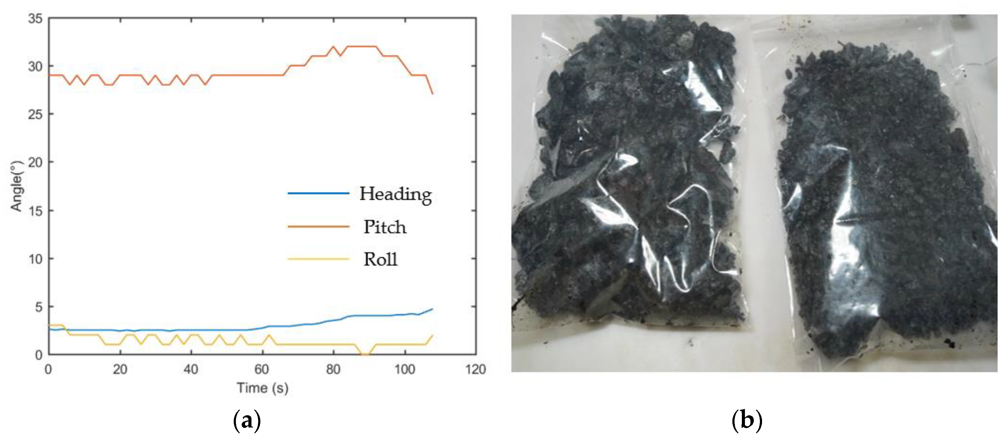
The authors proposed a modeling method for estimating the performance of the mining vehicle based on the mining vehicle’ slope stability, anti-slip stability, and anti-skid steering stability condition. The model adopted the dimensionless parameters of the mining vehicle’s structure. The influence of the mining vehicles under different slope angles, substrate, and crust strength is obtained. Then, three types of mining vehicles’ specific energy are provided based on anti-slip stability conditions. The double drum mining vehicle has the lowest specific energy, followed by the down-milling type, and the last one is the up-milling type by comparison. Finally, the performance of a compact mining vehicle’s mining stability is provided. Two sea trials’ test results are given; from the mining tests, the slope angle, substrate’s, and crust’s strength significantly influence the vehicle’s mining stability. The modeling method in this paper considers the influence of the slope angle, dimensionless parameters, substrate, and crust strength, which will provide a better estimation during the mining vehicle’s design. However, the influence of factors such as pick distribution, pick installation angle, pick material, and current in the working area has been ignored to simplify the modeling process. A more accurate model will be one of our future works.

References

1. Miller, K.A.; Thompson, K.F.; Johnston, P.; Santillo, D. An Overview of Seabed Mining Including the Current State of Development, Environmental Impacts, and Knowledge Gaps. Front. Mar. Sci. 2018, 4, 418. [Google Scholar] [CrossRef] [Green Version]
2. Hein, J.R.; Mizell, K.; Koschinsky, A.; Conrad, T.A. Deep-ocean mineral deposits as a source of critical metals for high- and green-technology applications: Comparison with land-based resources. Ore Geol. Rev. 2013, 51, 1–14. [Google Scholar] [CrossRef]
3. JPI OCEANS Mining Impact. Available online: https://www.jpi-oceans.eu/en/miningimpact (accessed on 25 October 2022).
4. Managine Impacts of Deep Sea Resource Exploitation. Available online: https://www.eu-midas.net/ (accessed on 25 October 2022).
5. Halkyard, J. Technology for mining cobalt rich manganese crusts from seamounts. In Proceedings of the OCEANS ‘85—Ocean Engineering and the Environment, San Diego, CA, USA, 12–14 November 1985. [Google Scholar]
6. Nautilus Minerals Unveils its Titanic Deep Sea Mining Machines. Available online: https://www.mining-technology.com/analysis/featurenautilus-minerals-unveils-its-titanic-deep-sea-mining-machines-4739435/ (accessed on 7 January 2022).
7. Yamaji, N.; Okamoto, N.; Shiokawa, S.; Kawano, S.; Sakurai, H. Achievement for Pilot Test of Excavating and Ore Lifting Conducted for Seafloor Polymetallic Sulphides. J. MMIJ 2019, 135, 42–51. [Google Scholar] [CrossRef] [Green Version]
8. JOGMEC Conducts World’s First Successful Excavation of Cobalt-Rich Seabed in the Deep Ocean; Excavation Test Seeks to Identify Best Practices to Access Essential Green Technology Ingredients while Minimizing Environmental Impact. Available online: https://www.jogmec.go.jp/english/news/release/news_01_000033.html (accessed on 25 October 2022).
9. Yang, N.; Xie, C.; Chen, Y.; Chen, M.; Zheng, J.; Zhang, M.; Li, L. The Design of Sampling Machine for Mineral Resources. In Proceedings of the Twenty-Seventh (2017) International Ocean and Polar Engineering Conference, San Francisco, CA, USA, 25–30 June 2017. [Google Scholar]
10. Xie, C.; Wang, L.; Yang, N.; Agee, C.; Chen, M.; Zheng, J.; Liu, J.; Chen, Y.; Xu, L.; Qu, Z.; et al. A Compact Design of Underwater Mining Vehicle for the Cobalt-Rich Crust with General Support Vessel Part A: Prototype and Tests. J. Mar. Sci. Engineering. 2022, 10, 135. [Google Scholar] [CrossRef]
11. Evans, I. The force required to cut coal with blunt wedges. Int. J. Rock Mech. Min. Sci. Geomech. Abstr. 1965, 2, 1–12. [Google Scholar] [CrossRef]
12. Nishimatsu, Y. The mechanics of the rock cutting. Int. J. Rock Mech. Min. Sci. Geomech. Abstr. 1972, 9, 261–270. [Google Scholar] [CrossRef]
13. Miller, M.H.; Sikarskie, D.L. On the penetration of rock by three-dimensional indentors. Int. J. Rock Mech. Min. Sci. Geomech. Abstr. 1968, 5, 375–398. [Google Scholar] [CrossRef] [Green Version]
14. Roxborough, F.F.; King, P.; Pedroncelli, E.J. Tests on the cutting performance of a continuous miner. J. South Afr. Inst. Min. Metall. 1981, 81, 9–25. [Google Scholar]
15. Qayyum, R.A. Effects of Bit Geometry in Multiple Bit-Rock Interaction. Master’s Thesis, West Virginia University, Morgantown, WV, USA, 2003; pp. 36–61. [Google Scholar]
16. Hurt, K.G.; MacAndrew, K.M. Cutting Efficiency and life of rock-cutting picks. Min. Sci. Technol. 1985, 2, 139–151. [Google Scholar] [CrossRef]
17. Evans, I. A theory of the cutting resistance for point-attack picks. Int. J. Min. Eng. 1984, 2, 63–71. [Google Scholar] [CrossRef]
18. Goktan, R.M. A suggested improvement on Evans cutting theory for conical bits. In Proceedings of the Fourth International Symposium on Mine Mechanization and Automation, Brisbane, QLD, Australia, 6–9 July 1997; Gurgenci, H., Hood, M., Eds.; Cooperative Research Centre for Mining Technology and Equipment: Kenmore, QLD, Australia, 1997; Volume 1, pp. 57–61. [Google Scholar]
19. Khair, A.W. Research and Innovations for Continuous Miner’s Cutting Head for Efficient Cutting process of rock/coal. In Proceedings of the 17th International Mining Congress and Exhibition of Turkey, Ankara, Turkey, 19–22 June 2001. [Google Scholar]
20. Jackson, E.; Devaux, M.D.; Machin, J. Performance Prediction for a Subsea Mechanical Trenching Wheel. In Proceedings of the 6th International Offshore Site Investigation and Geotechnics Conference, London, UK, 11–13 September 2007. [Google Scholar]
21. Kuiper, R.J.; Miedema, S.A.; Frumau, J.; Rhee, C. Influence of the Hyperbaric Effect on Apparent Material Strength of Fully Saturated Porous Rock for Low Strain Rates. In Proceedings of the Offshore Technology Conference, Houston, TX, USA, 6–9 May 2013. [Google Scholar]
22. Miedema, S.A. The Delft Sand, Clay & Rock Cutting Model., 3rd ed.; Tu Delft open: Delft, Netherlands, 2019; pp. 297–324. [Google Scholar]
23. Balci, C.; Copur, H.; Bilgin, N.; Ozdemir, L.; Jones, G.R. Cuttability and drillability studies towards predicting performance of mechanical miners excavating in hyperbaric conditions of deep seafloor mining. Int. J. Rock Mech. Min. Sci. 2020, 130, 104338. [Google Scholar] [CrossRef]
24. Bekker, M.G. Introduction to Terrain-Vehicle Systems; The University of Michigan Press: Ann Arbor, MI, USA, 1969. [Google Scholar]
25. Schulte, E.; Schwarz, W. Simulation of tracked vehicle performance on deep sea soil based on soil mechanical laboratory measurements in bentonite soil. In Proceedings of the ISOPE Ocean Mining (& Gas Hydrates) Symposium, Chennai, India, 20–24 September 2009; Institut fuer Konstruktion (IKS), University of Siegen: Siegen, Germany, 2009; pp. 276–284. [Google Scholar]
26. Choi, J.S.; Hong, S.; Chi, S.B.; Lee, H.B.; Park, C.K.; Kim, H.W.; Yeu, T.K.; Lee, T.H. Probability distribution for the shear strength of seafloor sediment in the KR5 area for the development of manganese nodule miner. Ocean. Eng. 2011, 38, 2033–2041. [Google Scholar] [CrossRef]
27. Wang, M.; Wu, C.; Ge, T.; Gu, Z.M.; Sun, Y.H. Modeling, calibration and validation of tractive performance for seafloor tracked trencher. J. Terramech. 2016, 66, 13–25. [Google Scholar] [CrossRef]
28. Özdemir, M.N.; Kılıç, V.; Ünlüsoy, Y.S. A new contact & slip model for tracked vehicle transient dynamics on hard ground. J. Terramech. 2017, 73, 3–23. [Google Scholar]
29. Vu, M.T.; Choi, H.S.; Ji, D.H.; Jeong, S.K.; Kim, J.Y. A study on an up-milling rock crushing tool operation of an underwater tracked vehicle. Proc. Inst. Mech. Eng. Part M J. Eng. Marit. Environ. 2017, 233, 283–300. [Google Scholar] [CrossRef]
30. Liu, Y.G.; He, G.W.; Yao, H.Q.; Yang, Y.; Ren, J.B.; Guo, L.H.; Mei, Y.X. Global distribution characteristics of seafloor cobalt-rich encrustation resources. Miner. Depos. 2013, 32, 1275–1284. [Google Scholar]
31. Hein, J.R.; Koschinsky, A.; Bau MManheim, F.T.; Kang, J.K.; Roberts, L. Cobalt-rich ferromanganese crusts in the Pacific. In Handbook of Marine Mineral Deposits, 1st ed.; Cronan, D.S., Ed.; CRC: Washington, DC, USA, 2000; Volume 9, pp. 239–279. [Google Scholar]
32. Halbach, P.E.; Jahn, A.; Cherkashov, G. Marine co-rich ferromanganese crust deposits: Description and formation, occurrences and distribution, estimated world-wide resources. In Deep-Sea Mining, 1st ed.; Springer: Cham, Switzerland, 2017; Volume 3. [Google Scholar]
33. Hong, F.; Huang, M.; Feng, H.; Liu, C.; Yang, Y.; Hu, B.; Li, D.; Fu, W. First Demonstration of Recognition of Manganese Crust by Deep-Learning Networks with a Parametric Acoustic Probe. Minerals 2022, 12, 249. [Google Scholar] [CrossRef]
34. Vu, M.T.; Choi, H.S.; Nguyen, N.D.; Kim, S.K. Analytical design of an underwater construction robot on the slope with an up-cutting mode operation of a cutter bar. Appl. Ocean. Res. 2019, 86, 289–309. [Google Scholar] [CrossRef]
35. Xu, Y.G.; Wei, J.X.; Qiu, H.N.; Zhang, H.H.; Huang, X.L. Opening and evolution of the South China Sea constrained by studies on volcanic rocks: Preliminary results and a research design. Chin. Sci. Bull. Engl. Ed. 2012, 57, 3150–3164. [Google Scholar] [CrossRef]
Figure 1. Cutting head structure (a) Down-milling, (b) Up-milling, (c) Dual drums.
Minerals 12 01521 g001
Figure 2. (a) Schematic diagram of the cutting process. (b) Forces on a single pick.
Minerals 12 01521 g002
Figure 3. Effects of cutting head parameters on cutting resistance. (a) Effect of cutting speed on horizontal force. (b) Effect of cutting head radius on horizontal force. (c) Effect of sump depth on horizontal force. (d) Effect of sump depth on vertical force.
Minerals 12 01521 g003
Figure 4. Schematic diagram of anti-skid friction torque of the mining vehicle.
Minerals 12 01521 g004
Figure 5. Slope stability diagram of mining vehicle with down-milling cutting head.
Minerals 12 01521 g005
Figure 6. Anti-slip stability diagram of mining vehicle with up-milling cutting head.
Minerals 12 01521 g006
Figure 7. Anti-skid steering stability diagram of the mining vehicle with the dual-drum head.
Minerals 12 01521 g007
Figure 8. Stability condition analysis. (a) Slope working. (b) Anti-slip. (c) Anti-skid steering.
Minerals 12 01521 g008
Figure 9. Influence of cutting head position on stability of mining vehicle. (a) Slope stability condition; (b) anti-skid steering stability condition.
Minerals 12 01521 g009
Figure 10. Influence of center of gravity position of mining vehicle on stability. (a) Slope stability condition; (b) anti-skid steering stability condition.
Minerals 12 01521 g010
Figure 11. Influence of sump depth on the stability. (a) Slope stability condition; (b) anti-slip stability condition; (c) anti-skid steering stability condition.
Minerals 12 01521 g011
Figure 12. Influence of ratio of track width ( R t w ) on the stability. (a) Anti-slip stability condition; (b) anti-skid stability condition.
Minerals 12 01521 g012
Figure 13. The specific energy of the three types of mining vehicles.
Minerals 12 01521 g013
Figure 14. Structure diagram of mining vehicle.
Minerals 12 01521 g014
Figure 15. The working performance of the mining vehicle.
Minerals 12 01521 g015
Figure 16. The attitude and heading angle of vehicle (a); particles collected by this cutting test (b).
Minerals 12 01521 g016
Figure 17. Pressure of arm cylinder during the 2019 sea trials.
Minerals 12 01521 g017
Figure 18. The attitude and heading angle of vehicle (a), particles collected by this cutting test (b).
Minerals 12 01521 g018
Figure 19. Pressure of arm cylinder during the 2020 sea trials.
Minerals 12 01521 g019
Figure 20. Skid steering of the vehicle.
Minerals 12 01521 g020
Figure 21. Grooves after crushing. (a) 2019 Sea trial (From vehicle), (b) 2020 Sea trial (From Manned Submersible).
Minerals 12 01521 g021